A
A
N
N
I
I
N
N
-
-
D
D
E
E
P
P
T
T
H
H
S
S
T
T
U
U
D
D
Y
Y
O
O
F
F
T
T
Y
Y
P
P
I
I
C
C
A
A
L
L
M
M
A
A
C
C
H
H
I
I
N
N
E
E
L
L
E
E
A
A
R
R
N
N
I
I
N
N
G
G
M
M
E
E
T
T
H
H
O
O
D
D
S
S
V
V
I
I
A
A
C
C
O
O
M
M
P
P
U
U
T
T
A
A
T
T
I
I
O
O
N
N
A
A
L
L
T
T
E
E
C
C
H
H
N
N
I
I
Q
Q
U
U
E
E
S
S
P
P
a
a
t
t
r
r
i
i
c
c
k
k
O
O
z
z
o
o
h
h
11,
,
M
M
o
o
r
r
u
u
f
f
O
O
l
l
a
a
y
y
i
i
w
w
o
o
l
l
a
a
22,
,
A
A
d
d
e
e
p
p
e
e
j
j
u
u
A
A
d
d
i
i
g
g
u
u
n
n
111
Osun State University - Nigeria, Department of Information and CommunicationTechnology 2
Osun State University – Nigeria, Department of Mathematical Sciences
Corresponding Author: Patrick Ozoh, [email protected]
ABSTRACT: The ability to model and perform decision
modeling and analysis is an essential feature of many real-world applications ranging from emergency medical treatment in intensive care units to military command and control systems. Models are essential in providing support for businesses processes, systems and dealing with complex problems. The development of appropriate models for planning and management is a tool for improving efficiency in real world problems. Consequently, a thorough study of common machine learning techniques is undertaken with the aim of comparing the techniques and identifying a suitable technique that is applicable to modeling and forecasting real world data. Modeling helps make informed decisions, using techniques for analysis, estimation and, forecasting. There is a lot of research published about machine learning techniques, with the intention of developing models for estimations. In order to identify an appropriate machine learning technique, it is necessary to carry out a comparative study of commonly used machine learning techniques. For this purpose, a review of Box-Jenkins technique, regression method and artificial neural network (ANN) is undertaken with the aim of identifying a reliable and accurate technique for modeling data.
KEYWORDS: machine learning, models, planning,
estimation, efficiency.
1.
INTRODUCTIONThe analysis and modeling of real world problems are important features for performing decision making in diverse applications. This ranges from manufacturing applications, construction, military applications, health applications, logistic, transportation distribution, to mention just a few. In order to apply appropriate machine learning tools to modeling problems, it is expedient to analyze various techniques to identify the method that will produce accurate estimates ([R+10]). Nogales et al., ([N+02]) indicated that the introduction of machine learning technique in the analysis of problems would minimize modeling errors, since this has become a tool for model estimation, thereby improving efficiency in the modeling process.
A study to develop models was carried out using a combination of evolutionary local kernel regression
(ELKR) model and Box Jenkins approach utilizing auto regressive integrated moving average method ([KS10]). The technique was used to analyze load forecast behavior on real power consumption for large-scale scenarios in smart grids. An analysis may be obtained by considering individual series as components of a multivariate or vector time series and analyzing the series jointly. This involves the development of statistical models and methods of analysis that adequately describe the inter relationships among the series. The model generated by a time series model estimated synthetic activity sequences based on patterns generated by the systems. This makes it necessary for decision making to be inferred from models in order to improve efficiency ([Y+00]).
2. DESCRIPTION OF TYPICAL MACHINE LEARNING TECHNIQUES
An in-depth study of machine learning techniques for modeling is undertaken, with the aim of identifying a reliable technique for modeling and forecasting data. The techniques presented in this study include Box-Jenkins, regression analysis and artificial neural network (ANN) techniques. Guidelines are needed for choosing the most appropriate technique to provide accurate estimates using these techniques. These techniques are discussed in details in the following sections.
2.1 Box-Jenkins Technique
entirely deterministic. Nevertheless, it may be possible to derive a probability or stochastic model, which models the probability of the future behavior of a value lying between two specified limits. The models for time series are stochastic models. A time series z1, z 2,..., znof
N
successive observations is regarded as a sample realization from an infinite population of such time series that could have been generated by the stochastic process. The backward shift operator
is applied to the computation of Box-Jenkins technique and is defined by Bzt zt1 . Hence,B
nz
t
z
tnAlso,
z
t
z
t
z
t1
1
B z
tThe stochastic models employed are based on the idea that an observable time series zt is transformed to the process at, with
1 ,
2 ,... as weights. i.e.zt at 1at12 at2...B at (1)
In general,
B
1
1 B
2 B2... Lett
,
t
1,
t
2,...
be zt1 , zt2 ,...Also let zt zt
be the series of deviations from
The autoregressive model given by Equation (1) may be written economically as
B z%t atThe model contains p+2 unknown parameters
2 1 2
, , ,..., p, a
.The autoregressive (AR) model is a special case of the linear filter model of Equation (1), for example,
1 t
z% can be eliminated by substituting
1 1 2 2 3 ... 1 1
t t t p t p t
z%
z%
z%
z% aSimilarly, z%t2 can be substituted. Hence,
1 2
1 1 2 ...
m m
t t m t t t t m
z%
z% a
a
a
aSymbolically, in the general AR case, we have that
B zt at
% is equivalent to
1
t t t
z%
B a
B awith
1
0 j j j
B B B
The general form of the model that is used to describe time series is the ARIMA model
d
t t t
B z B z B a
(2)where
21 2
1 ... P p
B B B B
21 2
1 ... q q
B B B B
B
and
B are polynomial operators in B of degrees p and q. This process is referred to as an ARMA (p, q) process. The ARIMA model can be expressed explicitly in terms of current and previous shocks. A linear model can written as the output zt from the linear filter1 1 2 2 ...
t t t t
z a
a
a 1
t j t j
j
a a
B at
(3)
whose input is a white noise, or a sequence of uncorrelated shocks at with mean 0 and common variance
a2. Operating on both sides of Equation (3) with the generalized autoregressive operator
B ,
then,
B zt
B B at,
However, since
B zt
B at,it follows that
B B
B
Therefore, the
weights can be determined in the expansion
2
1 1 2
1 B ... p d Bp d 1 B B ...
1 1 ...
q q
B B
(4)
Thus, the
j weights of the ARIMA process can be determined recursively through the equations1 1 2 2 ... , 0
j j j p d j p d j j
with
0 1,
j 0 for j < 0 , and
j 0 for j p. It is noted that forjgreater than the larger of1
p d and q, the
weights satisfy the homogenous difference equation defined by the generalized autoregressive operator, that is,
B j
B 1 B
d j 0where B now operates on the subscript j. Thus, for sufficiently large j, the weights
j are represented by a mixture of polynomials, damped exponential and damped sinusoid in the argumentj.2.2 Regression Analysis
Regression techniques belong to the class of causal models. The regression technique, as described by Wu (2018), is discussed in this section. Regression is the study of relationships among variables, a principal purpose of which is to predict, or estimate the value of one variable from known or assumed values of other variables related to it. To make predictions or estimates, we must identify the effective predictors of the variable of interest. A regression using only one predictor is called a simple regression. Where there are two or more predictors, multiple regressions analysis is employed. To develop a regression model, begin with a hypothesis about how several variables might be related to another variable and the form of the relationship, i.e.
Given a line y = mx + b + ε , and letting
ε2
= Σ (yi - yp) 2
(5)
yp = predicted values, and yi= actual values. Also, let
yp = m xi + b (6) Combine Equation (5) and Equation (6),
ε2
= Σ (yi - m xi - b)
2= Σ (m2
xi 2
+ 2mbxi - 2mxiyi + b 2
- 2byi + yi 2
) (7) Equation (7)is at a minimum, i.e.
0
z
ds
dm , and 0
z
ds
db (8)
Solving for Equation (8), gives
z
ds
dm = 2mΣxi 2
+ 2bΣxi - 2Σ(xiyi)= 0 (9)
Solving for Equation (8), gives
z
ds
db = 2mΣxi + 2Σb - 2Σyi= 0 (10)
To simplify the notations, let
Sx = Σ xi
Sy = Σ yi
Sxy = Σ (xiyi)
Sxx = Σ (xi 2
) Σ b = nb
From Equation (9),
Sxy = mSxx + bSx (11)
From Equation (10),
Sy = mSx + nb (12) The optimized values for m and b are respectively given as:
2 2
( )
i i i i
i i
n x y x y
m
n x x
i i
y m x
b
n n
2.3 Artificial Neural Network (ANN)
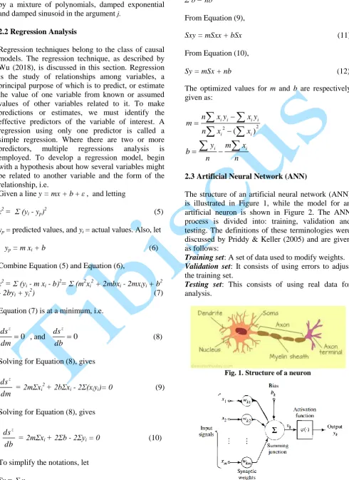
The structure of an artificial neural network (ANN) is illustrated in Figure 1, while the model for an artificial neuron is shown in Figure 2. The ANN process is divided into: training, validation and testing. The definitions of these terminologies were discussed by Priddy & Keller (2005) and are given as follows:
Training set: A set of data used to modify weights. Validation set: It consists of using errors to adjust the training set.
Testing set: This consists of using real data for analysis.
Fig. 1. Structure of a neuron
The model illustrated in Figure 2 is given in Equation (13) and Equation (14).
1 m
k j j
j
u w x
(13)and
k k k
y
u b (14)where x x1, 2,...,xm are the input signals;
1, 2,..., m
w w w are weights; ukis output; bk is the bias;
. is the activation function and yk is signal for ANN. Also,k k k
v u b (15)
where vk is activated by k. The linear combiner uk is modified bybk (Figure 3).
Fig. 3. ANN output
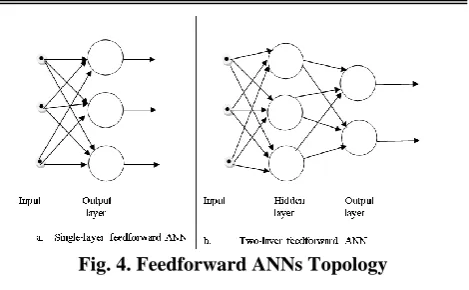
Artificial neural networks can be classified into: (i) Feedforward ANN
(ii) Feedback/Recurrent ANN i. Feedforward ANN
The topology of the Feedforward ANN is given by Figure 4.
ii. Feedback/Recurrent ANN
The Feedback/Recurrent ANN is based on results of previous processing inputs.
Fig. 4. Feedforward ANNs Topology
3. COMPARATIVE ANALYSIS OF THE TECHNIQUES
The inherent features of applying the machine learning techniques are summarized in Table 1. The techniques discussed in this section were examined to determine their strengths and weaknesses. The techniques summarized in this table include Box-Jenkins technique, regression analysis, and the artificial neural network (ANN). As a result, challenges in applying these techniques discussed and analyzed.
Table 1. Characteristics of machine learning techniques
Tech-nique
Positive Attributes
Negative Attributes
B
o
x
-J
enkin
s
1) Adapts multiple variables
2) Solution based on multi-variables 3) Simple input data. 4) Possible to adjust model to more variables 5) Discusses trends
1) Does not differentiate between components of variables
2) No explicit description of
components of variables 3) Need to identify a more appropriate technique for modeling 4) Does not specify requirements for individual variables 5) No information of specific effect of individual variables on dependent variable
Reg
re
ss
io
n Ana
ly
si
s
1) Incorporates multiple variables
2) Information on effect of individual variables on dependent variable 3) General mathematical model to estimate variables
4) Handles larger data than Box-Jenkins technique
5) Model shows when variables are included or not
1) Small and large transitions in time are under-represented in the model
Art
if
icia
l N
eura
l
Net
wo
rks
1) Discusses the use of multiple variables 2) Introduces artificial intelligence for model 3) Discusses modelling by validating and testing data.
4) Determines model’s behaviour.
(5) Handles large data
1) Does not specify model requirements for individual variables 2) No information of effect of individual variables on dependent variable.
4. CONCLUSIONS
An in-depth study of commonly used machine learning techniques has been carried out. Each technique has its own limitations and challenges. Modeling data requires a high degree of accuracy such that any deviation from expectation may result in obtaining accurate estimates. The techniques used in the various studies were existing machine learning techniques applied to heterogeneous problems. Based on the reviewed papers, the following challenges were identified for Box-Jenkins, regression analysis, and artificial neural networks (ANN):
1. The need to identify a more accurate and generic technique for predicting data.
2. The need for models to handle big data.
3. Lack of insight into the estimation of components for variables.
4. There is a need to apply a technique for modeling. 5. The study of the extent to which various components affect variables.
The artificial neural network (ANN) has being able to overcome all the challenges present for Box-Jenkins technique and regression analysis. The ANN technique is more reliable for predicting data compared with Box-Jenkins technique and regression analysis. The ANN technique will also help identify the contribution of components for the various variables that are considered in a study. The application of machine learning techniques to model data are related to model behavior and their interventions in various fields of study, including information technology. This research reveals similarities and differences, such as the characteristics of machine learning techniques. These reviewed studies have added to our understanding of how to model data using the techniques mentioned in this study.
REFERENCES
[Kal00] S. Kalogirou - Applications of artificial neural-networks for energy systems, Applied energy, vol. 67: 17-35, 2000.
[KS10] B. Kramer, J. Satzger - Power prediction in smart grids with evolutionary local kernel regression, Hybrid artificial intelligent systems, vol. 1(1): 262-269, 2010.
[N+02] F. J. Nogales, J. Contreras, A. J. Conejo, E. Espinola - Forecasting next-day electricity prices by time series models. IEEE Transactions on Power Systems, vol. 17(1): 342–348, 2002.
[Pat96] D. Patterson - Artificial neural networks. Singapore: Prentice Hall,
1996.
[PK05] K. Priddy, P. Keller - Artificial neural network - An introduction, USA SPIE international society for optical engineering, 2005.
[R+10] A. Ruzzelli, C. Nicolas, C. Schoofs, G. O’Hare - Real-time recognition and profiling of appliances through a single electricity sensor, 7th Annual IEEE Communications Society Conference on Sensor, Mesh and Ad Hoc Communication and Networks, 2010.
[Wu18] C. Wu - Regression Technique, Retrieved from
http://www.historyofinformation.com/e xpanded.php?id=2706, 2018.
[Y+00] S. Yao, Y. Song, L. Zhang, X. Cheng - Wavelet transform and neural networks for short-term electrical load forecasting. Energy conversion and management, vol. 41(18): 1975–1988, 2000.