www.atmos-meas-tech.net/8/2491/2015/ doi:10.5194/amt-8-2491-2015
© Author(s) 2015. CC Attribution 3.0 License.
Reconstruction of cloud geometry using a scanning cloud radar
F. Ewald, C. Winkler, and T. Zinner
Meteorologisches Institut, Ludwig-Maximilians-Universität München, Theresienstr. 37, 80333 Munich, Germany Correspondence to: T. Zinner ([email protected])
Received: 28 August 2014 – Revised: 10 May 2015 – Accepted: 28 May 2015 – Published: 19 June 2015
Abstract. Clouds are one of the main reasons of uncertain-ties in the forecasts of weather and climate. In part, this is due to limitations of remote sensing of cloud microphysics. Present approaches often use passive spectral measurements for the remote sensing of cloud microphysical parameters. Large uncertainties are introduced by three-dimensional (3-D) radiative transfer effects and cloud inhomogeneities. Such effects are largely caused by unknown orientation of cloud sides or by shadowed areas on the cloud. Passive ground-based remote sensing of cloud properties at high spatial res-olution could be crucially improved with this kind of addi-tional knowledge of cloud geometry. To this end, a method for the accurate reconstruction of 3-D cloud geometry from cloud radar measurements is developed in this work. Us-ing a radar simulator and simulated passive measurements of model clouds based on a large eddy simulation (LES), the ef-fects of different radar scan resolutions and varying interpo-lation methods are evaluated. In reality, a trade-off between scan resolution and scan duration has to be found as clouds change quickly. A reasonable choice is a scan resolution of 1 to 2◦. The most suitable interpolation procedure identified is the barycentric interpolation method. The 3-D reconstruc-tion method is demonstrated using radar scans of convective cloud cases with the Munich miraMACS, a 35 GHz scan-ning cloud radar. As a successful proof of concept, cam-era imagery collected at the radar location is reproduced for the observed cloud cases via 3-D volume reconstruction and 3-D radiative transfer simulation. Data sets provided by the presented reconstruction method will aid passive spectral ground-based measurements of cloud sides to retrieve micro-physical parameters.
1 Introduction
Clouds play an essential role in Earth’s climate due to their impact on Earth’s radiation budget. Still they are one of the greatest sources of uncertainty in future projections of climate (Houghton et al., 2001). Most radiative processes connected to clouds are extremely sensitive to cloud micro-physics and their temporal evolution. In particular, the re-lationship between aerosol and cloud microphysics remains in the focus of current research (Rosenfeld and Feindgold, 2003; Kaufman et al., 2005; Koren et al., 2005). The pro-cess of aerosol activation and the subsequent growth of cloud droplets define the vertical structure of cloud microphysics as discussed by Rosenfeld et al. (2008).
Measurements of these processes are either direct but lim-ited to small samples, i.e. in situ measurements from aircraft, or they are indirect, i.e. from active or passive remote sens-ing. Remote sensing techniques are in themselves limited to spatial and temporal snapshots of the microphysical pro-cesses within a cloud – but their advantage is their almost instantaneous acquisition of multidimensional data sets. For instance, an active cloud radar is well-suited to derive cloud macrophysics (e.g. their three-dimensional (3-D) geometry), but for the most part insensitive to small cloud droplets, and therefore only provides limited information on cloud parti-cle formation (Hobbs et al., 1985; Miller et al., 1998). On the other hand, passive solar techniques can derive cloud particle characteristics very well (Nakajima and King, 1990; Twomey and Cocks, 1989).
pro-files of cloud microphysics from cloud sides observed from a ground, air or space perspective. Although passive remote sensing has been very successful when applied to satellite data (e.g. from the Moderate-resolution Imaging Spectrom-eter (MODIS), Platnick et al. (2003)), it reaches its limits when applied to highly structured cloud fields at high spatial resolution. And it is just this type of challenge the proposed remote sensing of cloud sides is confronted with.
One of the biggest problems remains the illumination and shadowing of cloud surfaces due to their different exposi-tion to the sun. Effective radius retrievals like Nakajima and King (1990) are based on observations of spectrally differ-ent absorption of cloud droplets of differdiffer-ent sizes. Illumina-tion, shadowing, leakage and channelling of photons into ad-jacent cloud columns also have an influence on spectral ab-sorption in 3-D clouds (Davies, 1978; Davis et al., 1979; Var-nai and Marshak, 2002). Therefore, passive retrievals can be improved decisively, if these geometric effects can be com-pensated for.
In their studies, Varnai and Marshak (2002) and Marshak et al. (2006) systematically quantified the impact of 3-D diative effects on the retrieval of cloud droplet effective ra-dius. Both pointed out that heterogeneity effects by shadow-ing and illumination at a spatial resolution of 1 km do not get cancelled out when averaged over a 50 km2region. Locally, Vant-Hull et al. (2007) even found differences up to 5 µm be-tween illuminated and shadowed cloud parts.
In this work, we try to answer the question whether scan-ning cloud radar measurements can be used to reconstruct the cloud volume which could help passive microphysical re-trievals with these geometric effects. However, there seems to be no universal approach to quantify the accuracy of a volu-metric reconstruction in literature. In our work we are inter-ested in a correct high-resolution reconstruction of the cloud side facing the radar location to improve the retrieval of cloud microphysics using reflected solar radiation. In any case, the metric should focus on the application and on the used prop-erty of the reconstructed cloud field.
In recent studies, Fielding et al. (2013, 2014) have worked out ways to retrieve the 3-D field of LWC (liquid water con-tent) to address the problem of 3-D clouds in radiation clo-sure meaclo-surements at the surface. To this end they conducted numerical studies to find suitable scan strategies for a suc-cessful reconstruction of the 3-D LWC field. In their work they also investigated the influence of cloud radar sensitivity on modelled surface radiation fluxes. In order to investigate the impacts of imperfect microphysical retrievals, they used power-law relationships between radar reflectivity, LWC and cloud effective radius (Martin et al., 1994; Liu and Hallet, 1997).
This study will complement the previous work of Fielding et al. (2013) in its aim to analyse the impact of scan res-olution and interpolation methods on the reconstruction of a LWC field for one specific cloud. It differs from the approach of Fielding et al. (2014) in that LWC and the effective
ra-dius are not completely reconstructed on the basis of cloud radar measurements alone. Rather, this study tries to provide a cloud volume which could complement subsequent passive retrievals using radiance measurements from cloud sides.
In an effort to set up ground-based remote sensing of cloud sides, the 3-D cloud reconstruction technique presented will provide valuable additional information for passive retrievals from this perspective. For this task, the centre of considera-tion is put on the reconstrucconsidera-tion of cloud surfaces oriented towards passive sensors. Not only this specific application, but basically every remote sensing technique, especially pas-sive, can benefit from such a reconstruction of cloud sides.
In this study, we therefore want to address the following questions:
1. How do scan resolution and scan strategy impact the reconstruction of a single cloud?
2. Which interpolation method is best suited for this re-construction?
3. How does cloud radar sensitivity influence the perfor-mance of this task?
4. How feasible is this approach for real-world applica-tions?
The paper is organized as follows: Sect. 2 first introduces the theoretical toolbox used in the selection and development of the final reconstruction method. It is based on the combina-tion of data from a high-resolucombina-tion cloud model, a simple radar simulator and simulations of cloud side images from the reconstructed cloud fields. Next, the actual development of the reconstruction method is described in Sect. 3 including the choice of scan strategies, the data remapping and interpo-lation and the correction for mean cloud motion. In Sect. 4, this approach is subsequently applied to real-world cases. Fi-nally, conclusions are drawn and the limitations posed by real-world cases due to cloud radar sensitivity are discussed.
2 Experiment setup
2.1 LES model test bed and radar simulator
0 1 2 3 4 5 6 7
y
rang
e
[km]
LWP
0 1 2 3
height [km] LWC (x = 3.75 km)
0 1 2 3 4 5 6 7
x range [km] 0
1 2 3
he
igh
t
[km]
0.1 1 10 100 1000
0.1 0.5 1 1.5 2
LWC [g m-3][g mLWP-2]
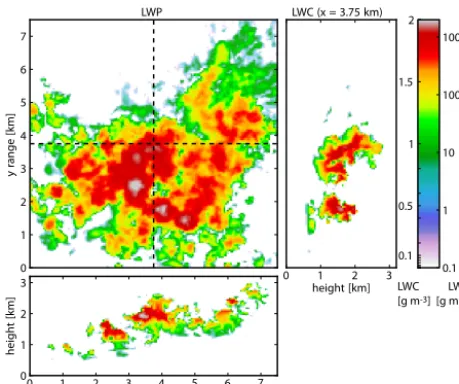
Figure 1. This figure shows the 7.5 km×7.5 km sub-domain of a trade wind cumuli large eddy simulation (Seifert and Heus, 2013) that was used to test the radar reconstruction under controlled con-ditions. The radar simulator was positioned in the lower left corner. The main figure shows liquid water path (LWP) in gm−2while the smaller figures on its bottom and to the right shows cross sections of LWC in g m−3forX= 3.75 andY = 3.75.
These data are well-suited for the evaluation of cloud geome-try reconstruction methods, because of their high spatial res-olution of (25 m) in all three dimensions over a domain that spans 50 km×50 km×4 km. For the radar scan simulations, only a smaller 7.5 km×7.5 km×4 km part of the domain is selected, as illustrated in Fig. 1. Throughout this study the radar is positioned in the lower left corner of the model do-main shown in Fig. 1. The UCLA-LES cloud model provides liquid water mixing ratios which can be translated to a radar reflectivity factor zfor each cloud box if a certain droplet radiusr0is assumed.
Considering the radar reflectivity factor z in units of mm6m−3,
z=26
∞ Z
0
N (r)r6dr. (1)
With a constant droplet radiusr0, this simplifies to
z=26N r06, (2)
whereN stands for the number of particles per volume. Be-cause values ofzcan span many orders of magnitude, they are normally expressed in form of the logarithmic radar re-flectivityZin units of dBZ:
Z=10 log10 z 1 mm6m−3
. (3)
The simulation of a radar scan is obtained from a single LES time step (att=32 h simulation time) i.e. not only a frozen
turbulence assumption is applied but the cloud motion is also neglected during the radar scan.
Radar reflectivitiesZ are determined along a number of beams in radial distances from the radar with a cloud radar range gate length of 60 m. The scan pattern is determined by specifying a number of consecutive beam directions in terms of elevation and azimuth angles (2and8). This way, mea-surement points in spherical coordinates are obtained. A ray tracer finds the LES grid box that contains each of the points. The radar reflectivity Z of this grid box is returned as the simulated measurement value.
Additionally, an option to simulate finite radar sensitivity is included. If turned off, everyZ value is accepted. Alter-natively a threshold is used to setz=0 for measurements smaller than a threshold. The distance-dependent threshold
Zminis set according to the minimal detectable radar reflec-tivity following Doviak and Zrnic (1993) and Riddle et al. (2012):
Zmin(d)=C0+10 log
τ0P
t0
τ Pt
+20 log
d+doffset
d0
+SNRmin[dB], (4)
SNRmin= Q
NFFTpKavg. (5)
Here,C0= −20.7 dB denotes the specific radar constant in logarithmic units for a reference distance of d0=5 km, a pulse duration ofτ0=200 ns, an average transmitter power ofPt0 =30W and includes a 2 dB finite receiver bandwidth
loss. The distance offsetdoffsetis used to shift the radar away
from the cloud without a change of geometry. This way, sen-sitivity can be analysed isolated from other changes due to the new measurement position. SNRmin is the minimal
de-tectable signal–noise ratio, which depends on the specific signal characteristics and its detection. During the scanning mode we incoherently averagedKavg=10 Doppler spectra
(totalling 0.5 s) obtained from the fast Fourier transforma-tion (FFT;NFFT=256) of backscattered radar signals, with a pulse length ofτ =400 ns and an average transmitter power ofPt=52W. In order to separate signal and noise floor, the
method described by Hildebrand and Sekhon (1974) with a threshold Q=5 was used. With this method a minimal SNRminof about−22.1 dB can be reached if the signal power
is contained within one FFT bin (Riddle et al., 2012). Using Eqs. (2)–(5) synthetic radar data are generated for a given cloud structure. In order to evaluate the quality of reconstruction possibilities for this structure, a measure of success is needed.
supporting passive microphysical retrievals from cloud sides, simulated radiances from cloud sides in the solar spectral range are the most meaningful quality measure for our pur-pose.
To this end, a “photo” of the reconstructed cloud is simu-lated. The radiative transfer model MYSTIC is used, a Monte Carlo code for the physically correct tracing of photons in cloudy 3-D atmospheres (Mayer et al., 1998; Mayer, 2009). MYSTIC is part of the radiative transfer library libRadtran (Mayer and Kylling, 2005). For an arbitrarily given cloud field, the corresponding observable radiance field can be de-rived with the MYSTIC panorama option (Mayer, 2009) if the viewing position and field of view are defined. The ra-diative transfer calculations are done at two wavelengths (870 nm and 2100 nm) which are used by the microphysical retrieval, proposed by Nakajima and King (1990). Since ra-diative smoothing is reduced considerably at 2100 nm, cloud morphology becomes more apparent due to reduced photon transport through clouds by enhanced liquid water absorption (Oreopoulos et al., 2000). For this reason, spectral radiance fields atλ=2100 nm are shown in Sect. 3.4 as greyscale im-ages of the cloud as it would be seen from the position of the cloud radar. By means of these images, reconstructed clouds can be compared to the original clouds from the LES or with a real camera image to discuss the performance of the recon-struction.
For these radiative transfer simulations, radar reflectivity factorsz, simulated or measured, have to be converted back into cloud microphysical properties. As we are more con-cerned about geometry than about reproduction of exact mi-crophysical properties, this step is simplified. As long as the microphysical properties are held constant the performance of different reconstruction approaches at 2100 nm can be analysed independently without relying on microphysical ap-proximations. For this reason, a fixed cloud droplet radiusr0
is assumed throughout the original cloud as well as the recon-structed cloud. Thus the number concentrationN in Eq. (2) can be replaced by the LWC which then leads to
LWC(z)=z·π·ρH2O
48·r03 . (6)
HereρH2Ois the density of water. For real measurements this
approach involves some difficulties: drizzle and/or rain with high reflectivities within a cloud lead to unrealistic high val-ues of LWC under the assumption of a fixed monodisperse cloud droplet sizer0. As high LWC – and therefore high op-tical thickness – leads to an extremely large number of scat-tering events simulated by the Monte Carlo model, compu-tational effort for the radiance simulation grows rapidly in these cases. Since this work is focused on the reconstruc-tion of cloud geometry, quantitative values of microphysical fields are not crucial as long as the cloud objects are opti-cally thick. Thus, a simple LWC cut-off at high values can be applied, equivalent to a certain maximum limit inz. The LWC field obtained this way is then the basis of 3-D
simula-Table 1. Technical specifications and operational parameters of the miraMACS cloud radar. If two values are given, the first one is used in vertical viewing mode, the one labelled with an asterisk is used in scan mode. PRF is the pulse repetition frequency andNFFTis the number of consecutive pulses used for one Doppler spectrum.
Parameter Value
Model METEK MIRA-35S
Frequency 35 GHz
Wavelength 8.4 mm
Beam width 0.6◦×0.6◦
Peak power 30 kW
PRF 5 kHz
NFFT 256
Incoherent averages 200, 10∗
Vertical resolution 30, 60∗m
Sensitivity (best case) in 5 km −48.8,−48.3∗dBZ
tions, providing radiance images to compare reconstruction and original cloud geometry.
This comparison can be conducted by the human eye, quite a powerful instrument in detecting reconstruction problems. A more objective way of comparison is the root mean square error (RMSE) of the difference between simulated radiance fields of reconstructed and original cloud fields. In order to make this comparison independent from cloud microphysics, the radiative transfer simulation for the original LES cloud field was done with the same fixed cloud droplet radiusr0. 2.3 The miraMACS cloud radar
Real radar measurements discussed here are obtained with the miraMACS cloud radar – a scanning ground-based 35 GHz, 8.4 mm wavelength MIRA35-S cloud radar, man-ufactured by METEK GmbH. It is located on the roof of the Meteorological Institute Munich as part of the Munich Aerosol Cloud Scanner project (MACS). It features full hemispheric scanning with a scan speed of up to 10◦s−1. In Table 1, an overview of specifications of the miraMACS radar system is given. For the reconstruction of cloud ge-ometry, the effective radar reflectivity factors provided by the METEK data processing software were used (Bauer-Pfundstein and Görsdorf, 2007).
3 Development of reconstruction procedure
Cloud Cloudradar resolutionscan
Interpolation interpolationmethods
Gridded LWC
3D RTM
Image Image
camera
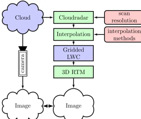
Figure 2. Illustration of the process chain leading from a radar scan to the 3-D cloud reconstruction. Influence of scan resolution and interpolation method is analysed by the comparison of the simulated cloud field and the camera picture of the original cloud.
distributed measurements to a regular grid. This step con-cludes the reconstruction itself. This step is followed by the quality test (see Sect. 2.2), which consists of the comparison of a synthetic radiance image from the LES data, or a real camera picture recorded during the scan and radiance sim-ulations based on the reconstructed cloud volume. The in-dividual steps and reconstruction parameters and methods analysed during testing are presented in more detail in the following.
3.1 Scan strategies
Scan pattern and scan resolution are among the first param-eters to be chosen. In their study Fielding et al. (2013) con-ducted extensive research on the potential ability of differ-ent scan strategies to reconstruct 3-D clouds. Their work proved that a scan mode perpendicular to the wind direction at a fixed azimuth yields the best results for radiation closure studies, with an advection wind speed above 10 ms−1. More-over, they argue that sector-type scan modes are not the best choice for radiation closure. Since we are searching for ad-ditional information on radiance measurements from cloud sides, sector-type scan modes are our tool of choice. These scan strategies allow simultaneous measurements of specific cloud sides with collocated solar radiance measurements. In addition, the higher spatial sampling density of facing cloud sides is another decisive argument for this kind of scan strat-egy.
Two of these sector-type scan modes are the sector range– height indicator (S-RHI) scan pattern, which is a vertical el-evation scan for a stepwise-changing azimuth angle, and the sector plane–parallel (S-PPI) scan pattern which is a
hori-Figure 3. Visualization of the simulated S-RHI scan pattern within the cloud model domain. The cloud radar is positioned in the lower left corner (red point). For illustrative purposes only, selected slices of the 45 scans of a 90◦azimuth range S-RHI scan with a 2◦ reso-lution are shown.
zontal azimuth scan for stepwise changing elevation angle. Figure 3 shows the overall geometry of the S-RHI pattern used in this study. The figure shows four representative ele-vation scans for the used LES cloud field. The cloud radar is situated at the lower left corner marked with the red point in Fig. 3. In our study S-RHI is favoured over S-PPI, be-cause it can be used to partially correct for the cloud motion component tangential to the radar position. A wind profile from a nearby radiosonde station can then be used to com-pensate for the horizontal drift of the cloud. In this way, the S-RHI produces consecutive vertical profiles which better fit subsequent retrievals of vertical profiles of cloud micro-physics. Moreover, the S-RHI scan reconstruction only gets compressed or stretched by deviations of the local cloud drift from the mean wind profile. The vertical structure of the S-PPI reconstruction would get torn apart from the mean wind profile by deviations. For these reasons the S-RHI scan pat-tern seems to be the better choice for the reconstruction of isolated cloud sides.
instru-ment. Since Fielding et al. (2013) found that surface irradi-ance RMSE during a 5 min scan period can already be sub-stantial, we limited the time duration of scan patterns to 5 min to minimize the errors associated with the temporal evolution of the cloud that are caused by turbulence and convection during the acquisition.
The specific trade-off between scan resolution and scan duration depends on the distance of the cloud (the larger the distance, the higher the angular resolution has to be) and the settings that determine the time to measure one profile (pulse repetition frequency, spectral averaging of spectra). In addi-tion, the evolution timescale and motion speed of a specific cloud has to be taken into account (turbulent convective vs. more static). For a cloud 5 km away, the anticipated horizon-tal resolution of the front-facing cloud side lies between 100 and 200 m. In view of these constraints, the scan resolution of the current cloud radars hardly reach the high spatial resolu-tion of current passive imaging radiometer. Nevertheless, this spatial resolution still gives additional information for clouds with a cloud base of 2–5 km. Choices of scan speed and scan resolution will be shown in Sect. 4 for specific applications on miraMACS data.
A compromise must be found between a dense azimuthal sampling, noise reduction by temporal averaging and the du-ration to scan a complete cloud scene, in order to optimize the approximation of the volumetric reconstruction. Addi-tionally, one has to consider that most current cloud radar systems have to rotate their antenna to acquire multidimen-sional scans. In the case of the miraMACS cloud radar, the scan speed is limited to 10◦s−1by the inertia of its scanner. It became evident in miraMACS measurements of stratiform, and therefore stationary cloud profiles, that a temporal av-eraging overtavg = 0.5 s for one profile almost reached the maximum sensitivity obtained withtavg =10 s. The
combi-nation of a temporal averaging over t = 0.5 s with an an-gular scan velocity of 4◦s−1has subsequently proven to be a feasible compromise between noise reduction and spatial sampling density. Consecutive beam profiles with an angular opening of 0.5◦are then acquired with a vertical resolution of 2◦. It therefore takes roughly 5 min to complete a S-RHI scan of 45◦in azimuth and 50◦in elevation with an azimuthal resolution of 2◦.
3.2 Remapping radar data to Cartesian space considering cloud motion
The measured data points are stored in spherical coordinates, the distance (d) from the radar, together with the elevation angle (2) and the azimuth angle (8) of the beam. They are then remapped to Cartesian coordinates(x, y, z).
The time period for a 90◦azimuth range S-RHI scan with adequate resolution and scan speed is in the order of min-utes. Depending on the atmospheric conditions, the cloud can change its position and its shape significantly during this pe-riod. A complete consideration of this 3-D motion
includ-ing turbulence is not achievable with current cloud radar sys-tems.
Nonetheless, the main horizontal wind direction tangential to the radar position can be corrected. To this end the wind profile from a nearby atmospheric sounding can be used. Let
t0be the central time of a scan period. Each radar
measure-ment has a timetiand a location(x(ti), y(ti), z(ti)).
Accord-ing to the wind speedu inx direction andv iny direction taken from a radiosonde profile,x(ti)andy(ti)are shifted
to their approximate position at timet0(usingz(ti)to select
best vertical level in the sounding):
x(t0)≈x(ti)+u·(t0−ti) (7)
y(t0)≈y(ti)+v·(t0−ti). (8)
Thus, early measurements are shifted downwind; later mea-surements are shifted upwind.
The subsequent interpolation was done on the full do-main size of 7.5×7.5×4 km with a coarser grid spacing of 50×50×25 m for computational efficiency. Since we fixed the effective radiusreffthroughout the domain, the
con-version from radar reflectivity zto LWC (Eq. 6) produced equivalent results whether we applied it before or after the linear interpolation. When cloud effective radius is directly connected to LWC using e.g. a power-law relationship like Fielding et al. (2013), the conversion with Eq. (6) should happen before the interpolation. This happens as the linear relationship between radar reflectivityzand LWC in Eq. (6) becomes non-linear when inserting Eq. (1) with a variable cloud effective radius.
3.3 Interpolation methods
The interpolation of the scattered radar data on a dense reg-ular grid is the central reconstruction step. The reconstructed LWC field is necessary for all subsequent steps (radiance simulation, 3-D display of the cloud, application in passive cloud side remote sensing).
The sparse and inhomogeneously distributed data make the interpolation challenging. In addition, the sensitivity limit with respect to small cloud droplets leads to some uncertainty in the definition of cloud boundaries. In order to consider these challenges, several interpolation methods and param-eters were tested in the controlled environment of the LES cloud case: nearest-neighbour interpolation (NNE), inverse distance weighting (IDW) (Shepard, 1968), barycentric terpolation (BAR) (Möbius, 1976) and natural neighbour in-terpolation (NAT) (Sibson, 1981).
singu-Figure 4. Illustration of the underlying concepts of barycentric and natural neighbour interpolations. (left) The barycentric method is based on the Delaunay triangulation (grey lines) for a point set of measurement points (all coloured points, except the red one). If the measurements are going to be interpolated at the position of the red point, the coloured triangle formed by the yellow, magenta and cyan points has to be considered. The values at these points are then weighted corresponding to the area of their opposite, same-coloured sub-triangle to interpolate the field at the red point. (right) Natural neighbour interpolation is based on the Voronoi tessellation. The Voronoi cell for a single measurement point is defined by all median lines (black) between the point and all vertices of triangles the same point belongs to. The overlap between former Voronoi cells and the Voronoi cell of the interpolation point (red) determines its natural neighbours and defines the weighting of their values.
lar red point, where the measured field is unknown and is subsequently interpolated. Figure 4 shows the Delaunay tri-angulation for a set of exemplary measurements on the left. The Delaunay triangulation maximizes the minimum angle within all triangles in the triangulation in such a way that no point lies inside any circumcircle of all the triangles (Delau-nay, 1934). In this way the three vertices of a triangle are the three nearest points for each point within the triangle. This triangulation is directly related to the Voronoi tessellation as its dual graph which is shown on the right in Fig. 4. The Voronoi cell for a single point is defined by all median lines between this point and vertices of triangles the same point belongs to. In this way the Voronoi cell marks the nearest-neighbour region for this point.
3.3.2 Nearest-neighbour interpolation
The properties of the Voronoi tessellation relate directly to the nearest-neighbour method. It is the simplest interpolation method and is based on the Euclidean distanced(x, xj)
be-tween pointsxandxj. The value of a functionF for a given
pointx is simply the valuefj for the nearest pointxj that
minimizes the Euclidean distanced(x, xj):
F (x)=fj for some xj with d(x, xj)=min
j d(x, xj). (9)
This method neglects the values of all other neighbouring points. The interpolated field therefore exhibits jump discon-tinuities and rough edges.
3.3.3 Shepard’s method
One interpolation method that overcomes this problem is the Shepard method (Shepard, 1968) also known as inverse distance weighting. Here, the value of a function F for a given pointx is a weighted average of all known valuesfj
at the known pointsxj. The known valuesfj are averaged
with their weightwj, the inverse of the Euclidean distance
d(x, xj)to the power of the parameterp:
wj(x)=
1
d(x, xj)p
. (10)
The valueF (x)is then the averaged sum of all known fj
withwj:
F (x)=
PN
j=0wj(x)fj
PN
j=0wj(x)
, ifd(x, xj)≤dmaxfor allj
fj, ifd(x, xj)=0 for some j
. (11)
Due to the inverse of the distance, the weightswj decrease
for points far away from x. The power parameterp deter-mines how fast these weights decrease. For points inRk the
power parameter has to bep > k because otherwise F (x)
would be dominated by points far away instead of points nearby. Since the cloud radar measurements are distributed 3-dimensionally in space, for S-RHI scan patterns the power parameterp =4 is chosen.
For p→ ∞ this method converges towards the result of a nearest-neighbour interpolation. One advantage of this method is the smoothness of the interpolated field. The dis-advantages are its high computation cost as the number of points increase and the so-called bull’s-eye effect which cre-ates circular regions around data points due to the rapidly growing weightwj.
3.3.4 Barycentric interpolation
This interpolation method is based on the barycentric coordi-nate system. InR2, these coordinates are also known as areal
coordinates. They are proportional to the areas of the three triangles that are formed by joining pointx (red point) with each vertexxj (yellow, magenta, cyan) of the triangle1R,
enclosing pointx (see Fig. 4, left). For1Rall values of the barycentric coordinates for pointxare positive. As shown on the left in Fig. 4, the valueF (x)atxis a linear interpolation of the valuesfj at the known verticesxj of1R. The value fj at each vertexxj is thereby weighted by the area of the
opposing triangle. The weights are normalized with the total area of1R(see Fig 4).
Arithmetically, the barycentric method is a variant of La-grange polynomial interpolation; values ofF (x)are repre-sented as a linear combination of valuesfjand the Lagrange
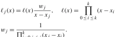
basis polynomials`j: F (x):=
k X
j=0
fj`j(x), `j(x):= Y
0≤m≤k
m6=j
x−xm xj−xm
For a given set of measurement points xj, the part wj in `j(x)is independent from pointxfor whichF (x)is
interpo-lated. With so-called barycentric weights wj, the Lagrange
basis polynomials can be written as
`j(x)=`(x)
wj
x−xj
, `(x)=
k
Y
0≤i≤k
(x−xi),
wj =
1 Qk
i=0,i6=j(xj−xi)
. (13)
The term `(x) can be eliminated by dividing (Eq. 12) by the interpolant of the constant functionF (x)=1. This then yields the second form of the barycentric formula:
F (x)=
Pk j=0
wj x−xjfj
Pk j=0
wj x−xj
. (14)
Based on Eq. (13) it becomes clear that the barycentric weightswj can be pre-computed for a given set of
measure-ment points xj which speeds up the subsequent
interpola-tion of F (x). Moreover, Berrut (1988) proved the conver-gence and numeric stability of barycentric interpolation for scattered as well as for equispaced points. In particular, the measurement pattern of a scanning cloud radar with its linear beams and its diverging scan curtains comprises scattered as well as equispaced measurement points. The produced fields are continuous and the interpolation adapts itself to the local measurement geometry.
3.3.5 Natural neighbour interpolation
Natural neighbour interpolation (Sibson, 1981) is based on the Voronoi tessellation of a given point set xj. Contrary
to barycentric interpolation, this interpolation includes not only the three vertices of the enclosing triangle for point
x, but all its natural neighbours. Natural neighbours can be understood by the adjacent Voronoi cells of point x when pointx is contained in the Voronoi tessellation of the given point set. The area of each former Voronoi cell that is lost to the newly formed Voronoi cell of pointx determines the interpolation weight wj for the valuefj atxj (see Fig. 4,
right). Natural neighbour interpolation produces continuous and smooth fields while it remains computationally complex (Park, 2006).
The next figure shows the Delaunay triangulation (Fig. 5, left) and the Voronoi tessellation (Fig. 5, right) of the pro-posed S-RHI scan pattern for one elevation height. For both methods with increasing radial distance, the grid cells adapt naturally to the increasing lateral distance between adjacent scans. All methods discussed are not limited toR2but can be generalized to Rk. In the case of cloud radar measure-ments (R3), the Delaunay triangulation is based on tetrahe-drons while the Voronoi tessellation is based on convex poly-hedrons.
Figure 5. For one scan elevation both panels show qualitative cross sections of the measurement locations (blue) and the underlying in-terpolation meshes (green) for the 90◦azimuth range S-RHI scan shown in Fig. 3. Throughout this plots the cloud radar is located in the lower left corner. (left) This panel gives an idea of the overall structure of the Delaunay triangulation, which is the basis of the barycentric method. The more acute-angled triangles at greater ra-dial distances can produce artefacts as discussed in Sect. 3.4. (right) Here, the corresponding exemplary Voronoi tessellation of the S-RHI scan pattern (Fig. 3) for one scan elevation is shown. The sin-gle Voronoi cells adapt naturally to the increasing lateral distance between adjacent scans.
3.4 Analysis of scan resolution and interpolation effects
Figure 6a shows an example radiance image as it would be seen from the position of the cloud radar at the lower left in the LES data. Each pixel is related to a pair of azimuth and elevation angles[8, 2]between 0 and 90◦ and 0 and 70◦i.e. the image is comparable to a wide-angle photo. In Fig. 6 the cloud side of the main cloud element is visible, illuminated from a sun zenith angle of 60◦ directly in the back of the sensor. The central cloud element is about 6.5 km wide and 3 km high (cf. Fig. 1). Apparently, additional clouds become visible towards the horizon due to periodic boundary conditions of the radiative transfer simulation.
Figure 6b–f show the results for the tests of different radar scan resolutions for the cloud situation shown in Fig. 1 when the barycentric method is used. In this figure comparisons of Monte Carlo radiance simulations at 2100 nm of cloud recon-structions are shown for different scan resolutions between 1 and 5◦. It can be seen in Fig. 6 that details of brightness gradients and the overall image contrast get washed out for coarser scan resolutions. The RMSE between interpolated and original clouds increases linearly from 0.69 (23.21) to 1.38 (34.75) mW m−2sr−1nm−1at 2100 nm (resp. 870 nm)
for scan resolutions from 1◦to 5◦. Simultaneously with the RMSE, the radiance bias for both wavelengths increases with coarser resolution. Detailed radiance results can be found in the right two columns of Table 2.
0 10 20 30 40 50
Θ
[
deg
]
(a) (b)
0 10 20 30 40 50
Θ
[
deg
]
(c) (d)
0 4 8 12 16 20 24 28 32 36 40 44 48 52 56 60 64 68 72 76 80 84 88
Φ[deg]
0 10 20 30 40 50
Θ
[
deg
]
(e)
0 5 10 15 20 25 30 35 40 45 50 55 60 65 70 75 80 85 90
Φ[deg]
(f)
0 2 4 6 8
L[mW m−2sr−1nm−1]
Figure 6. Comparison of reconstruction result for different scan resolutions. Panel (a) shows the true high-resolution radiance panorama at 2100 nm. Other panels show the radiance panorama for reconstructions at elevation and azimuth angle resolution of (b) 1◦, (c) 2◦, (d) 3◦, (e) 4◦and (f) 5◦. Interpolation method is barycentric (cf. Fig. 7).
of Fig. 7, some disadvantages of the different interpola-tion methods are already visible. A nearest-neighbour in-terpolation (Fig. 7a) produces box structures which become clearly visible when doing 3-D radiative transfer calcula-tions. Though smoother in appearance, the Shepard method (Fig. 7b) leads to circular artefacts at cloud edges. These cir-cular regions around data points are caused by the already mentioned bull’s-eye effect. The reason for this artefact and the problem it is causing for measurements on a variable grid spacing will become more clear in the following liquid water path (LWP) analysis.
Judging with the human eye, the deviation in radiance fields of the reconstructed cloud compared to the original model cloud seems lowest for barycentric (Fig. 7c) and nat-ural neighbour interpolations (Fig. 7d). However, the RMSE between the radiance fields of the reconstructed clouds and
the original cloud does not clearly show these differences. The values at 2100 nm range from 1.09 mW m−2sr−1nm−1 for Shepard to 0.87 mW m−2sr−1nm−1 for barycentric and natural neighbour interpolations (see Table 2).
be-0 10 20 30 40 50
Θ
[
deg
]
(a) (b)
0 10 20 30 40 50 60 70 80 90
Φ[deg]
0 10 20 30 40 50
Θ
[
deg
]
(c)
0 10 20 30 40 50 60 70 80 90
Φ[deg]
(d)
0 2 4 6 8
L[mW m−2sr−1nm−1]
Figure 7. Comparison of reconstruction results for different interpolation methods on the basis of the high-resolution radiance field at 2100 nm. Results are shown for (a) nearest-neighbour, (b) inverse distance weighting, (c) barycentric and (d) natural neighbour interpolations when applied to 2◦scan data.
Table 2. Quality measures for cloud reconstructions when using different scan resolutions and interpolation methods. Numbers after the method abbreviations indicate the scan resolution used, in degrees. The first columns show the liquid water path (LWP) bias of the recon-structed cloud field in g m−2and percentage. The latter two columns show the spectral radiance bias and its RMSE in mW m−2sr−1nm−1 of simulated cloud sides at 870 nm and 2100 nm (Figs. 6b–f, 7a–d) when compared to the original cloud (Fig. 6a). In each column the best performance is highlighted in bold.
LWP(g m−2) L∗870 L∗2100
Method Bias Percent Bias RMSE Bias RMSE
for 2-degree scan resolution
NNE2 +0.4 +0.5 % +7.87 27.89 +0.05 0.89
IDW2 +0.5 +0.7 % +8.58 30.58 +0.35 1.09
NAT2 +0.3 +0.4 % +8.97 25.78 +0.17 0.87
for 2–5-degree scan resolution
BAR2 +0.0 +0.0 % +7.63 27.07 +0.14 0.87
BAR3 +0.5 +0.7 % +9.95 28.51 +0.27 1.05
BAR4 −2.3 −3.0 % +8.29 32.89 +0.28 1.20
BAR5 +2.1 +2.7 % +10.60 34.75 +0.40 1.38
for 5-degree scan resolution
NNE5 +2.7 +3.5 % +9.27 34.21 +0.11 1.36
IDW5 +2.9 +3.8 % +10.15 36.84 +0.56 1.51
NAT5 +2.1 +2.8 % +8.72 37.16 +0.41 1.40
0 1 2 3 4 5 6 7 y rang e [km] LWP
0 1 2 3 height [km] LWC (x = 3.75 km)
0 1 2 3 4 5 6 7 x range [km]
0 1 2 3 he igh t [km] 0 1 2 3 4 5 6 7 y rang e [km] LWP
0 1 2 3 height [km] LWC (x = 3.75 km)
0 1 2 3 4 5 6 7 x range [km]
0 1 2 3 he igh t [km] 0.1 1 10 100 1000 0.1 0.5 1 1.5 2 0 1 2 3 4 5 6 7 y ra ng e [km] LWP
0 1 2 3 height [km] LWC (x = 3.75 km)
0 1 2 3 4 5 6 7 x range [km]
0 1 2 3 he igh t [km] 0 1 2 3 4 5 6 7 y ra ng e [km] LWP
0 1 2 3 height [km] LWC (x = 3.75 km)
0 1 2 3 4 5 6 7 x range [km]
0 1 2 3 he igh t [km] 0.1 1 10 100 1000 0.1 0.5 1 1.5 2 LWC [g m-3][g mLWP-2] LWC [g m-3][g mLWP-2]
(a) (b)
(d) (c)
Figure 8. Evaluation of cloud reconstructions generated with different interpolation techniques. Each main figure shows LWP in gm−2, while the smaller figures on its bottom and to the right shows cross sections of (LWC) in g m−3forX= 3.75 andY =3.75. The true cloud field is shown in Fig. 1. Panel (a) shows the result from nearest-neighbour, (b) inverse distance, (c) barycentric and (d) natural neighbour interpolations (cf. Fig. 7).
comes dominant at cloud edges. The circular artefacts seen in the radiance field (Fig. 7b) can be traced back to patterns in the horizontal LWC cross sections (shown in Fig. 8b). This artefact occurs at cloud edges around measurement points with low or zero values of LWC and is caused by the vicinity of points with large LWC values within the cloud.
With both methods the artefacts of the scan pattern re-main imprinted in LWP fields and LWC fields. In contrast, barycentric (Fig. 8c) and natural neighbour interpolations (Fig. 8d) yield much smoother results. Also, both methods produce very similar fields. The shape of the cloud bound-aries appears smooth in the LWP as well as the LWC field. Both interpolations result in a slightly blurry reconstruc-tion compared to the original cloud field, especially at cloud edges. Here, natural neighbour interpolation produces blur-rier fields of LWC and LWP compared to the barycentric approach. A distinct difference exists for regions far away
from the radar position. The LWP interpolated by the nat-ural neighbour method becomes too smooth compared to the original LWP field. This is due to decreasing measure-ment density as the radial distance increases. Contrary to this, the structure of the barycentric LWP field gets unnaturally stretched in the lateral direction. This happens because the tetrahedrons of the Delaunay triangulation get stretched in the lateral direction at larger radial distance, while the mea-surement density in the radial direction stays constant.
10−3 10−2 Frequency [Hz]
100 101 102 103 104 105
Spectr
al
Density
of
LWC
[g
2m
−
6]
Original Natural Neighbor Nearest Neighbor Barycentric Shepard
102 103
Spatial Scale [m]
Figure 9. Comparison of PSD of the reconstructed LWC fields (compare Fig. 7) for different interpolation methods and 2◦scan resolution. The black line shows the PSD for the true LWC field. The other lines show the PSD for the reconstructions using nearest-neighbour (blue), Shepard (yellow), barycentric (green) and natural neighbour (red) interpolations (cf. Fig. 7).
of around 3%, while barycentric interpolation performs best (2.7%).
A more comprehensive analysis of the different methods can be made when the LWC fields are compared in the fre-quency domain. In Fig. 9, the power spectral density (PSD) of the LWC fields is shown for the different reconstruction methods when given the radar data with a scan resolution of 2◦. Naturally, all reconstructed LWC fields fall short in repro-ducing the small-scale LWC fluctuations. While the nearest-neighbour method produces gradients that are too strong, the returned fields for all other interpolation methods are too smooth. This behaviour becomes dominant at scales be-low the spatial sampling frequency (which varies between 50 and 250 m as a function of the radial distance). The natural neighbour interpolation field becomes too smooth while the barycentric and Shepard methods reproduce the original PSD the best. Since the Shepard method did not perform as well as the other two methods in the reconstruction of the radi-ance field (Fig. 7) and also showed problematic artefacts in the synthetic LWC field (Fig. 8), it is not taken into consider-ation. The tendency of the natural neighbour method to pro-duce fields which are too smooth becomes more pronounced towards the 5◦ scan resolution. This is shown in Fig. 10 where the variation of the PSD between 1 and 5◦is plotted for the natural neighbour (red) and barycentric (green) meth-ods. It is evident that the PSD for barycentric interpolation is less affected by scan resolution compared to the PSD for natural neighbour interpolation.
The analysis showed that for radiance field reconstruc-tions, the choice of scan resolution clearly overrides the choice of interpolation method. This finding is reflected in Table 2 for RMSE in radiance and also holds true for
re-10−3 10−2
Frequency [Hz] 100
101 102 103 104 105
Spectr
al
Density
of
LWC
[g
2m
−
6]
Original Natural Neighbor Barycentric
102 103
Spatial Scale [m]
Figure 10. Comparison of the variability of the PSD of the recon-structed LWC fields (compare Fig. 7) with different scan resolu-tions. The black line shows the PSD for the true LWC field. The green shaded area encloses the PSDs of barycentric interpolation. The red shaded area encloses the PSDs of natural neighbour inter-polation. Thereby the dashed line represents the 5◦scan resolution, while the solid line represents the 1◦scan resolution (cf. Fig. 6).
constructed LWP fields. While the nearest-neighbour method performed surprisingly well in numbers, the inverse distance weighting method has limitations in its use for the recon-struction of cloud liquid water fields as well as radiance fields from cloud sides. As previous studies (Trapp and Doswell, 2000; Zhang et al., 2005) have already shown, the choice of weighting function is important for retaining the spatial re-flectivity structures. Since we are looking for a stable method that is adaptive to a variable 3-D data point spacing, the sim-ple inverse distance weighting method seems unsuitable for the simultaneous reconstruction of cloud sides and the over-all cloud liquid water field. Combined with the findings in the frequency domain and due to its superior numerical stability (Berrut and Trefethen, 2004; Higham, 2004), the barycentric method appears to be the most suitable interpolation method for our application. In subsequent applications the S-RHI scan strategy with a resolution of 1 to 2◦and a barycentric interpolation will be used to reconstruct the 3-D cloud ge-ometry.
3.5 Sensitivity to detection threshold
In cloud radar science there is always the question to which extent cloud boundaries measured by radar are equivalent to the ones found by optical means, e.g. by lidar or by the hu-man eye. This can be explained with the low sensitivity with respect to small droplets and to small droplet number concen-trations (see Eq. 2). This leads to microwave signals which are too small to be detected, even though the backscattered signal at shorter, optical wavelengths is well-measurable.
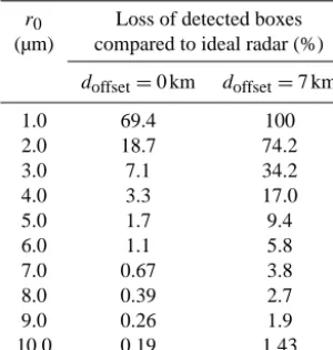
Table 3. Loss of detected cloud boxes due to radar detection thresh-old compared to an ideal radar in a simulated cloud (false nega-tives). Different values of droplet radii(r0)are assumed forZe cal-culation.doffsetdetermines the distance between radar and cloud side in the calculation of the detection threshold. In total, 12 155 cloud boxes could be detected by an ideal cloud radar.
r0 Loss of detected boxes
(µm) compared to ideal radar (%)
doffset=0 km doffset=7 km
1.0 69.4 100
2.0 18.7 74.2
3.0 7.1 34.2
4.0 3.3 17.0
5.0 1.7 9.4
6.0 1.1 5.8
7.0 0.67 3.8
8.0 0.39 2.7
9.0 0.26 1.9
10.0 0.19 1.43
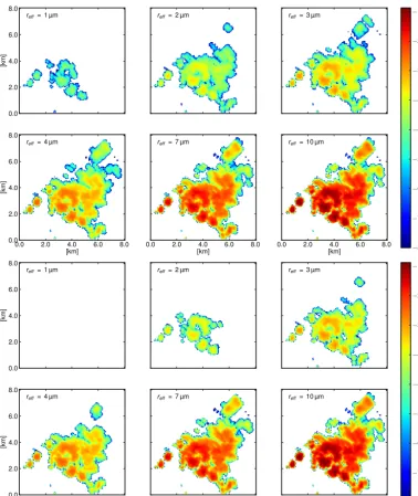
met. To this end, some further studies were conducted for the LES cloud data. As before, the radar simulator was situ-ated in the lower left corner, but this time with varying val-ues of droplet radius (r0) which affects the radar reflectivities (Eq. 2) and a varying distance between radar and cloud. All simulated radar scans were performed with 2◦resolution in elevation and azimuth angles. Interpolation is done with the barycentric neighbour method. In Fig. 11 results are shown for r0 ranging from 1 to 10 µm and for a distance between
radar and closest cloud side of about 3 (top) and 10 km (bot-tom). As one would expect from Eq. (2), the cloud is detected better the larger the droplets are and the closer the cloud is situated to the radar site. In our case this is reflected by the number of cloud boxes which lie above a particular detection threshold (see also Table 3). This number decreases with ris-ing sensitivity threshold. If a relative loss of 10 % of detected cloud boxes compared to a measurement with an ideal radar is defined as an acceptable limit, the required droplet radius is 3 µm (resp. 5 µm) for a distance of 3 km (resp. 10 km). These simplified values should provide a guideline for the assess-ment of the following real reconstruction cases. Several ad-ditional limitations affect the realistic estimation of detection thresholds in reality. The detection threshold as defined in Eq. (4) is therefore the only upper boundary of the sensitiv-ity a perfect radar would exhibit. Atmospheric absorption and broadening of the Doppler spectrum due to turbulence atten-uate the signal power received in each velocity bin inside the receiver.
4 Application of the cloud reconstruction method Reconstruction of convective clouds
So far, presented results and arguments are all based on syn-thetic data only. In the following, application of the recon-struction technique to real data will be shown. Two different cases illustrate possibilities and limitations. Both have been measured during the summer season of 2013 with the mira-MACS cloud radar on the roof of the Meteorological Institute in the centre of Munich.
The first demonstration case is based on a radar scan which was collected on 30 July 2013, 09:17–09:21 UTC. During the scan, a picture of the cloud was recorded by a camera, which is mounted on the radar and points in beam direction (Fig. 12, left). The scan covered an azimuth range of 20◦and an elevation range of 16◦. From left to right (i.e. north to south), 15 RHIs were scanned, leading to an azimuth resolu-tion of about 1.3◦. The scan speed was 1◦s−1which corre-sponds to a duration of about 4 min to scan the whole cloud. In combination with an averaging time of 0.5 s, this results in a 0.5◦resolution in the elevation direction. A simple esti-mation for the spatial resolution (1r) in dependence of the distanced to the radar and the resolution in degree 1α is given by1r=2·d·sin(1α). With the closest cloud side at a distance of about 13 km to the radar, this leads to a res-olution of about 300 m in azimuth and about 110 m in the elevation direction. The radial resolution (determined by the radar range gate length) is 60 m.
Applying the described method (Sect. 3), a field of regu-larly spaced (1x=1y=1z=100 m)zvalues was recon-structed. These radar reflectivity factors were converted to a field with values of LWC and droplet radius according to Sect. 2.2. This time the droplet radius was set constant to
r0=7.5 µm, the Ze-cut-off was chosen to be at −25 dBZ,
corresponding to a maximal LWC of 0.35 g m−3. A MYS-TIC 3-D simulation provides a colour image (by simulating red, green and blue channels, Fig. 12, right) with field-of-view and spatial resolution, matching the resolution of the installed camera. The images compare reasonably well (cf. Fig. 12, right).
The second case that is presented here is based on a scan on 25 July 2013 that took place between 15:23 and 15:27 UTC. This scan covered a range of 30◦ in azimuth and 28◦ in the elevation direction (see camera picture in Fig. 13, left) and took about 4 min to scan the cloud. With a scan speed of 2◦s−1and an averaging time of 0.5 s, a
res-olution of 1◦ was reached on the elevation axis. On the azimuth axis, a 1◦ resolution was also obtained. Since the wind speed was much higher on this day, the cloud mo-tion correcmo-tion was even more important. The distance of the cloud, between 17 and 27 km, was partly beyond the range of the radar. Interpolation was done at an equidistant 100 m grid, leading to a field ofZe values and related
0.0 2.0 4.0 6.0 8.0
[km]
reff= 1 µm reff= 2 µm reff= 3 µm
0.0 2.0 4.0 6.0 8.0
[km] 0.0
2.0 4.0 6.0 8.0
[km]
reff= 4 µm
0.0 2.0 4.0 6.0 8.0
[km]
reff= 7 µm
0.0 2.0 4.0 6.0 8.0
[km]
reff= 10 µm
−80
−72
−64
−56
−48
−40
−32
−24
−16
Ze
/
dB
Z
0.0 2.0 4.0 6.0 8.0
[km]
reff= 1 µm reff= 2 µm reff= 3 µm
0.0 2.0 4.0 6.0 8.0
[km] 0.0
2.0 4.0 6.0 8.0
[km]
reff= 4 µm
0.0 2.0 4.0 6.0 8.0
[km]
reff= 7 µm
0.0 2.0 4.0 6.0 8.0
[km]
reff= 10 µm
−80
−72
−64
−56
−48
−40
−32
−24
−16
Ze
/
dB
Z
Figure 11. A horizontal slice through the reconstructed volume of equivalent radar reflectivities (height=1.7 km) shows the influence of the radar sensitivity limit on the reconstruction result. The figure illustrates the radar sensitivity limit as a function of the cloud droplet radius and the distance between the cloud and the radar. The fixed cloud droplet radius is varied from 1 to 10 µm between the panels, while the LWC is held constant. In the first six panels, the radar simulator is situated atx=y=0 km, while in the last six panels the radar was moved further away atx=y= −7 km to illustrate the influence of the cloud–radar distance on the reconstruction result.
LWC=0.35 g m−3). The observed and simulated radiance image is shown in Fig. 13. The result again compares well to the camera picture.
As the radar provides unique capabilities, it is impossible to get a more objective verification for these reconstruction results. Nevertheless, for the intended application in combi-nation with passive cloud side observations, the presented tool shows promising results. As the camera picture is sim-ilar to cloud side imagery, a predominant agreement in this respect is a significant result.
5 Summary and discussion
re-Figure 12. (left) Picture of a convective cloud taken during a miraMACS S-RHI scan (30 July 2013, 09:19 UTC. (right) Reconstruction result for the scan from figure on the left. The picture was simulated using the MYSTIC Monte Carlo model (Mayer, 2009). Smaller clouds in the background are caused by the periodic boundary conditions which were used in the Monte Carlo simulation.
Figure 13. (left) Picture of a convective cloud taken during a miraMACS S-RHI scan (25 July 2013, 15:24 UTC). (right) Reconstruction result for the scan from figure on the left. The picture was simulated using MYSTIC.
mote sensing applications. The volumetric cloud reconstruc-tion essentially consists of three steps:
1. Using a S-RHI scan, radar data for a specific cloud are collected. This scan pattern allows for targeted observa-tions of individual cloud sides and for simple
For a static cloud scene, results would obviously be best with a high spatial resolution (with the radar beam width as the upper limit). On the other hand, for aver-aging times ranging from tenths of a second to seconds for a single radar profile, high spatial resolution leads to considerable scan durations. Cloud motion, convec-tion and turbulence quickly change the cloud volume, and therefore scan duration should be kept as short as possible. Resolutions between 0.5 and 2◦are a reason-able compromise in order to reach a spatial resolution of about 100–200 m at cloud surface.
2. After the measurement, a first-order correction of the horizontal wind drift is done. Radiosonde wind profiles are used to adjust measurement positions according to their collection time.
3. The subsequent interpolation of the scattered measure-ments from the consecutive radar profiles on a regular 3-D grid turns out to be challenging, due to the data sparseness. Different interpolation methods were exam-ined. Among the tested interpolation methods (nearest-neighbour, inverse distance weighting, barycentric and natural neighbour), the barycentric scheme yields the best result.
These steps were tested by means of a synthetic test bed of simulated cloud data from an LES model (the “ground truth”), cloud-side radiance images (cloud “photos” paral-lel to the radar observation as quality measure), and de-rived radar scan data. The latter step assumes stationarity and a simplified conversion of equivalent radar reflectivity into microphysical parameters. The techniques were applied to this synthetic radar data to find the necessary spatial (angu-lar) resolution and the best interpolation technique. Quality of reconstruction is always examined based on a comparison of simulated cloud-side radiance images of true and recon-structed cloud geometry.
The reconstruction of 3-D cloud geometry is based on radar measurements, which have their own set of limitations that are not the main object of this work, but have to be con-sidered. Situations exist when a cloud volume’s radar reflec-tivity is below the radar sensireflec-tivity threshold. To character-ize the microphysical situation in which radar data allow for reasonable reconstruction, the LES-based radar simulations including an approximation of the radar detection threshold were used (Eq. 4). Based on estimates of the sensitivity of the miraMACS cloud radar given by METEK GmbH1, a mini-mum droplet radius of 3 µm (resp. 5 µm) for a cloud distance of 3 km (resp. 10 km) is required for a successful reconstruc-tion. In reality, the droplet radius needs to be even larger due to the broadening of the Doppler spectrum caused by tur-bulence. The theoretical threshold values can be calculated
1Specification sheet available at http://metekgmbh.dyndns.org/
mira36x.html.
for individual velocity bins lying within the receiver band-width corresponding to the inherent receiver noise character-istics. When turbulence causes differential radial velocities between cloud droplets, the backscattered signal power gets spread over multiple velocity bins of the receiver bandwidth. Through these limitations, parts of the cloud volume stay undetected by the standard radar processing schemes. In some cases whole clouds are invisible to the radar in Mu-nich. For example, this is the case for freshly formed cu-muli and rather aerosol-burdened situations, both of which lead to small droplets. Especially for the pure cloud detec-tion and geometry reconstrucdetec-tion necessary for the presented methods, sensitivity could probably be improved if data qual-ity requirements needed for more advanced evaluations were relaxed. Nonetheless, for specific cases, reconstruction is working successfully, as presented for two cases of convec-tive clouds. A comparison between the reconstructed clouds, in the form of simulated radiance images, and real pictures recorded during the scans shows clear similarity of the lat-eral cloud-edge contours as well as of 3-D features oriented towards the ground observations.
Thus, the planned combination of cloud sides with hyper-spectral images in the Munich aerosol cloud scanner project (MACS) may soon yield profiles of microphysical quantities.
Acknowledgements. We would like to thank Axel Seifert for providing the UCLA cloud model fields and Matthias Bauer-Pfundstein for helpful discussions on cloud radar sensitivity. The authors would like to thank the reviewers for their thoughtful comments that helped improve the manuscript.
Edited by: S. Schmidt
References
Barker, H. W., Pavloski, C. F., Ovtchinnikov, M., and Cloth-iaux, E. E.: Assessing a cloud optical depth retrieval algorithm with model-generated data and the frozen turbulence assumption, J. Atmos. Sci., 61, 2951–2956, 2004.
Bauer-Pfundstein, M. and Görsdorf, U.: Target separation and clas-sification using cloud radar Doppler-spectra, in: Proceedings 33rd Intern. Conf. on Radar Meteorology, Cairns, Australia, 2007.
Berrut, J.: Rational functions for guaranteed and experimentally well-conditioned global interpolation, Comp. Math. Appl., 1, 1– 16, doi:10.1016/0898-1221(88)90067-3, 1988.
Berrut, J. and Trefethen, L.: Barycentric Lagrange Interpolation, SIAM Rev., 46, 501–517, doi:10.1137/S0036144502417715, 2004.
Davies, R.: The effect of finite geometry on the three-dimensional transfer of solar irradiance in clouds, J. Atmos. Sci., 35, 1712– 1725, 1978.
Davis, J. M., Cox, S. K., and McKee, T. B.: Vertical and horizontal distributions of solar absorption in finite clouds, J. Atmos. Sci., 36, 1976–1984, 1979.
Delaunay, B.: Sur la sphere vide, Izv. Akad. Nauk SSSR, Otdelenie Matematicheskii i Estestvennyka Nauk, 7, 793–800, 1934. Doviak, R. J., and Zrni´c, D. S.: Doppler Radar and Weather
Obser-vations, Dover Publications, 74–82, 1993.
Fielding, M. D., Chiu, J. C., Hogan, R. J., and Feingold, G.: 3D cloud reconstructions: evaluation of scanning radar scan strategy with a view to surface shortwave radiation closure, J. Geophys. Res.-Atmos., 118, 9153–9167, doi:10.1002/jgrd.50614, 2013. Fielding, M. D., Chiu, J. C., Hogan, R. J., and Feingold, G.: A novel
ensemble method for retrieving properties of warm cloud in 3-D using ground-based scanning radar and zenith radiances, J. Geo-phys. Res.-Atmos., 119, doi:10.1002/2014JD021742, 2014. Higham, N. J.: The numerical stability of barycentric
La-grange interpolation, IMA J. Numer. Anal., 24, 547–556, doi:10.1093/imanum/24.4.547, 2004.
Hildebrand, P. H. and Sekhon, R. S.: Objective Determination of the Noise Level in Doppler Spectra, J. Appl. Meteorol., 7, 808–811, doi:10.1175/1520-0450(1974)013<0808:ODOTNL>2.0.CO;2, 1974.
Houghton, J. T., Ding, Y., Griggs, D. J., Noguer, M., van der Lin-den, P. J., Dai, X., Maskell, K., and Johnson, C. A.: Climate change 2001: The scientific basis, The Press Syndicate of the University of Cambridge, 427–431, 2001.
Hobbs, P. V., Funk, N. T., Weiss, R. R., Locatelli, J. D., and Biswas, K. R.: Evaluation of a 35 GHz radar for cloud physics research, J. Atmos. Ocean. Tech., 2, 35–48, doi:10.1175/1520-0426(1985)002<0035:EOAGRF>2.0.CO;2, 1985.
Kassianov, E., Long, C. N., and Ovtchinnikov, M.: Cloud sky cover versus cloud fraction: Whole-sky simulations and observations, J. Appl. Meteorol., 44(1), 86–98, 2005.
Kaufman, Y. J., Koren, I., Remer,L. A., Rosenfeld, D., and Rudich, Y.: The effect of smoke, dust, and pollution aerosol on shallow cloud development over the atlantic ocean, P. Natl. Acad. Sci. USA, 102, 11207–11212, 2005.
Koren, I., Kaufman, Y. J., Rosenfeld, D., Remer, L. A., and Rudich, Y.: Aerosol invigoration and restructuring of at-lantic convective clouds, Geophys. Res. Lett., 32, L14828, doi:10.1029/2005GL023187, 2005.
Liu, Y. and Hallett, J.:, The ’1/3’ power law between effective radius and liquid-water content, Q. J. Roy. Meteor. Soc., 123, 1789–1795, 1997.
Marshak, A., Platnick, S. Varnai, T. Wen, G. and Cahalan, R. F.: Impact of three-dimensional radiative effects on satellite re-trievals of cloud droplet sizes, J. Geophys. Res., 111, D09207, doi:10.1029/2005JD006686, 2006.
Marshak, A., Martins, J. V., Zubko, V., and Kaufman, Y. J.: What does reflection from cloud sides tell us about vertical distribu-tion of cloud droplet sizes?, Atmos. Chem. Phys., 6, 5295–5305, doi:10.5194/acp-6-5295-2006, 2006.
Martin, G. M., Johnson, D. W., and Spice, A.: The measurement and parameterization of effective radius of droplets in warm stra-tocumulus clouds, J. Atmos. Sci., 51, 1823–1842, 1994.
Martins, J. V., Marshak, A., Remer, L. A., Rosenfeld, D., Kauf-man, Y. J., Fernandez-Borda, R., Koren, I., Correia, A. L., Zubko, V., and Artaxo, P.: Remote sensing the vertical profile of cloud droplet effective radius, thermodynamic phase, and tem-perature, Atmos. Chem. Phys., 11, 9485–9501, doi:10.5194/acp-11-9485-2011, 2011.
Mayer, B.: Radiative transfer in the cloudy atmosphere, Eur. Phys. J. Conf., 1, 75–99, 2009.
Mayer, B. and Kylling, A.: Technical note: The libRadtran soft-ware package for radiative transfer calculations – description and examples of use, Atmos. Chem. Phys., 5, 1855–1877, doi:10.5194/acp-5-1855-2005, 2005.
Mayer, B., Kylling, A., Madronich, S., and Seckmeyer, G.: En-hanced absorption of UV radiation due to multiple scattering in clouds: experimental evidence and theoretical explanation, J. Geophys. Res., 103, 31241–31254, 1998.
Miller, M. A., Verlinde, J., Gilbert, C. V., Lehenbauer, G. J., Tongue, J. S., and Clothiaux, E. E.: Detection of
non-precipitating clouds with the WSR-88D: a theoretical
and experimental survey of capabilities and limitations,
Weather Forecast., 13, 1046–1062,
doi:10.1175/1520-0434(1998)013<1046:DONCWT>2.0.CO;2, 1998.
Möbius, A. F.: Der baryzentrische Calcul, Georg Olms Verl., Hildesheim, original Edn., Leipzig, Germany, 1827, 36–49, 1976.
Nakajima, T. Y. and King, M. D.: Determination of the optical thick-ness and effective particle radius of clouds from reflected solar radiation measurements. Part I: Theory, J. Atmos. Sci., 47, 1878– 1893, 1990.
Oreopoulos, L., Marshak, A., Cahalan, R. F., and Wen, G.: Cloud three-dimensional effects evidenced in landsat spatial power spectra and autocorrelation functions, J. Geophys. Res., 105, 14777–14788, 2000.
Park, Sung W. and Linsen, Lars and Kreylos, Oliver and Owens, John D. and Hamann, Bernd Hamann: Discrete Sibson interpo-lation, IEEE T. Visual. Comp. Graph., 12, 1077-2626, 2006. Platnick, S.: Vertical photon transport in cloud remote sensing
prob-lems, J. Geophys. Res., 105, 22919–22935, 2000.
Platnick, S., King, M., Ackermann, A., Menzel, W., Baum,
B., Riedi, J., and Frey, R.: The modis cloud products: Algorithms and examples from terra., IEEE Trans. Geosci. Remote Sens., 41, 459–473, 2003.
Riddle, A. C., Hartten, L. M., Carter, D. A., Johnston, P. E., and Williams, C. R.: A minimum threshold for wind profiler signal-to-noise ratios, J. Atmos. Ocean. Tech., 29, 889–895, doi:10.1175/JTECH-D-11-00173.1, 2012.
Rosenfeld, D. and Feingold, G.: Explanation of discrepancies among satellite observations of the aerosol indirect effects, Geo-phys. Res. Lett., 30, 1776, doi:10.1029/2003GL017684, 2003. Rosenfeld, D., Lohmann, U., Raga, G. B., O’Dowd, C. D., Kulmala,
M., Fuzzi, S., Reissell, A., and Andreae, M. O.: Flood or drought: How do aerosols affect precipitation?, Science, 321, 1309–1313, 2008.
Sibson, R.: A Brief Description of Natural Neighbour Interpolation, in: Interpreting multivariate data, John Wiley & Sons, 21, 21–36 1981.
Shepard, D.: A two-dimensional interpolation function for irregularly-spaced data, in: Proceedings of the 1968 23rd ACM National Conference, ACM’68, New York, USA, 517–524, doi:10.1145/800186.810616, 1968.
Trapp, R. J., and Doswell, C. A. III: Radar Data Objective Analy-sis, J. Atmos. Ocean. Technol., 17, 105–120, doi:10.1175/1520-0426(2000)017<0105:RDOA>2.0.CO;2, 2000.
Twomey, S. and Cocks, T.: Remote sensing of cloud parameters from spectral reflectance in the near-infrared, Beitr. Phys. At-mos., 62, 172–179, 1989.
Vant-Hull, B., Marshak, A., Remer, L. A. and Li, Z.: The effects of scattering angle and cumulus cloud geometry on satellite re-trievals of cloud droplet effective radius, IEEE Trans. Geosci. Remote Sens., 45, 1039–1045, 2007.
Varnai, T., and Marshak, A.: Observations of the three-dimensional radiative effects that influence modis cloud optical thickness re-trievals, J. Atmos. Sci., 59, 1607–1618, 2002.
Zinner, T., Marshak, A., Lang, S., Martins, J. V., and Mayer, B.: Remote sensing of cloud sides of deep convection: towards a three-dimensional retrieval of cloud particle size profiles, At-mos. Chem. Phys., 8, 4741–4757, doi:10.5194/acp-8-4741-2008, 2008.