www.ocean-sci.net/6/41/2010/
© Author(s) 2010. This work is distributed under the Creative Commons Attribution 3.0 License.
Ocean Science
Indian Ocean Subtropical Mode Water: its water characteristics
and spatial distribution
T. Tsubouchi, T. Suga, and K. Hanawa
Department of Geophysics, Tohoku University, Sendai, Japan
Received: 20 March 2009 – Published in Ocean Sci. Discuss.: 21 April 2009
Revised: 4 December 2009 – Accepted: 4 January 2010 – Published: 22 January 2010
Abstract. We have improved a basic description (water char-acteristics and spatial distribution) of the Indian Ocean Sub-tropical Mode Water (IOSTMW) using an isopycnally aver-aged three-dimensional hydrographic dataset. Two mode wa-ters and corresponding wintertime mixed layer depth max-ima were observed north of the subtropical front (STF) in the South Indian Ocean: IOSTMW (within 25.8–26.2σθ) in the region of 28–45◦E and another subtropical mode water in the subtropical gyre (within 26.4–26.7σθ) in the 60–80◦E lon-gitudinal band. Through careful examination of the spatial distribution and water characteristics of a core in the layer of minimum vertical temperature gradient (LMVTG), we iden-tified that a mass of LMVTG corresponds to IOSTMW. The average water characteristics of the IOSTMW during approx-imately 1960–2004 were 16.54±0.49◦C, 35.51±0.04 psu
and 26.0±0.1σθ. The IOSTMW distribution area was esti-mated to be 25–50◦E, 27–38◦S. The formation region and approximate water characteristics of the second subtropi-cal mode water were also estimated. Its probable forma-tion region was 37–42◦S, 60–80◦E and north of the STF, with approximate water characteristics of 12.84±0.57◦C, 35.17±0.11 psu and 26.57±0.04σθ.
1 Introduction
Mode waters, which are characterised by thermostads or pyc-nostads, are remnants of the deepest winter mixed layers and are widely distributed in the world’s interior ocean (Hanawa and Talley, 2001). Since the deepest mixed layers contain the memories of accumulated atmospheric forcing, such as winter cooling and wind stress, the mode waters are thought to transmit these memories to the interior ocean below the
Correspondence to: T. Tsubouchi ([email protected])
winter mixed layer via the subduction mechanism (Marshall et al., 1993). Some of them could affect the sea surface tem-perature in the following winter through the re-emergence mechanism (Hanawa and Sugimoto, 2004).
Two mode waters have been widely recognized in the South Indian Ocean: Sub-Antarctic Mode Water (SAMW; McCartney, 1977, 1982) and Indian Ocean Subtropical Mode Water (IOSTMW; Olson et al., 1992). SAMW is distributed in the circumpolar Southern Ocean, north of the subantarc-tic front (SAF). It is formed in the subantarcsubantarc-tic zone (SAZ) which is bounded by the subtropical front (STF) and the SAF. Since SAMW is the dominant mode water in the South Indian Ocean, its distribution area and water characteristics have been widely described (Fine, 1993; Toole and Warren, 1993; Wong, 2005). Based on the Argo data, Wong (2005) showed that South Indian Ocean SAMW occupies a density range within 26.5–26.9σθand its water characteristics gradu-ally becomes colder, fresher and denser from 60◦E to 115◦E. Winter mixed layer in the SAZ develops deeper than 300 m in 80–120◦E, where the SAZ widens east of the Kerguelen Plateau (Wong, 2005; Sallee et al., 2006; Aoki et al., 2007). This increase of MLD leads to the injection of a thick layer of SAMW of densities greater than 26.7σθ into the eastern South Indian Ocean. It spreads anticlockwise around the outer northeastern rim of the subtropical gyre (MacCarthy and Talley, 1999; Wong, 2005). The formation mechanism of SAMW has also been studied (Rintoul and England, 2002; Sallee et al., 2006). On the other hand, our knowledge of IOSTMW is still limited. Olson et al. (1992) noted a py-cnostad with water characteristics of 17.6◦C and 35.56 psu
December 1987 (Fine, 1993; Toole and Warren, 1993) and in March 2002 (McDonagh et al., 2005). Summarizing their description, IOSTMW was observed west of 40◦E with
wa-ter mass properties around 17◦C, 35.6 psu and 26.0σθ along the section. Recently, a deep mixed layer has been reported north of the STF in the 60–80◦E longitude band, based on the Argo data and an ocean general circulation model (Wong, 2005; Aoki et al., 2007). McDonagh et al. (2005) also sug-gested that mode water with 12.0–14.0◦C at 70◦E along the 32◦S hydrographic line is subtropical, rather than subantarc-tic. However, the relationship between this mode water and IOSTMW is still unclear. Specifically, it is still vague how their water characteristics, distribution area and formation area relate to each other.
In this paper, we improve the basic description of the IOSTMW, such as its water characteristics and spatial dis-tributions using an isopycnally averaged three-dimensional hydrographic dataset. According to the STMW definition of Hanawa and Talley (2001), we defined IOSTMW as the mode water adjacent to the subtropical western boundary currents with a single mode of water characteristics. From this point-of-view, the relationships between several mode waters in the Indian Ocean subtropical gyre (north of the STF) were sorted out. Section 2 describes the data and meth-ods used in this study. Section 3 describes the winter mixed layer depth (MLD) in the South Indian Ocean and a zonal section along 35.5◦S in order to distinguish the various mode waters. In Sect. 4, the relationships among these mode wa-ters are carefully examined and the water characteristics of IOSTMW are calculated. Section 5 gives the spatial distri-bution of IOSTMW. Section 6 provides a conclusion.
2 Data and methods
We used the temperature and salinity data of the Indian Ocean HydroBase climatology (IOHB; Kobayashi and Suga, 2006) to investigate the interior South Indian Ocean. Be-cause the HydroBase was constructed by averaging the orig-inal profile data isopycnally, the density structure was gen-erally better reproduced than that of previous climatological data, especially around strong density fronts. Kobayashi and Suga (2006) showed that the IOHB has more realistic den-sity stratification around the Antarctic Circumpolar Current (ACC) than the World Ocean Atlas 2001 (Stephens et al., 2002; Boyer et al., 2002). The IOHB climatology is pro-vided on a 1◦×1◦ (latitude×longitude) horizontal grid at
standard depths from the surface to the bottom. The standard depth data were interpolated to 10 m vertical intervals us-ing Akima’s shape-preservus-ing local spline method (Akima, 1970). The original monthly climatology data were aver-aged over January, February and March to calculate a sum-mer mean climatology in the South Indian Ocean.
The combined dataset based on the Argo data and the World Ocean Circulation Experiment Southern Ocean database (SODB) was analysed to examine the spatial distri-bution of MLD in September. MLD was defined from indi-vidual profiles with a density difference criterion, difference of 0.03σθ from the near surface density. Calculated MLDs were then interpolated using the Ridgeway et al. (2002) tech-nique. See Sallee et al. (2008) for the detailed procedures. The positions of the STF and the SAF were defined by Orsi et al. (1995).
We focused on the structure of the layer of minimum ver-tical temperature gradient (LMVTG) to investigate the rem-nant of the winter mixed layer using summer temperature data. The deep winter mixed layer is capped by the sea-sonal thermocline during the heating season. As a result, the LMVTG is generally formed between the seasonal and permanent thermoclines in summer. Hence, we were able to investigate the water originating from the winter mixed layer by detecting the LMVTG in the upper ocean tempera-ture structempera-ture. The reason we focused on LMVTG instead of the minimum of potential vorticity (PV) will be shown in the next section.
The vertical temperature gradient (dT/dz) was calculated the temperature difference between the adjacent grid points below and above (their depth difference was 20 m). The LMVTG was defined as a minimum dT/dz layer thicker than 50 m. LMVTG was only detected when both the upper boundary of LMVTG and the lower boundary of LMVTG exceeded the threshold of dT/dz. The summer surface mixed layer was not detected as LMVTG because there is no tem-perature stratification above the surface mixed layer. The core of the LMVTG was defined as the depth at which the absolute minimum of dT/dz occurred for each profile. The core preserves the best record of the wintertime mixed layer conditions because it is likely to have suffered the least mod-ification. Therefore, the water characteristics of the LMVTG core could be regarded as typical water characteristics of the LMVTG.
STMW is defined in two ways: mode water which is as-sociated with the subtropical western boundary currents, or mode water which is located north of the STF. Following the STMW definition of Hanawa and Talley (2001), we defined IOSTMW as the mode water adjacent to the Agulhas currents with single mode of water characteristics. We confirmed the existence of IOSTMW by examining whether
– a mass of LMVTG was widely distributed over the western part of the subtropical gyre, and
20 E 40 E 60 E 80 E 100 E 120 E 50 S
45 S 40 S 35 S 30 S 25 S
2 4
6
6 8
10
10 12
14 14
16 16
18
20 E 40 E 60 E 80 E 100 E 120 E
50 S 45 S 40 S 35 S 30 S
25 S (c) mixed layer temperature ( C)
0 50 100 150 200 250
Figure 1
20 E 40 E 60 E 80 E 100 E 120 E
50 S 45 S 40 S 35 S 30 S 25 S
25.8
25. 8
26
26 26.2
26.4
26.6
2
26.8
27
20 E 40 E 60 E 80 E 100 E 120 E
50 S 45 S 40 S 35 S 30 S
25 S (b) mixed layer density (kg m )
0 50 100 150 200 250 -3
O
20 E 40 E 60 E 80 E 100 E 120 E
50 S 45 S 40 S 35 S 30 S 25 S
100
100
100
200
200
200
200
300
400
400
20 E 40 E 60 E 80 E 100 E 120 E
50 S 45 S 40 S 35 S 30 S
25 S (a) MLD (m)
0 50 100 150 200 250
MLD A MLD B MLD C
Fig. 1. Distribution of (a) MLD (contour interval (CI)=25 m), (b) mixed layer density (black contour; CI=0.05 kg m−3) superposed on MLD (m; coloured shade) and (c) mixed layer temperature (black contour; CI=0.5◦C) superposed on MLD (m; coloured shade). STF and SAF are shown in white contours.
3 Mixed layer depth distribution and hydrographic line
Figure 1 shows the spatial distribution of MLD in Septem-ber and the positions of the STF and the SAF. Deep MLD (deeper than 300 m) related to SAMW was observed in the SAZ in 80–120◦E with 26.75–26.90σ. This characteristic agrees with previous studies (Wong, 2005; Sallee et al., 2006; Aoki et al., 2007). Three MLD maxima were observed north of the STF: A maximum around 125 m with 25.85–26.20σ
in 35–38◦S and 35–50◦E (MLD A), a maximum greater than
150 m with 26.25–26.40σ in 37–42◦S and 47–58◦E (MLD B) and a maxima greater than 200 m with 26.40–26.65σ in 37–42◦S and 58–80◦E (MLD C). The density and temper-ature contours were widened in these MLD maxima areas. This is a favourable condition for mode water formation. A wider area of similar sea surface density and tempera-ture with deeper MLD produces larger mode water volume
with specific density and temperature classes. The distribu-tion area of MLD C was recently identified by Wong (2005) and Aoki et al. (2007) and the temperature range of MLD C (12–14◦C) corresponds fairly well to the temperature range
of mode water (12.0–14.0◦C) observed at 70◦E along the
32◦S hydrographic line (McDonagh et al., 2005).
0
200
400
600
20 40 60 80 100
25.2 25.6
26
26.4
6.28.8 0
200
400
600
20 40 60 80 100
(a) dT/dz vs depth
25.6 25.8 26.0 26.2 26.4 26.6 26.8 27.0
20 40 60 80 100
(b) dT/dz vs pot. dens.
25.6 25.8 26.0 26.2 26.4 26.6 26.8 27.0
20 40 60 80 100
(c) PV vs pot. dens.
0
200
400
600
20 40 60 80 100
34.9
35
35.1
35.3
35.3 35.5 (d) salinity vs depth
25.6 25.8 26.0 26.2 26.4 26.6 26.8 27.0
20 40 60 80 100
(e) dS/dz vs pot. dens.
25.6 25.8 26.0 26.2 26.4 26.6 26.8 27.0
20 40 60 80 100
(f) dS/dz vs pot. dens.
0.0 0.6 1.2 1.8
dT/dz ( C/100 m)
0 60 120 180 240 300 PV (m-1s-110-12)
0.00 0.06 0.12 0.18 dS/dz (psu/100 m)
34.5 35.0 35.5
Salinity (psu) o
LMVTG A LMVTG B
LMVTG C
Figure 2
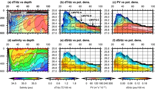
Fig. 2. The 35.5◦S longitudinal section of (a) potential density (black contours; CI=0.1 kg m−3) with dT/dz (colored shade; CI=0.2◦C/100 m) versus depth (m), (b) dT/dz (CI=0.2◦C/100 m) versus potential density (kg m−3), (c) PV (CI=30×10−12m−1s−1) versus potential density (kg m−3), (d) dT/dz (red contours; CI=0.2◦C/100 m) with salinity (colored shade; CI=0.1 psu) versus depth (m), (e) dT/dz (black contours; CI=0.2◦C/100 m) with dS/dz (psu/100 m; colored shade) versus potential density (kg m−3) and (f) PV (black contours; CI=30×10−12m−1s−1) with dS/dz (psu/100 m; colored shade) versus potential density (kg m−3).
IOSTMW (within 25.8–26.2σθ), another mode water (within 26.4–26.7σθ) which we call here “the second subtropical mode water”, and SAMW (within 26.6–26.9σθ).
It is worth mentioning the similarities and differences of the dT/dz, PV and the vertical salinity gradient (dT/dz) distributions along the 35.5◦S line (Fig. 2b–f). First, as a broad picture, the distribution of low dS/dz (less than 0.1 psu/100 m) corresponded to the distribution of low dT/dz (less than 0.8◦C/100 m east of 50◦E, less than 1.0◦C/100 m in 40–50◦E and less than 1.4◦C/100 m in 25–40◦E). This agreement was better than the low PV distribution, since higher dS/dz (higher than 0.1 psu/100 m) sometimes ap-peared in the lower PV region (less than 60×10−12m−1s−1 in 55–80◦E). Second, there were three noticeable differences between the longitudinal dT/dz structure and PV structure probably due to the salinity stratification. While the dT/dz minimum appeared on 25.9–26.1σθ in 30–45◦E, the PV minimum did not appear in these density and longitudinal ranges. This difference may come from the salinity strati-fication (greater than 0.1 psu/100 m) on 26.1–26.4σθ in 30– 40◦E and 26.3–26.4σθ in 40–50◦E. In these areas, temper-ature and salinity compensate each other and they may form relatively homogeneous density stratification below the dT/dz minimum. PV below the dT/dz minimum could become as
25.6
25.8
26.0
26.2
26.4
26.6
26.8
27.0
potential density (kg m
)
0.4 0.8 1.2 1.6 2.0
dT/dz ( C/100 m)
25.6
25.8
26.0
26.2
26.4
26.6
26.8
27.0
0.4 0.8 1.2 1.6 2.0
dT/dz ( C/100 m)
-3
potential density (kg m
)
-3
˚ ˚
40 S 30 S 20 S 10 S
40 S 30 S 20 S 10 S
(a)
(b)
Figure 3
Fig. 3. Relationship between the dT/dz (◦C/100 m) and potential density (kg m−3) in two selected sub-regions. The map shows the locations of Region A (33–38◦S and 28–35◦E) and Region B (33–38◦S and 40–47◦E).
4 Water characteristics of the LMVTG
We selected two sub-regions of the western part of the In-dian Ocean subtropical gyre to characterise the dT/dz struc-ture (Fig. 3): Region A (33–38◦S and 28–35◦E) and Re-gion B (33–38◦S and 40–47◦E). In both sub-regions, each profile contained two LMVTG types: one denser and the other lighter than 26.3σθ. The density range of each type was different in the two sub-regions. In Region A, the denser LMVTG appeared around 26.6–26.7σθ with a dT/dz as low as 1.1◦C/100 m, and the lighter LMVTG around 25.7–26.2σθ had a dT/dz lower than 1.4◦C/100 m. In Re-gion B, the denser LMVTG was around 26.4–26.7σθ and the lighter LMVTG around 26.0–26.2σθ, both with a dT/dz lower than 1.0◦C/100 m. Since the lighter LMVTG
ap-pears as LMVTG A in the 35.5◦S longitudinal dT/dz
sec-tion (Fig. 2b), the lighter LMVTG likely corresponds to the IOSTMW.
Although the lighter LMVTG existed in these sub-regions, we could not extract it objectively by applying any single threshold of dT/dz. As shown in Fig. 3, we could not de-tect the lighter LMVTG in Region A by applying a threshold of 1.0◦C/100 m, which was an appropriate threshold for de-tecting the lighter LMVTG in Region B. The dT/dz of the lighter LMVTG in Region A was higher than 1.0◦C/100 m.
Conversely, we could not detect the lighter LMVTG in Re-gion B by applying a threshold of 1.4◦C/100 m, which was an appropriate threshold for detecting the lighter LMVTG in Region A. The maximum dT/dz below the lighter LMVTG in Region B was lower than 1.4◦C/100 m. This situation is different from that of other subtropical gyres. For example, we can detect the LMVTG corresponding to North Pacific STMW (Masuzawa, 1969; Suga and Hanawa, 1995) in the
western part of the North Pacific subtropical gyre reasonably well by applying any single threshold of dT/dz from 1.0 to 1.8◦C/100 m. It is important to note that this does not sig-nify the vulnerability of the LMVTG; rather, the weak tem-perature stratification below the LMVTG causes difficulty in detecting the LMVTG. If sufficient temperature stratifica-tion (greater than 2.0◦C/100 m) had existed below the lighter LMVTG, we could have detected the lighter LMVTG in both sub-regions A and B reasonably by applying any sin-gle threshold of dT/dz from 1.4 to 2.0◦C/100 m.
We adapted a new method to extract multiple LMVTGs objectively from a single dT/dz profile with weak temper-ature stratification. We changed the threshold of dT/dz continuously from 2.0 to 0.0◦C/100 m, at intervals of 0.02◦C/100 m. Because we also needed to take into account
0
200
400
600
800
Depth (m)
0.4 0.8 1.2 1.6 2.0
dT/dz (˚C/100 m) 0
200
400
600
800
Depth (m)
0.4 0.8 1.2 1.6 2.0
dT/dz (˚C/100 m)
Figure 4
Threshold of dT/dz was changed continuously.
core →
core →
core →
core →
LMVTG
LMVTG
LMVTG LMVTG
Threshold of dT/dz was changed continuously.
(a)
(b)
Fig. 4. A schematic of the method for detecting multiple LMVTGs from a single profile. Two typical dT/dz profiles (◦C/100 m) are shown: (a) 35.5◦S, 32.5◦E and (b) 35.5◦S, 41.5◦E. The dotted line shows the threshold of dT/dz which was varied continuously from 2.0 to 0.0◦C/100 m in 0.02◦C/100 m intervals. Black arrows show the LMVTG detected with a certain dT/dz threshold. Positions of LMVTG core are also shown.
25.6
25.8 26.2
26.8
6 9 12 15 18
Temperature (˚C)
34.0 34.5 35.0 35.5 36.0
Salinity (psu)
Figure 5
(b)
26.6
26
26.4
26.8
27.2
27
2625.8 26.2
26.6 26.4
30˚E 60˚E 90˚E 120˚E 50˚S
40˚S 30˚S 20˚S 10˚S
8 12 16 20
Core temperature (˚C)
(a)
0 2 4 6 8 10
Number
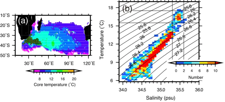
Fig. 5. (a) Spatial distribution of core temperature of LMVTG and (b) occurrence frequency of core water characteristics on the bivariate classes of temperature and salinity in the 10–50◦S, 20–120◦E region. When two cores are detected from a single dT/dz profile, the higher core temperature is plotted on the spatial distribution of core temperature, and both core water characteristics are counted to calculate the occurrence frequency. In (a), core temperatures higher than 15.5◦C are circled by a solid line.
We extracted water characteristics of the LMVTG core from a wide area (10–50◦S, 20–120◦E) of the South Indian
Ocean using this method. Generally, one core was extracted from a single dT/dz profile north of 30◦S, while two cores were extracted on the north side of the STF and west of 70◦E, and on the north side of the SAF and east of 70◦E. Most of the second cores were detected in the density range denser than 26.5σθ. Figure 5a shows that cores colder than 10◦C corresponding to denser SAMW were distributed anti-clockwise around the outer northeastern rim of the subtrop-ical gyre. This characteristic agreed with previous studies (McCarthy and Talley, 1999; Wong, 2005). The core tem-perature was higher than 15.5◦C between 33–38◦S and 25– 50◦E. Figure 5b shows that an area census of the core
tem-perature and salinity reveals two bivariate modes around 8.0– 14.0◦C, 34.3–35.3 psu and denser than 26.3σ
θ, and around 15.5–17.5◦C, 35.3–35.6 psu and lighter than 26.3σθ. The
density and temperature ranges of the denser mode corre-sponded to that of SAMW and MLD C. The density and temperature ranges of the lighter mode corresponded to that of MLD A. Fewer LMVTG cores appeared on the density range of MLD B. It seems that water mass corresponding to MLD B does not subduct into the interior South Indian Ocean for some unknown reasons.
According to previous studies, it is reasonable to assume that the other much broader occurrence frequency maximum of core water characteristics around 8.0–14.0◦C and 34.3–
35.3 psu is due to two mode waters: the second subtropical mode water centered around 12.0–14.0◦C and 35.0–35.4 psu formed north of the STF, and SAMW around 8.0–10.0◦C and 34.2–34.6 psu formed south of the STF. This interpreta-tion is reasonable because the definiinterpreta-tion of the STF (10.0– 12.0◦C and 34.6–35.0 psu at 100 dbar; Orsi et al., 1995) di-vides this broad maximum into two parts through the mid-dle. Although these two mode waters did not appear as two occurrence frequency maxima, the MLD maxima distribu-tion (Fig. 1) and the distribudistribu-tion of dT/dz along 35.5◦S line (Fig. 2a, b) suggested that they are independent mode waters. Therefore, water characteristics of the second subtropical mode water were estimated based on winter mixed layer wa-ter characwa-teristics in September (Fig. 1). Sea-surface wawa-ter characteristics with MLD greater than 200 m, in the 57–75◦E
longitudinal band and north of STF were averaged. The averaged water characteristics and the standard deviations were 12.84±0.57◦C, 35.17±0.11 psu and 26.57±0.04σθ. These averaged water characteristics agreed with McDon-agh et al. (2005) and this density range agreed with that of LMVTG B (Fig. 2b).
We calculated the averaged IOSTMW water character-istics. All core temperatures higher than 15.5◦C were counted. The averaged IOSTMW water characteristics and standard deviations were 16.54±0.49◦C, 35.51±0.04 psu, and 26.0±0.1σθ. According to Bryden et al. (2003), up-per thermocline waters (10.0–17.0◦C) along the 32◦S hy-drographic line showed substantial oscillations during 1936– 2002. To examine the time period that this averaged IOSTMW water property represented, we investigated the source data used to construct the IOHB. The source data ob-tained in the region 30–40◦S and 20–50◦E during January– March were mainly from the period of 1960–2004, with peaks in the 1970s and 1990s. Therefore, we concluded that this averaged water property represented approximately the time period from 1960 to 2004.
The water characteristics of the IOSTMW specified above were compared with those described in previous studies. The temperature specified in the present study was about 1◦C lower than that reported by Olson et al. (1992). The tem-perature difference between our results and theirs was pre-sumably due to the difference in the analysed area. The IOSTMW core temperature varies spatially, as indicated in Fig. 3, with lighter density (higher temp.) values in the west. While the IOSTMW in Region A had a core density of ap-proximately 25.9±0.2σθand a core temperature of approx-imately 17.0±1.0◦C, the IOSTMW in Region B had a core density of approximately 26.1±0.1σθ and a core tempera-ture of approximately 16.5±0.5◦C. We expect our results to represent the IOSTMW water characteristics more accurately because we treated the core temperature more carefully over a wider region of the Indian Ocean subtropical gyre.
5 Spatial distribution of IOSTMW
In this section, we show the limitations of the LMVTG as a tool for describing the spatial extent of IOSTMW and ex-amine the spatial distribution of IOSTMW from a different viewpoint. While the North Pacific Central Mode Water (Nakamura, 1996; Suga et al., 1997) forms LMVTG only in the 35–40◦N, 160◦E–160◦W region, its signature as a lateral minimum of low PV on the 26.4σθ isopycnal surface spreads widely southward down to 20◦N from the forma-tion area along the gyre flow path (Suga et al., 2004). In an area of weakly stratified temperature structure below the mode water, the distribution of the lateral minimum of low PV does not always correspond to the distribution area of the LMVTG.
Figure 6a shows the distribution of PV on the 26.1σθ isopycnal surface, where the IOSTMW water characteristics formed a modal class of temperature and salinity for the area census (Fig. 5b). The lateral minimum of low PV (less than 300×10−12m−1s−1) on the 26.1σθ isopycnal surface was distributed over the 27–38◦S, 25–50◦E region. While the southern part of this low PV corresponded quite well to the distribution area of the LMVTG, the northern part did not. Through careful examination of the northern part, we con-firmed that the 15.5–17.5◦C layer contained dT/dz as low as 1.3◦C/100 m. This layer did not form the LMVTG because no stronger temperature stratification existed below the 15.5– 17.5◦C layer. Since the water mass is generally advected on the isopycnal surface, it is reasonable to consider that the whole region of the lateral minimum of PV is a remnant of the winter mixed layer. Therefore, we concluded that a PV of less than 300×10−12m−1s−1on the 26.1σ
θ isopycnal sur-face represented the IOSTMW region more accurately.
We calculated the thickness of the 15.5–17.5◦C layer which is equivalent to a low PV value of 300×10−12m−1s−1 under some assumptions. The temperature range of 15.5– 17.5◦C corresponded to the IOSTMW core temperature range (Fig. 4b). Assuming that the relative vorticity is negligible and the vertical salinity stratification is fixed, the thickness of the 15.5–17.5◦C layer can be calculated based on Eq. (1)
P V≈ −f ρ
∂ρ ∂z=f
α∂T
∂z −β ∂S ∂z
(1)
ρis the averaged IOSTMW potential density,αis a thermal expansion coefficient, β is a saline contraction coefficient andf is the coriolis parameter. Theαandβwere calculated using the averaged IOSTMW water characteristics, and thef
20 E 40 E 60 E 80 E 40 S
30 S 20 S 10 S
20 E 40 E 60 E 80 E
40 S 30 S 20 S 10 S
0 60 120 180 240 300 PV (10-12m-1s-1)
(a)
20 E 40 E 60 E 80 E
40 S 30 S 20 S 10 S
100 120 140 160
Thickness (m)
(b)
Figure 6
Fig. 6. (a) Distribution of PV (10−12m−1s−1) on the 26.1σθ isopycnal surface. The crosses represent all LMVTG positions with a core temperature higher than 15.5◦C, which are detected by changing the threshold of vertical temperature gradient continuously from 2.0◦C/100 m to 0.0◦C/100 m at 0.02◦C/100 m intervals. (b) The spatial distribution of the thickness of the 15.5–17.5◦C layer greater than 100 m is superimposed on the dynamic height (m2s−2) at 200 m relative to 1000 m.
20 E 40 E 60 E 80 E 100 E 120 E
50 S
40 S
30 S
20 S
10 S
0
20 E 40 E 60 E 80 E 100 E 120 E
50 S
40 S
30 S
20 S
10 S
0 (a) 26.5 σ
θ
Figure 7
20 E 40 E 60 E 80 E 100 E 120 E
50 S
40 S
30 S
20 S
10 S
0
20 E 40 E 60 E 80 E 100 E 120 E
50 S
40 S
30 S
20 S
10 S
0 (c) 26.7 σ
θ
20 E 40 E 60 E 80 E 100 E 120 E
20 E 40 E 60 E 80 E 100 E 120 E
(b) 26.6 σθ
20 E 40 E 60 E 80 E 100 E 120 E
20 E 40 E 60 E 80 E 100 E 120 E
(d) 26.8 σθ
0 60 120 180 240 300 PV (10-12m-1s-1)
this assumption, the calculated thickness was 97±18 m. The uncertainty came mainly from the variation of the corio-lis parameter. The area where the 15.5–17.5◦C layer was
greater than 100 m corresponded fairly well to the distribu-tion area of low PV less than 300×10−12m−1s−1 on the 26.1σθ isopycnal surface (Fig. 6b). Thus, we suggest that the area of the 15.5–17.5◦C layer greater than 100 m roughly represents the IOSTMW distribution area.
6 Conclusions
We have improved the basic description (water charac-teristics and spatial distribution) of the IOSTMW using an isopycnally averaged three-dimensional hydrographic dataset. Following the STMW definition of Hanawa and Talley (2001), we defined the IOSTMW as the mode wa-ter adjacent to the Agulhas currents with single mode of water characteristics. From this point-of-view, we clarified the relationships between several mode waters in the In-dian Ocean subtropical gyre (north of STF). As reported by previous studies, two mode waters and their corresponding MLD maxima were observed north of the STF: IOSTWM (within 25.8–26.2σθ) in 28–45◦E and a second subtropical mode water in the subtropical gyre (within 26.4–26.7σθ) in the 60–80◦E longitudinal band. We found that we could not detect the whole IOSTMW as an LMVTG using any single dT/dz threshold because temperature stratification be-low the IOSTMW was weak. By changing the threshold of dT/dz continuously, we confirmed that a substantial mass of LMVTG was located in the western part of the Indian Ocean subtropical gyre and that its core water characteristics formed a mode on the bivariate classes of temperature and salinity for the area census. Thus, we concluded that this mass of LMVTG corresponds to IOSTMW. The averaged water char-acteristics of the IOSTMW approximately during 1960–2004 were 16.54±0.49◦C, 35.51±0.04 psu and 26.0±0.1σθ. The temperature of the IOSTMW was about 1◦C lower than that reported in previous studies. The IOSTMW was dis-tributed in 25–50◦E, 27–38◦S. This area had a lateral min-imum of low PV (less than 300×10−12m−1s−1) on the 26.1σθ isopycnal surface where the IOSTMW water char-acteristics formed a mode on the bivariate classes of temper-ature and salinity. The IOSTMW distribution area was also approximated as the area where the thickness of the 15.5– 17.5◦C layer was greater than 100 m. The formation region
and approximate water characteristics of the second subtrop-ical mode water in the subtropsubtrop-ical gyre were also presented. Its probable formation region was 37–42◦S and 60–80◦E in longitudinal band and north of the STF. Its approximate water characteristics were 12.84±0.57◦C, 35.17±0.11 psu and 26.57±0.04σθ.
Figure 7 shows the distribution of PV on 26.5–26.8σθ isopycnal surfaces based on the summer averaged IOHB dataset in order to illustrate how these different layers may
be ventilated in the South Indian Ocean subtropical gyre for future studies. The positions of LMVTG thicker than 200 m within 26.45–26.55σθ are also plotted on 26.5σθ isopycnal surfaces. A thicker thickness criterion was ap-plied because typical vertical scales of the thermostat in this density range (denser than 26.4σθ) are larger than that of the IOSTMW density range (Fig. 2a). Low PV (less than 120×10−12m−1s−1) on the 26.5σθ isopycnal surfaces spreads anticlockwise in the southwestern part of the Indian Ocean subtropical gyre from its winter outcrop area, while low PV (less than 60×10−12m−1s−1) on the 26.8σθsurface (denser SAMW) spreads anticlockwise along the northeast-ern rim of Indian Ocean subtropical gyre from their forma-tion region. The correspondence between the posiforma-tions of LMVTG and low PV distribution on each isopycnal layer suggests that these low PV distributions represent the flow path of the remnant winter deep mixed layer. Therefore, we suggest that the second subtropical mode water may venti-late in the southwestern part of the Indian Ocean subtrop-ical gyre. However, the relationship between the positions of LMVTG and low PV distribution and the relationship to the flow field should be examined carefully. As shown in Fig. 2b and 2c, the PV minimum on 26.5–26.7σθ in 50– 70◦E appeared deeper than the depth of the dT/dz minimum by around 0.1σθ. Using the Argo data, the SODB and an ocean general circulation model, new studies about South In-dian Ocean ventilation are in progress (Sallee et al., 2009; Koch-Larrouy et al., 2009). Detailed examination and inter-pretation will be left for future studies.
Acknowledgements. Mixed layer data calculated from the Argo data and the SODB was provided by Jean-Baptiste Sallee. The comments from two anonymous referees have improved this paper. This study was performed as a part of the 21st Century Center-of-Excellence (COE) Program “Advanced Science and Technology Center for Dynamic Earth (E-ASTEC)” at Tohoku University.
Edited by: A. J. George Nurser
References
Akima, H.: A new method of interpolation and smooth curve fitting based on local procedures, J. Assoc. Comput. Math., 17, 589– 602, 1970.
Aoki, S., Hariyama, M., Mitsudera, H., Sasaki, H., and Sasai, Y.: Formation regions of Subantarctic Mode Water detected by OFES and Argo profiling floats, Geophys. Res. Lett., 34, L10606, doi:10.1029/2007GL029828, 2007.
Boyer, T. P., Stephens, C., Antonov, J. I., Conkright, M. E., Lo-carnini, R. A., O’Brien, T. D., and Garcia, H. E.: World Ocean Atlas 2001, Vol. 2, Salinity, NOAA Atlas NESDIS 50, CD-ROM., 2002.
Fine, R. A.: Circulation of Antarctic Intermediate Water in the South Indian-Ocean, Deep-Sea Res., 40, 2021–2042, 1993. Hanawa, K. and Sugimoto, S.: “Reemergence” areas of winter sea
surface temperature anomalies in the world’s oceans, Geophys. Res. Lett., 31, L10303, doi:10.1029/2004GL01904, 2004. Hanawa, K. and Talley, L. D.: Mode Waters, Ocean Circulation
and Climate, in: Observing and Modelling the Global Ocean, edited by: Siedler, G., Church, J., and Gould, J., Academic Press, London, 373–386, 2001.
Kobayashi, T. and Suga, T.: The Indian Ocean HydroBase: A high-quality climatological dataset for the Indian Ocean, Prog. Oceanogr., 68, 75–114, 2006.
Koch-Larrouy, A., Morrow, R., Penduff, T., and Juza, M.: Ori-gin and mechanism of Sub Antarctic Mode Water formation and transformation in the Southern Indian Ocean, Ocean Dynamics, in revision, 2010.
Marshall, J. C., Nurser, A. J. G., and Williams, R. G.: Inferring the Subduction Rate and Period over the North-Atlantic, J. Phys. Oceanogr., 23, 1315–1329, 1993.
Masuzawa, J.: Subtropical mode water, Deep-Sea Res., 16, 453– 472, 1969.
McCarthy, M. C. and Talley, L. D.: Three-dimensional isoneutral potential vorticity structure in the Indian Ocean, J. Geophys. Res., 104(C6), 13251–13267, 1999.
McCartney, M. S.: Subantarctic Mode Water, A Voyage of Dis-covery, in: George Deacon 70th Anniversary Volume, edited by: Angel, M., Pergamon Press, Oxford 103–199, 1977.
McCartney, M. S.: The subtropical recirculation of mode waters., J. Mar. Res., 40 (Suppl.), 427–464, 1982.
McDonagh, E. L., Bryden, H. L., King, B. A., Sanders, R. J., Cun-ningham, S. A., and Marsh, R.: Decadal changes in the south Indian Ocean thermocline, J. Climate, 18, 1575–1590, 2005. Nakamura, H.: A pycnostad on the bottom of the ventilated
por-tion in the central subtropical North Pacific: Its distribupor-tion and formation, J. Oceanogr., 52, 172–188, 1996.
Olson, D. B., Fine, R. A., and Gordon, A. L.: Convective mod-ification of water masses in the Agulhas?, Deep-Sea Res., 39, S163–S181, 1992.
Orsi, A. H., Whitworth, T., and Nowlin, W. D.: On the Meridional Extent and Fronts of the Antarctic Circumpolar Current, Deep-Sea Res., 42, 641–673, 1995.
Ridgway, K. R., Dunn, J. R., and Wilkin, J. L.: Ocean interpola-tion by four-dimensional weighted least squares – applicainterpola-tion to the waters around Australasia, J. Atmos. Oceanic Technol., 19, 1357–1375, 2002.
Rintoul, S. R. and England, M. H.: Ekman transport dominates air– sea fluxes in driving variability of Subantarctic Mode Water, J. Phys. Oceanogr., 32, 1308–1321, 2002.
Sallee, J. B., Speer, K., and Morrow, R.: Response of the Antarctic Circumpolar Current to atmospheric variability, J. Climate, 21, 3020–3039, 2008.
Sallee, J. B., Speer, K., Rintoul, S. R. and Wijffels, S.: Southern Ocean thermocline ventilation, J. Phys. Oceanogr., doi:10.1175/2009JPO4291.1, 2010.
Sallee, J. B., Wienders, N., Speer, K., and Morrow, R.: Formation of subantarctic mode water in the southeastern Indian Ocean, Ocean Dynamics, 56, 525–542, 2006.
Stephens, C., Antonov, J. I., Boyer, T. P., Conkright, M. E., Lo-carnini, R. A., O’Brien, T. D., and Garcia, H. E.: World Ocean Atlas 2001, Vol. 1, Temperature, NOAA Atlas NESDIS 49, CD-ROM., 2002.
Suga, T. and Hanawa K.: The Subtropical Mode Water Circulation in the North Pacific, J. Phys. Oceanogr., 25, 958–970, 1995. Suga, T., Motoki, K., Aoki, Y., and Macdonald, A. M.: The North
Pacific climatology of winter mixed layer and mode waters, J. Phys. Oceanogr., 34, 3–22, 2004.
Suga, T., Takei, Y., and Hanawa, K.: Thermostad Distribution in the North Pacific Subtropical Gyre: The Central Mode Waters and the Subtropical Mode Water, J. Phys. Oceanogr., 27, 140– 152, 1997.
Toole, J. M. and Warren, B. A.: A hydrographic section across the south Indian-Ocean, Deep-Sea Res., 40, 1973–2019, 1993. Wong, A. P. S.: Subantarctic Mode Water and Antarctic