https://doi.org/10.5194/npg-25-1-2018
© Author(s) 2018. This work is distributed under the Creative Commons Attribution 4.0 License.
On the interaction of short linear internal waves with
internal solitary waves
Chengzhu Xu and Marek Stastna
Department of Applied Mathematics, University of Waterloo, Waterloo, Ontario N2L 3G1, Canada Correspondence:Chengzhu Xu (c2xu@uwaterloo.ca)
Received: 31 August 2017 – Discussion started: 12 September 2017
Revised: 30 November 2017 – Accepted: 3 December 2017 – Published: 17 January 2018
Abstract. We study the interaction of small-scale internal wave packets with a large-scale internal solitary wave us-ing high-resolution direct numerical simulations in two di-mensions. A key finding is that for wave packets whose con-stituent waves are short in comparison to the solitary wave width, the interaction leads to an almost complete destruction of the short waves. For mode-1 short waves in the packet, as the wavelength increases, a cutoff is reached, and for larger wavelengths the waves in the packet are able to maintain their structure after the interaction. This cutoff corresponds to the wavelength at which the phase speed of the short waves up-stream of the solitary wave exceeds the maximum current in-duced by the solitary wave. For mode-2 waves in the packet, however, no corresponding cutoff is found. Analysis based on linear theory suggests that the destruction of short waves occurs primarily due to the velocity shear induced by the soli-tary wave, which alters the vertical structure of the waves so that significant wave activity is found only above (below) the deformed pycnocline for overtaking (head-on) collisions. The deformation of vertical structure is more significant for waves with a smaller wavelength. Consequently, it is more difficult for these waves to adjust to the new solitary-wave-induced background environment. These results suggest that through the interaction with relatively smaller length scale waves, internal solitary waves can provide a means to de-crease the power observed in the short-wave band in the coastal ocean.
1 Introduction
Internal waves are commonly observed in stably stratified fluids such as the Earth’s atmosphere and oceans. They ex-ist in a variety of environmental conditions, including those with background shear currents, and on different length and timescales. The interaction between internal waves and other physical processes results in energy exchange between the waves and the background environment (Sarkar and Scotti, 2017). Based on linear wave theory, Cai et al. (2008) studied internal waves in a shear background current, and found that in addition to the velocity shear across the pycnocline, the vertical structure of the horizontal velocity profile also had a significant influence on the evolution of internal waves. The interaction between mode-1 internal tides and mesoscale ed-dies was examined in Dunphy and Lamb (2014). The authors found that the interaction, essentially the bending of the paths followed by the wave energy, produced hot and cold spots of energy flux. These took the form of beam-like patterns, and resulted in the scattering of energy from the incident mode-1 to modes-2 and higher. The above-mentioned studies were not dependent on the presence of boundaries. Motivated by the fact that internal waves have reflection properties that are different from classical Snell’s law, Grisouard and Thomas (2015) investigated the interaction between near-inertial waves and ocean fronts, and found that near-inertial waves could travel with two distinct characteristics at a front, one flat and one tilted upward, implying the existence of critical reflections from the ocean surface.
induced by the relatively larger length scale wave, as they interact with each other. Previous literature has considered wave–wave interaction in a variety of contexts. For exam-ple, using ray theory for linearized waves and the principle of wave action conservation, Broutman and Young (1986) studied the interaction of short high-frequency progressive internal waves and long progressive near-inertial waves, and found that there was a net energy transfer from the iner-tial wave field to the short internal waves. Lamb (1998) in-vestigated the interaction between two mode-1 internal tary waves (ISWs), and showed that the interaction of soli-tary waves did not correspond to soliton dynamics, since energy exchange was observed and small-amplitude trailing waves of possibly higher modes were generated. More re-cently, Stastna et al. (2015) examined the interaction between mode-1 and mode-2 internal solitary (solitary-like in cases when the mode-2 wave was breaking) waves, and demon-strated that the interaction yielded a nearly complete disinte-gration of the relatively smaller mode-2 wave. In particular, the majority of kinetic energy carried by the mode-2 wave was lost and the disturbance to the flow field after the col-lision no longer had a mode-2 structure. When the length scales of participating waves are similar, Sutherland (2016) found that nonlinear self-interaction might occur, which re-sulted in energy being transferred to superharmonic distur-bances. These disturbances were a superposition of modes such that the amplitude was largest where the change in back-ground buoyancy frequency with depth was largest.
In this work, we study the interaction of small-scale mode-1 internal waves initialized from linear waves with an ISW initialized from the exact Dubreil–Jacotin–Long equa-tion, using high-resolution direct numerical simulations in two dimensions. Internal waves that are short in terms of wavelength compared to the fluid depth are generally less documented in the nonlinear wave literature. In fact, the derivation of the model equations of most weakly nonlin-ear theories, such as the Korteweg–de Vries equation and its variations, assumes large horizontal scales and thus filters out short waves (Lamb and Yan, 1996). Nevertheless, such waves occupy a non-negligible portion of the Garrett–Munk spec-trum of internal waves in the oceans (Thorpe, 2005), and it is important to understand their behaviour in order to fully describe internal wave dynamics.
The remainder of the paper is organized as follows: the-oretical descriptions of internal waves are introduced in Sect. 2. The problem is formulated in Sect. 3. The simula-tion results are presented in Sect. 4. A key finding is that for waves that are short in comparison to the ISW width, the in-teraction leads to an almost complete destruction of the short waves; for mo1 short waves, however, there is a cutoff de-termined by the wavelength of short waves, and waves longer than this cutoff maintain their structure after interaction. We show that this is a key difference from mode-1–mode-2 in-teraction, which is examined in Stastna et al. (2015). The en-ergy transfer during the interaction is discussed in Sect. 5,
and a summary concluding the findings of this study is given in Sect. 6.
2 Internal wave theories
In the classical linear theory, the horizontal structure of inter-nal waves is usually described by the travelling wave ansatz exp(ik[x−cp(k)t])wherekis the horizontal wave number
and is related to the wavelengthλby the formulak=2π/λ, andcpis the phase speed. The vertical structure is described
by solutions of the eigenvalue problem often referred to as the Taylor–Goldstein (TG) equation (Kundu et al., 2012), which is given by
φzz+
N2(z)
(cp−U )2
+ Uzz cp−U
−k2
φ=0,
φ (0)=φ (H )=0, (1) whereU=U (z)is the background horizontal velocity,N is the buoyancy frequency defined by
N2(z)= −dρ¯
dzg, (2)
withρ¯ being the (dimensionless) undisturbed density pro-file in the background andH is the height of the water col-umn. If there are no critical layers (i.e.cp−U6=0 for allz),
for physically relevantN (z), the TG equation has an infi-nite set of discrete eigenvaluescp which decrease ask
in-creases and as the mode number inin-creases. The correspond-ing eigenfunctionφ (z)characterizes the vertical structure of the velocity field (e.g. the wave-induced horizontal velocity is proportional toφz). It also determines the mode number of
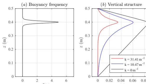
internal waves according to the formula “one plus the num-ber of zeros that the eigenfunction has in the interior of the water column”. Note that the TG equation simplifies consid-erably when there is no background shear flow. An exam-ple of a single pycnocline buoyancy frequency profile, to-gether with the corresponding vertical structure functions for mode-1 waves of particular horizontal wave numbers in the absence of a shear current, is given in Fig. 1.
Due to the nonlinear nature of fluid flows, purely linear waves are a mathematical idealization. For large-amplitude waves or on timescales long enough for nonlinear effects to manifest themselves, results predicted by the linear theory do not agree with measurements. Weakly nonlinear theory attempts to better describe internal wave dynamics by ex-panding flow variables asymptotically and retaining correc-tions that correspond to finite amplitude (nonlinearity) and wavelength (dispersion). The most famous weakly nonlinear model is probably the Korteweg–de Vries (KdV) equation, given by (Lamb, 2005),
Bt+clwBx+αBBx+βBxxx=0, (3)
0 0.02 0.04 0.06 0.08 0
0.1 0.2 0.3 0.4 0.5
k = 31.41 m-1
k = 10.47 m-1 k = 0 m-1
0 2 4 6
0 0.1 0.2 0.3 0.4 0.5
Figure 1.Example of(a)buoyancy frequency profile and(b)vertical structure profiles as the wave number varies for mode-1 internal waves in a zero-background current. The amplitudes of the eigenfunctions have been varied for clarity of visual presentation.
is the speed of linear long wave (i.e. waves withk=0), and the parametersαandβmeasures the nonlinearity and disper-sion of the wave, respectively. Analysis of the KdV equation shows that it has solitary wave solutions of the form B(x, t )=asech2
x−V t
λ
, (4)
wherea measures the wave amplitude andV is the nonlin-ear wave propagation speed. Internal solitary waves (ISWs) are translating waves of permanent form, which consist of a single wave crest. They are one of the most commonly ob-served types of internal waves in the field (e.g. Klymak and Moum, 2003; Scotti and Pineda, 2004; also see Helfrich and Melville, 2006, for a more complete review).
While the KdV theory correctly predicts some properties of internal waves, it can only be expected to perform well within certain asymptotic limits (e.g. the small-amplitude limit and long-wave limit). For large-amplitude waves, so-lutions of the KdV equation and its variations have been shown to be different from waveforms predicted by the fully nonlinear theory (Lamb and Yan, 1996; Lamb, 1999). Fully nonlinear ISWs can be computed by solving the nonlin-ear eigenvalue problem known as the Dubreil–Jacotin–Long (DJL) equation, which, in a zero-background current, takes the form (Stastna and Lamb, 2002; Lamb, 2005)
∇2η+N
2(z−η)
c2isw η =0, η(x,0)=η(x, H )=0,
η(x, z)→0 asx→ ±∞. (5)
In this equation,ciswis the solitary wave propagation speed
(equivalent toV in the KdV theory), andη=η(x, z)is the vertical displacement of the isopycnal relative to its far-upstream depth. The DJL equation is equivalent to the full set of stratified Euler equations in a frame moving with the wave,
where no assumptions are made with respect to the nonlin-earity of the fluid flow. Hence, its solutions are exact soli-tary wave solutions. For non-constantN, the DJL equation has no analytical solutions. In this work, the DJL equation is solved numerically using the method described in Dun-phy et al. (2011). The algorithm for solving the DJL equa-tion is based on the variaequa-tional scheme developed in Turk-ington et al. (1991), which iteratively seeks a solution that minimizes the kinetic energy, subject to the constraint that the scaled available potential energy is held fixed.
3 Problem formulation
3.1 Governing equations and numerical method The governing equations for the present work are the incom-pressible Navier–Stokes equations under the rigid lid and Boussinesq approximations, given by (Kundu et al., 2012) Du
Dt = −∇p−ρg ˆ
k+ν∇2u, (6a)
∇ ·u=0, (6b)
Dρ Dt =κ∇
2ρ, (6c)
where D/Dtis the material derivative defined by D
Dt = ∂
∂t+u· ∇, (7)
and ∇ =
∂ ∂x,
∂ ∂z
. (8)
ISW domain Lisw
Linear wave domain Llin
0 1 2 3 4 5 6 7 8 9 10
x (m) 0
0.1 0.2 0.3 0.4 0.5
z
(m
)
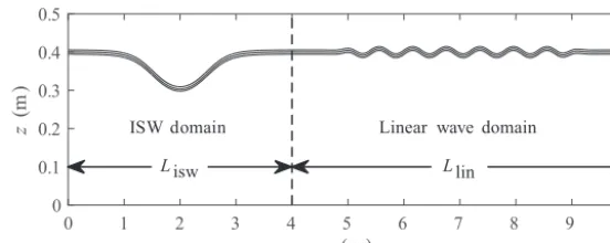
Figure 2.Graph of the model setup. Solid curves are isopycnals indicating the ISW and the linear waves in the initial field.
is the gravitational acceleration, kˆ is the unit vector in the vertical direction (positive upwards),νis the kinematic vis-cosity, andκ is the molecular diffusivity. As is the common practice under the Boussinesq approximation, the equations are in dimensional form, except that the densityρand pres-surepare scaled by the reference densityρ0. For all
simu-lations, we fix the viscosity atν=10−6m2s−1and the dif-fusivity atκ=2×10⁻⁷m2s−1. This gives a Schmidt num-berSc =ν/κ=5. Periodic boundary conditions are used in the horizontal direction, and free-slip boundary conditions are used at the top and bottom boundaries. We note that no-slip conditions have also been tested but the difference is in-significant, since the majority of the velocity perturbations are found near the pycnocline. The effect of the Earth’s rota-tion is neglected, and hence the simularota-tions are performed in an inertial frame of reference.
A complete description of the numerical model used in this study can be found in Subich et al. (2013), where a de-tailed validation and accuracy analysis through several test cases is also given. The model employs a spectral colloca-tion method, which yields highly accurate results at moderate grid resolutions. From a purely numerical point of view, the spectral method requires a minimum of two points in the hor-izontal direction in order to completely resolve a wave (Tre-fethen, 2000). Nevertheless, in this study we employ high resolution in order to better resolve the thin pycnocline, with at least 10 grid points in the pycnocline and across the short waves. For spatial discretization, equally spaced grid points are used in both horizontal and vertical directions. As appro-priate for the boundary conditions, the Fourier transform is applied in the x direction, whereas the Fourier sine or co-sine transform is applied in thezdirection depending on the variable of interest. For time stepping, the model employs an adaptive third-order multistep method, where viscous and diffusive terms are solved implicitly, and pressure is com-puted via operator splitting.
3.2 Model setup and parameter space
A graph showing the model setup is given in Fig. 2, where a right-handed Cartesian coordinate system is considered
with the origin fixed at the lower left corner of the domain. The position vector is expressed asx=(x, z), with thexaxis directed to the right along the flat bottom and thezaxis point-ing up towards the surface. The two-dimensional, rectangu-lar computational domain is on the laboratory scale and has an overall lengthLx=10 m and a depthLz=0.5 m. It
con-sists of an ISW subdomain of lengthLisw=4 m and a
lin-ear wave subdomain of lengthLlin=6 m. The grid size is
Nx×Nz=4096×512, which gives a horizontal grid
spac-ing of 2.44 mm and a vertical grid spacspac-ing of 0.98 mm. We focus on flows in a quasi-two-layer stratification with a dimensionless density difference1ρ=0.01, for which the Boussinesq approximation can be safely adopted. The back-ground density profile, non-dimensionalized by the reference densityρ0, is given by
¯
ρ(z)=1−0.51ρtanh z−z
0
d
, (9)
wherez0is the location of the pycnocline andd is the
half-width of the pycnocline. The specific location of the pycno-cline does not affect the dynamics of the interaction between the ISW and the linear waves in general, except for the case where the pycnocline is close to the surface such that the ISW could be breaking (Lamb, 2002, 2003). In this work, we setz0=0.4 m in order to avoid this situation. The thickness
of the pycnocline can affect the gradient Richardson number through the buoyancy frequency profile it determines, which may have an impact on the interaction. However, this topic is not the focus of the present work (see Sect. 6). In this work, we simply setd=0.01 m for all simulations.
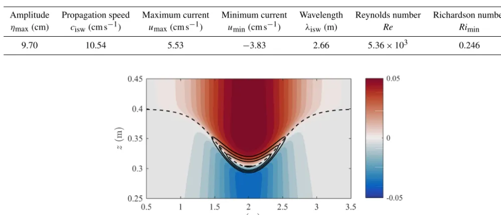
The initial solitary wave is specified by interpolating a so-lution of the DJL equation onto the ISW subdomain. Pa-rameters of the particular solitary wave solution considered in this work are given in Table 1. Here, we compute the Reynolds numberRebased on the amplitude and maximum wave-induced current as
Re=umaxηmax
ν . (10)
Table 1.Solitary wave parameters. Here, the amplitude is measured by the maximum isopycnal displacementηmax, and the wavelength is measured by the horizontal velocity profile along the inviscid upper boundary according to the formulaλisw=2(xR−xL), wherexRandxL satisfy the equationu(xR, Lz)=u(xL, Lz)=0.5umax.
Amplitude Propagation speed Maximum current Minimum current Wavelength Reynolds number Richardson number
ηmax(cm) cisw(cm s−1) umax(cm s−1) umin(cm s−1) λisw(m) Re Rimin
9.70 10.54 5.53 −3.83 2.66 5.36×10³ 0.246
Figure 3.Filled contours showing the horizontal velocity induced by the ISW, with positive current shown in red and negative current shown in blue. The dashed curve shows the isopycnal displacement along the pycnocline. The black contours show the gradient Richardson number withRi=0.25, 0.4, 0.6, and 1 from inside to outside.
the length and velocity scales set by the ISW. The gradient Richardson numberRiis defined by
Ri=N
2
u2 z
, (11)
whereuis the ISW-induced horizontal current, andRiminis
the local minimum of the Richardson number. It measures the ratio between the strength of the stratification and the shear stress in a parallel shear flow. The horizontal velocity profile of the ISW, together with the Richardson number contours, is shown in Fig. 3. The figure shows that the Richardson number has a local minimum in the high-shear region across the pycnocline along the wave crest, and is very large out-side this region. We note that whileRimingiven in Table 1 is
slightly smaller than the critical Richardson number 0.25, the Richardson number criterionRi<0.25 is a necessary but not sufficient condition for linear stability in a parallel shear flow. Moreover, due to the fact that ISW-induced flow is not nec-essarily a parallel shear flow, the onset of shear instability is possible only whenRiis considerably smaller than 0.25 over a region long enough for perturbations to amplify in space (Lamb and Farmer, 2011). Thus, the onset of shear instabil-ity is not likely to occur.
We perform a suite of simulations in which the solitary wave propagates to the right and interacts with a small-scale wave packet initialized from linear waves. The linear waves are specified by solving the TG equation numerically us-ing a pseudo-spectral technique (Trefethen, 2000) in the
lin-ear wave subdomain. In order to ensure a smooth transition across the boundaries between the ISW subdomain and the linear wave subdomain, an envelope function is applied to the amplitude of linear waves. The particular form of the en-velope function used here is given by
env(x)=0.5 tanh
x−(L
isw+1)
0.2
−0.5 tanh
x−(L
x−1)
0.2
, (12)
although by testing other forms we found that results are not sensitive to the exact shape of the envelope.
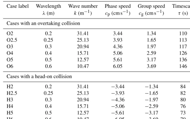
Table 2.Linear wave parameters. In the case labels, O indicates an “overtaking” collision and H indicates a “head-on” collision, and the proceeding digits correspond to the wavelength of the linear waves.
Case label Wavelength Wave number Phase speed Group speed Timescale λ(m) k(m−1) cp(cm s−1) cg(cm s−1) τ(s)
Cases with an overtaking collision
O2 0.2 31.41 3.44 1.34 110
O2.5 0.25 25.13 3.93 1.65 113
O3 0.3 20.94 4.36 1.97 117
O4 0.4 15.71 5.06 2.59 126
O5 0.5 12.57 5.61 3.17 136
O6 0.6 10.47 6.05 3.69 146
Cases with a head-on collision
H2 0.2 31.41 −3.44 −1.34 84
H2.5 0.25 25.13 −3.93 −1.65 82
H3 0.3 20.94 −4.36 −1.97 80
H4 0.4 15.71 −5.06 −2.59 76
H5 0.5 12.57 −5.61 −3.17 73
H6 0.6 10.47 −6.05 −3.69 70
Figure 5.Same as Fig. 4 but for O6. Vertical lines in panels(c)and(d)show the misalignment of wave crests in the two density fields.
For each experiment, we measure the time,τ, over which the solitary wave (which moves at the speedcisw) and the linear
wave packet (which moves at the speedcg) experience a full
collision cycle by defining τ = Lx
cisw−cg
. (13)
Att=τ, the location of the solitary wave relative to the lin-ear wave packet is approximately the same as it was in the initial field. In all figures presented in this paper, reported timeT is scaled by this quantity such thatT =t /τ.
We would like to mention that these linear waves are in fact not purely linear during the simulations. However, by scaling the relevant terms (i.e.BtandBBx) in the KdV
equa-tion (Eq. 3) using the amplitudes and wavelengths of these waves, we found that the timescale at which the nonlinear-ity becomes important is on the order of 1000 s, at least for waves with an amplitude of 1 cm and a wavelength larger than 0.2 m. In contrast, the timescale of the interaction, as indicated in Table 2, is on the order of 100 s. Hence, for clar-ity of notation, the small-scale waves will still be referred to as “linear waves”, as opposed to the “solitary wave” or the “ISW”, in the remainder of this paper.
4 Simulation results 4.1 Evolution of flow fields
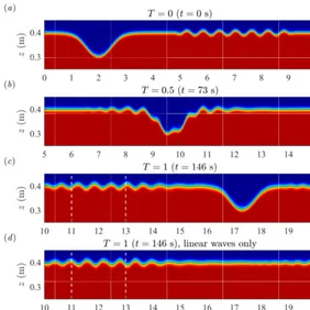
An impression of the overall flow behaviour in the case O2 can be gained from Fig. 4. The initial density profile is shown in Fig. 4a, where the disparity in both amplitude and length scale between the solitary wave and the linear waves can be clearly seen. The linear waves have an amplitude that is ap-proximately 10 % of the solitary wave and a wavelength of 7.5 % of the solitary wave. Figure 4b shows that as the lin-ear waves pass through the solitary wave, they are deformed significantly such that they have lost their coherent, wave-like structure almost entirely. Figure 4c shows that after the collision, the disturbance behind the solitary wave has a spa-tial structure that is completely different from the inispa-tial lin-ear waves. To demonstrate that such deformation of linlin-ear waves does not occur naturally but is a result of the collision, we performed an additional simulation with the same linear wave packet but without the solitary wave. The resulting den-sity field atT =1 is shown in Fig. 4d.
Figure 6.Detailed density contours of the simulations(a)O2 and(b)H2, showing the overturning of the linear waves during the collision.
0 0.5 1
Mode structure 0
0.1 0.2 0.3 0.4 0.5
z
(m
)
(a ) Wavelengt h = 0.2 m
Initial state Overtaking No shear Head-on
0 0.5 1
Mode structure 0
0.1 0.2 0.3 0.4
0.5 (b) Wavelengt h = 0.6 m
Initial state Overtaking No shear Head-on
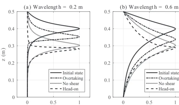
Figure 7.Vertical structure profiles of the linear waves with wavelengths of(a)0.2 m and(b)0.6 m in the initial, undisturbed state (solid curve) and the ISW-induced background state with an overtaking collision (dot-dashed curve), a head-on collision (dashed curve), and a hypothetical zero-background current (dotted curve).
and c show, however, that unlike in the previously discussed case, the linear waves are able to retain their spatial structure throughout the collision. The amplitude is also maintained, suggesting that energy loss during the collision is small. In-stead, comparison to Fig. 5d, which shows the correspond-ing density profile obtained from the simulation with linear waves only, suggests that the primary effect of the collision on the linear waves is a phase shift, as indicated by the ver-tical lines. We will revisit the energy loss in these cases in Sect. 5.
4.2 Destruction of short waves
In Fig. 6, we show details of the density field during the overtaking collision in case O2 (Fig. 6a), and compare it with the density field during the head-on collision in case H2 (Fig. 6b). In both cases, the linear waves in front of the
solitary wave are unperturbed, whereas those behind the tary waves are almost completely destroyed. Inside the soli-tary wave, the deformation of linear waves in the two cases proceeds in a qualitatively different manner. Figure 6a shows that for the overtaking case, overturning of the linear waves occurs above the pycnocline centre, while Fig. 6b shows that for the head-on collision case, overturning occurs with and below the pycnocline.
Figure 8.Detailed density contours showing the mode-2 wave packet(a)before and(b)after the collision with the solitary wave.
an undisturbed situation, and a horizontal velocity with sig-nificant shear across the deformed pycnocline. We then com-puted the linear wave solution with a wavelength of 0.2 m in this background environment using the TG equation (Eq. 1), and compared it with the solution in the undisturbed back-ground environment. The mode structure functions of these solutions are plotted in Fig. 7a. This figure shows that the vertical structure of the horizontal velocity induced by lin-ear waves is highly dependent on the stratification and the background current, such that for both overtaking and head-on collisihead-on cases, the structure functihead-ons at the solitary wave crest (indicated by dashed and dot-dashed curves) are com-pletely different from their initial, undisturbed state (indi-cated by the solid curve). The locations of maximum am-plitude of the structure functions are shifted downward from their undisturbed situation, in order for the linear waves to adapt to the new solitary-wave-induced background strati-fication. However, there is a qualitative difference between the overtaking and head on collision as well. Indeed, un-der the influence of the shear background current, the struc-ture function in the overtaking (head-on) collision case has its maximum value above (below) the disturbed pycnocline. This is consistent with the observation in Fig. 6 that inside the solitary wave, perturbations in the overtaking (head-on) collision case have a wave-like structure above (below) the pycnocline. We also note that if there is no velocity shear in the background, the vertical structure of linear waves of a given wavelength (e.g.λ=0.2 m in this case, as indicated by the dotted curve) depends only on the stratification, re-gardless of the direction they propagate in. Moreover, the vertical structure with respect to the pycnocline centre is es-sentially unchanged. This suggests that the velocity shear in the background alters the vertical structure of the short waves in a nonlinear manner and leads to the observation that a head-on collision manifests differently from an overtaking collision.
In Fig. 7b, we made the same plot for linear waves with a wavelength of 0.6 m. The figure shows that the key dif-ference in the initial structure function is that it has a non-negligible value over a much larger vertical extent. As a re-sult, near the pycnocline centre, changes in the vertical struc-ture functions are much less dramatic in both the overtak-ing and head-on collision cases. Therefore, longer waves are able to adapt to the ISW-induced background environment more easily and hence are more likely to survive the collision with the solitary wave. We also note that formally changing the amplitude of linear waves does not change their vertical structures and thus does not affect the dynamics of the col-lision process, though in practice larger amplitude waves are expected to have a different (i.e. Stokes wave) structure. 4.3 Comparison of mode-1 to mode-2 collisions
The above analysis suggests that as the linear waves en-ter into the solitary-wave-induced background state, they are subject to a modified stratification and a velocity shear due to solitary-wave-induced current, and it is this velocity shear across the deformed pycnocline that leads to the deformation of short waves. This process is in many ways similar to that found in Stastna et al. (2015). However, a key difference is that the disintegration of mode-2 waves due to the collision is much less dependent on their wavelength. To compare and contrast with their results, we performed an additional sim-ulation, with mode-2 waves of amplitude of 1 cm and wave-length of 0.6 m interacting with the same ISW with an over-taking collision. The phase and group speeds of the mode-2 waves are cp=1.43 cm s−1 and cg=1.35 cm s−1,
respec-tively, much smaller than their mode-1 counterparts. Figure 8 shows that after the collision with the ISW, the mode-2 waves are almost completely destroyed, except for some mode-1-like disturbances found nearx=8 m in Fig. 8b.
-1 -0.5 0 0.5 1
Mode structure
0 0.1 0.2 0.3 0.4 0.5
z
(m
)
(a ) Wavelengt h = 0.2 m
Overtaking No shear Head-on
-1 -0.5 0 0.5 1
Mode structure
0 0.1 0.2 0.3 0.4
0.5 (b) Wavelengt h = 0.6 m
Overtaking No shear Head-on
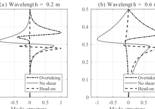
Figure 9.Same as Fig. 7 but for mode-2 waves.
The figure shows that the presence of velocity shear leads to significant changes in the vertical structures of horizontal velocity profiles of mode-2 waves with wavelengths of both 0.2 and 0.6 m. In the latter case, the deformed vertical struc-ture functions show characteristics of mode-1 waves, with essentially no perturbation below (above) the pycnocline for the overtaking (head-on) case. This is similar to Fig. 9b in Stastna et al. (2015), but fundamentally different from our Fig. 7b, implying that mode-1–mode-2 collisions are differ-ent from mode-1–mode-1 collisions. In fact, mode-2 waves were unable to maintain their coherent structure after the col-lision with mode-1 waves in all simulations in Stastna et al. (2015). Recent experiments (M. Carr, personal communica-tion, 2017) suggest that the situation is more complex when the mode-1 wave amplitude is comparable to the mode-2 wave amplitude, though it is unclear if such a situation had relevance to situations in the ocean.
4.4 Change of phase speed
Recall from Fig. 5 that a secondary effect of the interaction is a phase shift of the linear waves. To explain this observa-tion, consider the linear long-wave speedclwin a two-layer
stratification, defined by
clw=
r
1ρgh1h2
H , (14)
where h1 is the upper layer depth, h2 is the lower layer
depth, and H is the total depth. The long-wave speed sets the limit of the phase speed of linear waves in a two-layer stratification such that cp approachesclw as the wavelength
approaches infinity. Thusclwprovides a good estimate of the
maximum phase speed in a quasi-two-layer stratification. Us-ing the long-wave speed as a guide, we note that the phase speed reaches its maximum value whenh1=h2(i.e. when
the two layers are equal in depth), provided other parame-ters (e.g. wavelength) remain constant. In our simulations, since we consider an ISW of depression, the pycnocline at the wave crest is close to the mid-depth. Hence, the linear waves will experience an increase in phase speed as they propagate through the ISW.
0.2 0.4 0.6 0.8 -0.08
-0.06 -0.04 -0.02 0
No shear Shear
Minimum current
0.2 0.4 0.6 0.8
0 0.02 0.04 0.06 0.08
No shear Shear
Maximum current
Figure 10. Phase speed of mode-1 linear waves in the ISW-induced background shear current (solid curves) and a hypothetical zero-background current (dashed curves) for(a)overtaking and(b)head-on collisions as a function of wavelength. Dot-dashed lines indicate the maximum (minimum) ISW-induced current.
0.2 0.4 0.6 0.8
1.6 1.7 1.8 1.9 2 2.1 2.2 2.3
0.2 0.4 0.6 0.8
0.56 0.58 0.6 0.62 0.64 0.66
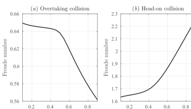
Figure 11.Froude number of mode-1 linear waves in the ISW-induced background shear current for(a)overtaking and(b)head-on collisions as a function of wavelength.
waves propagating to the right), we also examined head-on collisions. As shown in Fig. 10b, at the short-wave limit, the behaviour of the phase speed as a function of wavelength is very similar to that in the cases of an overtaking collision, ex-cept that now the phase speed is approaching the minimum current induced by the ISW.
We would like to note that given the nonlinear nature of the ISW, the interaction is indeed a nonlinear process, and thus the linear theory can only provide some rough guide for the flow behaviour. To measure the nonlinearity of the fluid flows, we shall introduce the Froude number which, in the context of internal wave dynamics, is usually defined as
Fr=U
c, (15)
whereU is the background current andcis the phase speed of the linear waves. The flow is said to be critical ifFr=1, in which case the nonlinear effects are dominant. In our sim-ulations, for anyx the vertically integratedU is essentially 0 since the flow is non-divergent in the simulation domain. Thus, a better estimation ofU would be the effective hori-zontal velocity in a reference frame moving with the ISW, which is essentially−cisw. In this reference frame, the
esti-matedcwould be−cisw+cpwherecp>0 for an overtaking
collision andcp<0 for a head-on collision. Hence, we can
define the Froude number in a reference frame moving with the ISW as
Fr= cisw cisw−cp
0 5 10 15 20 25 30 35 40 Wave number (m−1)
0 10 20 30
PS
D
O2 O3 O4 O6
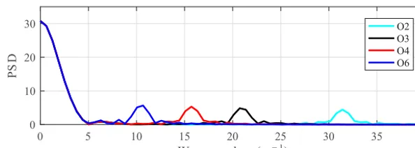
Figure 12.Power spectral density (PSD) of the initial horizontal velocity fields, computed from some of the overtaking collision cases.
Figure 11 shows the Froude number of the linear waves in the ISW-induced background current as a function of wave-length. The figure shows that Fr<1 for an overtaking col-lision andFr>1 for a head-on collision. In both cases,Fr approaches 1 at the short-wave limit since short waves prop-agate slower. This implies that in the interaction of ISWs with short waves, the nonlinear effects become more important as the wavelength of short waves becomes smaller.
5 Energetics
5.1 Diagnostic tool: power spectral density
A function that describes a physical process can be repre-sented either in the physical space or in the Fourier space. The two different representations are connected through the Fourier transform. Suppose f is a function of position x in the physical space, then the corresponding Fourier trans-formed variableF is a function of the horizontal wave num-berkand is given by
F (k)= ∞ Z
−∞
f (x)eikxdx. (17)
Ifxis bounded, thenktakes discrete values k=kn=
2nπ Lx
, n=0,1, . . .,∞. (18)
Parseval’s theorem states that the total power in a signal is the same whether it is computed in the physical space or in the Fourier space (Press et al., 2002). That is,
Total Power = Lx Z
0
|f (x)|2dx= ∞ X
n=0
|F (kn)|2dk. (19)
From this theorem, we can define the power spectral density (PSD) of the functionf as
PSD = |F (k)|2. (20)
The PSD is a function of the wave numberk. It can be inter-preted as the strength of the signal at each wave number. For this reason, it provides a powerful tool for analyzing physical processes.
5 10 15 20 25 30 35 40 0
0.2 0.4 0.6 0.8 1
O2 (t = 110 s) O2.5 (t = 113 s) O3 (t = 117 s) O4 (t = 126 s) O5 (t = 136 s) O6 (t = 146 s)
5 10 15 20 25 30 35 40
0 0.2 0.4 0.6 0.8 1
H2 (t = 84 s) H2.5 (t = 82 s) H3 (t = 80 s) H4 (t = 76 s) H5 (t = 73 s) H6 (t = 70 s)
Figure 13.Scaled PSD of linear waves in the simulations with(a)an overtaking collision and(b)a head-on collision atT =1.
0.2 0.25 0.3 0.35 0.4 0.45 0.5 0.55 0.6
0 0.5 1
Overtaking collision Head-on collision
Figure 14.Maximum values of the scaled PSD observed in Fig. 13 vs. their corresponding wavelengths.
5.2 Reduction of wave energy
In Fig. 13 we examine the energy reduction of linear waves due to collision by plotting the PSD of horizontal velocity in the wave number domain. The figure shows that in all cases, there is a net loss of wave energy due to the collision. It also shows that for a given solitary wave, the wavelength of the linear waves (which remains unchanged after the collision) is the single most important factor that determines the amount of PSD (and hence wave energy) remaining after the colli-sion. While the longest waves may retain as much as 85 % of the kinetic energy they had initially, the shortest waves lose almost all of their initial energy such that the peaks of the PSD can hardly be distinguished from background noise. Among other factors, a head-on collision is slightly more ef-ficient in destroying the linear waves than an overtaking col-lision, except for the small wavelength limit. This may be ex-plained by the fact that during a head-on collision, the struc-ture function (especially its peak) shifts further away from
its initial state than during an overtaking collision, as shown in Fig. 7, such that the new ISW-induced background envi-ronment is more difficult for the linear waves to adjust to. In contrast, the initial amplitude of the linear waves has very little impact on the net energy transfer due to collision, since curves produced from simulations in which the linear waves have an amplitude of 2 cm (not shown) are almost exactly the same as their smaller amplitude counterparts shown in Fig. 13a; though we did not consider large-amplitude short waves, since these will have their own complex dynamics.
Table 3.Quantitative measurement of the maximum values plotted in Fig. 14.
Wavelength Simulation and scaled PSD
Overtaking collision Head-on collision
0.2 m O2 9.08 % H2 13.69 %
0.25 m O2.5 15.69 % H2.5 16.43 %
0.3 m O3 30.39 % H3 20.52 %
0.4 m O4 48.14 % H4 38.17 %
0.5 m O5 77.76 % H5 57.54 %
0.6 m O6 85.11 % H6 68.18 %
Table 4.Quantitative measurement of the peak values observed in Fig. 15.
Simulation T =1 T =2 T =3 T=4
O6 85.11 % 76.08 % 66.40 % 60.20 %
H6 68.18 % 46.03 % 39.64 % 33.61 %
PSD atT =1 are at the level of 90 % but are never larger than 100 %, implying that very little wave energy is being trans-ferred from the short waves during the collision and that no energy is transferred from the ISW to the short waves. For the longest waves, the slight decrease in PSD is at a similar level to viscous dissipation. We note that this observation is con-sistent with the result shown in Fig. 10, since above the criti-cal wavelengthλ=0.5 m, very little energy exchange occurs due to the interaction.
For the cases O6 and H6, simulations were performed for an extended period of time in order to allow for repeated col-lisions between the solitary wave and the linear wave packet. For each of these cases, four complete collision cycles were observed, and the scaled PSD has been computed atT =1, 2, 3, and 4, as shown in Fig. 15. The corresponding measure-ment of the scaled PSD at each peak is given in Table 4. The figure and table suggest that for both cases, the scaled PSD is reduced after each subsequent collision, down to 60.20 % in the case of O6 and 33.61 % in the case of H6 atT =4. Nevertheless, they are still larger than those of the shorter waves after only one collision, implying that the wavelength is an important factor that determines the wave energy being transferred. Figure 15 and Table 4 also show that after each collision cycle, the scaled PSD in the case of H6 is always less than that of the case of O6, implying again that a head-on collisihead-on is more efficient in destroying the linear waves. 5.3 Influence of the interaction on the ISW
During the collision with the linear wave packet, the solitary wave is also affected by the linear waves that pass through it. We note, however, that the kinetic energy carried by the linear waves is much smaller than that carried by the solitary wave, and hence the impact of linear waves on the solitary
wave is also small. Here, we define the kinetic energy (KE) per unit mass following standard convention (which drops the reference density and hence changes the dimensions of the quantity) by
KE =1 2(u
2+w2). (21)
We found that when measured in terms of vertically inte-grated kinetic energy at the wave crest, the linear waves are about 1 % as energetic as the solitary wave.
To analyze changes in the solitary wave and determine if they are results of the collision, we performed an additional simulation with the same solitary wave but without the linear waves. We estimated the vertically integrated KE at the crest of the ISW for simulations with and without linear waves, and plotted the difference as time series (i.e. as functions of scaled timeT) in Fig. 16 over one complete collision cycle. Mathematically, this quantity is computed as
1 A0≤maxx≤Lx
Lz Z
0
(KEfull − KEisw)dz
, (22)
whereAis the normalization factor defined as the maximum vertically integrated KE of the initial solitary wave. The sub-script “full” denotes variables from simulations with both solitary and linear waves, and the subscript “isw” denotes variables from simulations with a freely propagating solitary wave. For linear waves with a wavelengthλ=0.2 m shown in Fig. 16a, there is a net energy transfer into the solitary wave as a result of the interaction, such that the maximum vertically integrated KE has increased by at least 1 %. We are able to confirm that such an energy increase in the soli-tary wave is robust since we have also performed additional simulations with a longer linear wave packet (not shown), and found that the maximum vertically integrated KE in-creases approximately linearly with respect to the length of the wave packet. On the other hand, for waves with a wave-lengthλ=0.6 m shown in Fig. 16b, energy increase in the solitary waves after the collision is insignificant. In all cases, the curves shown demonstrate periodicity associated with their particular wavelengths.
We have also attempted to detect the phase shift of the solitary waves from the locations of maximum vertically in-tegrated KE. However, we found that such a phase shift, if it exists at all, is on the order of millimetres. In other words, the detected phase shift is on the grid scale and is subject to numerical error. For this reason, the results are not shown here.
6 Conclusions
8 10 12 14 16 18 20 0
0.2 0.4 0.6 0.8 1
T = 1 (t = 146 s) T = 2 (t = 292 s) T = 3 (t = 438 s) T = 4 (t = 584 s)
8 10 12 14 16 18 20
0 0.2 0.4 0.6 0.8 1
T = 1 (t = 70 s) T = 2 (t = 140 s) T = 3 (t = 210 s) T = 4 (t = 280 s)
Figure 15.Scaled PSD of the cases(a)O6 and(b)H6 after repeated collisions.
-0.01 0 0.01 0.02 0.03
Scaled
KE
(a ) Wavelength = 0.2 m
O2 H2
0 0.1 0.2 0.3 0.4 0.5 0.6 0.7 0.8 0.9 1
T
-0.1 0 0.1
Scaled
KE
(b) Wavelength = 0.6 m
O6 H6
Figure 16.Time series of scaled maximum vertically integrated kinetic energy (KE). The figure shows the difference between simulations with and without the linear waves. Note the different scales in theyaxes.
fully nonlinear ISW and small-scale linear internal waves. We demonstrated that there was a net energy transfer from the small-scale linear waves to the large-scale solitary waves. This contrasts the conclusion in Broutman and Young (1986), made for a different type of internal wave interaction, that energy is transferred from large-scale waves to small-scale waves. Our simulation results suggest that during the inter-action, the solitary wave essentially acts as a filter through which only long waves may pass. For waves with a smaller wavelength, the interaction leads to a reduction of their initial energy and a destruction of their spatial structure. These pro-cesses occur in a background state set by the solitary-wave-induced stratification and current. During the interaction,
ad-justment of the short waves to this new background environ-ment extracts their wave energy and modifies the wave struc-ture. The fact that short waves may not survive the interac-tion with a solitary wave, or more generally any localized nonlinear background environment which both deforms the pycnocline and induces shear, implies that the observed spec-trum of wavelengths of internal waves in locations with large amplitude ISWs (such as Straits) is likely to be deficient in short waves. At the time of writing we are unaware of mea-surements to support or contradict this hypothesis.
the presence of ISW-induced velocity shear, which alters the vertical structure of the short waves in a nonlinear manner, leading to significant wave amplitudes on only one side of the deformed pycnocline centre. On the other hand, a shift of the location of the pycnocline plays a secondary role dur-ing the collision, as its main effect is to alter the propagation speed of the linear waves, and shift the location of the maxi-mum of the vertical structure downward. However, the verti-cal structure is unchanged with respect to the pycnocline cen-tre. We also demonstrated that a critical layer is not present during the collision, regardless of the wavelength of the lin-ear waves, since the phase speed approaches the maximum ISW-induced current asymptotically as the wavelength ap-proaches 0.
A clear avenue of future research is to explore the param-eter space, in particular the Richardson number effect, of the solitary wave. In the present work, we studied the ISW whose minimum Richardson number is 0.246. Although none of the simulations show evidence of the generation of shear insta-bility, this does not necessarily mean that the wave–wave interaction considered in the present work is Richardson number independent. Moreover, Lamb and Farmer (2011) showed that it is not only the minimum Richardson number but also the length of the unstable region with a low Richard-son number relative to the wavelength of ISW that is jointly responsible for the generation of shear instability in an ISW. It is thus reasonable to assume that the relative length of the region with a low Richardson number in the ISW also has an influence on the wave–wave interaction. Future research will explore these effects in detail.
We note that our findings are in many ways similar to those in Stastna et al. (2015). Their study also concluded that the direction of energy transfer during the interaction is from the small-scale weakly nonlinear wave (i.e. the mode-2 wave) to the large-scale solitary wave (i.e. the mode-1 wave), and that such energy transfer is more efficient when a head-on, instead of overtaking, collision is involved. The main differ-ence is that in a mode-1–mode-1 interaction, there is a cutoff determined by the wavelength of short waves, above which the small-scale waves maintain their structure after interac-tion, whereas a mo1–mo2 interaction is much less de-pendent on the wavelength. In a mode-1–mode-1 interac-tion, this cutoff corresponds to the wavelength at which the phase speed of the short waves upstream of the solitary wave exceeds the maximum ISW-induced current. In a mode-1– mode-2 interaction, however, this cutoff does not exist since the maximum ISW-induced current is always larger than the phase speed for any given wavelengths.
While all of the simulations discussed in this work are per-formed on the laboratory scale, the scaling-up of the current experiments to the field scale is left as a topic for future work. When the field scale is considered, waves with a much larger range of wavelengths can be expected to breakdown, in-cluding short waves affected by self-interaction (Sutherland, 2016). Also, a higher Reynolds number implies that the
turning seen in Fig. 6 may eventually lead to significant over-turns. The three-dimensionalization of the flow field should also be examined. As shown in Andreassen et al. (1994), two-dimensional models are unable to properly describe the physics or the consequences of the wave-breaking process, in particular those consequences induced by the presence of a critical layer. We also note that in two dimensions, the only possible form of wave–wave interaction is either an overtak-ing collision or a head-on collision. However, observational evidences (e.g. Quaresma et al., 2007; in particular, see their Figs. 2 and 8) suggest that internal waves do not generally propagate parallel to each other but may interact at different angles. The effects of directionality of wave propagation is another topic that can be considered in forthcoming studies.
Data availability. Data is available upon request by email to the first author.
Competing interests. The authors declare that they have no conflict of interest.
Special issue statement. This article is part of the special issue “Ex-treme internal wave events”. It is a result of the EGU, Vienna, Aus-tria, 23–28 April 2017.
Acknowledgements. Time-dependent simulations were completed on the high-performance computer cluster Shared Hierarchi-cal Academic Research Computing Network (SHARCNET, www.sharcnet.ca). Chengzhu Xu was supported by an Ontario Graduate Scholarship while Marek Stastna was supported by an NSERC Discovery Grant RGPIN-311844-37157.
Edited by: Kateryna Terletska Reviewed by: two anonymous referees
References
Andreassen, Ø., Wasberg, C. E., Fritts, D. C., and Isler, J. R.: Grav-ity wave breaking in two and three dimensions: 1. Model descrip-tion and comparison of two-dimensional evoludescrip-tions, J. Geophys. Res.-Atmos., 99, 8095–8108, 1994.
Broutman, D. and Young, W. R.: On the interaction of small-scale oceanic internal waves with near-inertial waves, J. Fluid Mech., 166, 341–358, 1986.
Cai, S., Long, X., Dong, D., and Wang, S.: Background current af-fects the internal wave structure of the northern South China Sea, Prog. Nat. Sci., 18, 585–589, 2008.
Dunphy, M. and Lamb, K. G.: Focusing and vertical mode scatter-ing of the first mode internaltide by mesoscale eddy interaction, J. Geophys. Res.-Oceans, 119, 523–536, 2014.
double-humped solitary waves, Nonlin. Processes Geophys., 18, 351– 358, https://doi.org/10.5194/npg-18-351-2011, 2011.
Grisouard, N. and Thomas, L. N.: Critical and near-critical reflec-tions of near-inertial waves off the sea surface at ocean fronts, J. Fluid Mech., 765, 273–302, 2015.
Helfrich, K. R. and Melville, W. K.: Long nonlinear internal waves, Annu. Rev. Fluid Mech., 38, 395–425, 2006.
Klymak, J. M. and Moum, J. N.: Internal solitary waves of elevation advancing on a shoaling shelf, Geophys. Res. Lett., 30, 2045, https://doi.org/10.1029/2003GL017706, 2003.
Kundu, P. K., Cohen, I. M., and Dowling, D. R.: Fluid Mechanics, 5th edn., Academic Press, Waltham, MA, USA, 2012.
Lamb, K. G.: Are solitary internal waves solitons?, Stud. Appl. Math., 101, 289–308, 1998.
Lamb, K. G.: Theoretical descriptions of shallow-water solitary internal waves: comparisons with fully nonlinear waves, in: The 1998 WHOI/IOS/ONR Internal Solitary Wave Workshop: Contributed Papers, October 1998, Sydney, British Columbia, Canada, 209–217, 1999.
Lamb, K. G.: A numerical investigation of solitary internal waves with trapped cores formed via shoaling, J. Fluid Mech., 451, 109–144, 2002.
Lamb, K. G.: Shoaling solitary internal waves: on a criterion for the formation of waves with trapped cores, J. Fluid Mech., 478, 81–100, 2003.
Lamb, K. G.: Extreme internal solitary waves in the ocean: the-oretical considerations, in: Proceedings of the 14th ’Aha Hu-liko’a Hawaiian Winter Workshop, 25–28 January 2005, Hon-olulu, Hawaii, USA, 109–117, 2005.
Lamb, K. G. and Farmer, D.: Instabilities in an internal solitary-like wave on the Oregon Shelf, J. Phys. Oceanogr., 41, 67–87, 2011. Lamb, K. G. and Yan, L.: The evolution of internal waves undular bores: comparisons of a fully nonlinear numerical model with weakly nonlinear theory, J. Phys. Oceanogr., 26, 2712–2734, 1996.
Press, W. H., Teukolsky, S. A., Vetterling, W. T., and Flannery, B. P.: Numerical Recipes in C, Cambridge University Press, 2nd edn., Cambridge, UK, 2002.
Quaresma, L. S., Vitorino, J., Oliveira, A., and da Silva, J.: Evi-dence of sediment resuspension by nonlinear internal waves on the western Portuguese mid-shelf, Mar. Geol., 246, 123–143, 2007.
Sarkar, S. and Scotti, A.: From topographic internal gravity waves to turbulence, Annu. Rev. Fluid Mech., 49, 195–220, 2017. Scotti, A. and Pineda, J.: Observation of very large and steep
inter-nal waves of elevation near the Massachusetts coast, Geophys. Res. Lett., 31, L22307, https://doi.org/10.1029/2004GL021052, 2004.
Stastna, M. and Lamb, K. G.: Large fully nonlinear internal solitary waves: the effect of background current, Phys. Fluids, 14, 2987– 2999, 2002.
Stastna, M., Olsthoorn, J., Baglaenko, A., and Coutino, A.: Strong mode-mode interactions in internal solitary-like waves, Phys. Fluids, 27, 046604, https://doi.org/10.1063/1.4919115, 2015. Subich, C. J., Lamb, K. G., and Stastna, M.: Simulation of the
Navier–Stokes equations in the three dimensions with a spectral collocation method, Int. J. Numer. Mech. Fl., 73, 103–129, 2013. Sun, O. and Pinkel, R.: Energy transfer from high-shear, low-frequency internal waves to high-low-frequency waves near Kaena Ridge, Hawaii, J. Phys. Oceanogr., 42, 1524–1547, 2012. Sutherland, B. R.: Excitation of superharmonics by internal modes
in non-uniformly stratified fluid, J. Fluid Mech., 793, 335–352, 2016.
Thorpe, S. A.: The Turbulent Ocean, Cambridge University Press, Cambridge, UK, 2005.
Trefethen, L. N.: Spectral Methods in Matlab, Society for Industrial and Applied Mathematics, Philadelphia, PA, USA, 2000. Turkington, B., Eydeland, A., and Wang, S.: A computational