www.clim-past.net/8/117/2012/ doi:10.5194/cp-8-117-2012
© Author(s) 2012. CC Attribution 3.0 License.
Climate
of the Past
Climate variability in Andalusia (southern Spain) during the period
1701–1850 based on documentary sources: evaluation and
comparison with climate model simulations
F. S. Rodrigo1, J. J. G´omez-Navarro2, and J. P. Mont´avez G´omez2
1Departamento de F´ısica Aplicada, Universidad de Almer´ıa, La Ca˜nada de San Urbano, s/n, 04120, Almer´ıa, Spain 2Grupo de Modelizaci´on Atmosf´erica Regional, Departamento de F´ısica, Universidad de Murcia, Spain
Correspondence to: F. S. Rodrigo ([email protected])
Received: 17 June 2011 – Published in Clim. Past Discuss.: 7 July 2011
Revised: 23 November 2011 – Accepted: 24 November 2011 – Published: 10 January 2012
Abstract. In this work, a reconstruction of climatic condi-tions in Andalusia (southern Iberian Peninsula) during the period 1701–1850, as well as an evaluation of its associated uncertainties, is presented. This period is interesting because it is characterized by a minimum in solar irradiance (Dal-ton Minimum, around 1800), as well as intense volcanic ac-tivity (for instance, the eruption of Tambora in 1815), at a time when any increase in atmospheric CO2concentrations
was of minor importance. The reconstruction is based on the analysis of a wide variety of documentary data. The re-construction methodology is based on counting the number of extreme events in the past, and inferring mean value and standard deviation using the assumption of normal distribu-tion for the seasonal means of climate variables. This recon-struction methodology is tested within the pseudoreality of a high-resolution paleoclimate simulation performed with the regional climate model MM5 coupled to the global model ECHO-G. The results show that the reconstructions are in-fluenced by the reference period chosen and the threshold values used to define extreme values. This creates uncertain-ties which are assessed within the context of climate simu-lation. An ensemble of reconstructions was obtained using two different reference periods (1885–1915 and 1960–1990) and two pairs of percentiles as threshold values (10–90 and 25–75). The results correspond to winter temperature, and winter, spring and autumn rainfall, and they are compared with simulations of the climate model for the considered period. The mean value of winter temperature for the pe-riod 1781–1850 was 10.6±0.1◦C (11.0◦C for the reference period 1960–1990). The mean value of winter rainfall for the period 1701–1850 was 267±18 mm (224 mm for 1960–
1990). The mean values of spring and autumn rainfall were 164±11 and 194±16 mm (129 and 162 mm for 1960–1990, respectively). Comparison of the distribution functions cor-responding to 1790–1820 and 1960–1990 indicates that dur-ing the Dalton Minimum the frequency of dry and warm (wet and cold) winters was lower (higher) than during the refer-ence period: temperatures were up to 0.5◦C lower than the 1960–1990 value, and rainfall was 4 % higher.
1 Introduction
Anthropogenic influences on climate overlie a background of natural climate variability that may diminish or increase the same (IPCC, 2007). The lack of instrumental surface temperature and precipitation records prior to the mid-19th century underlines the need to reconstruct the history of cli-mate changes from proxies of clicli-mate variability derived from the environment itself and from documentary sources (Rutherford et al., 2005).
31 2
3 4 5 6 7 8 9 10 11 12 13 14 15 16 17 18 19 20 21 22 23 24 25 26
Figure 1 27
*Hu
*Ma *Ca
*Se
*Gi
*Al *Co
*Gr *Ja
38ºN 40ºN 42ºN
8ºW 6ºW 4ºW 2ºW 0º 2ºE
100 km
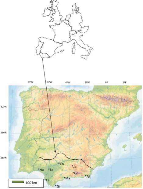
Fig. 1. Map of the study region. Main cities with instrumental and documentary data are indicated (code in Table 1).
Portugal (Alcoforado et al., 2000; Taborda et al., 2004), and Castile, a central region in Spain (Rodrigo et al., 1998; Bull´on, 2008; Dom´ınguez-Castro et al., 2008). In addition, various studies coordinating data for the entire Iberian Penin-sula have been published, related to flood events in Spanish river basins since 1500 AD (Barriendos and Rodrigo, 2006), droughts during the 17th century and the first half of the 18th century (Dom´ınguez-Castro et al., 2010), and seasonal and annual rainfall variability from the 16th to 20th centuries (Rodrigo and Barriendos, 2008).
The climate of Andalusia (southern Spain, Fig. 1) is Mediterranean, but with a strong influence of the Atlantic Ocean, mainly to the west of the region. The latitude (around 37◦N), midway between the temperate oceanic climate zone to the north and the warm tropical one to the south, pro-duces atmospheric behavior of transition between two cli-mates. Its geographical position (southwestern Europe) ex-poses it to the typical influences of the planetary temperate zone of middle latitudes, as well as certain tropical influences (Mart´ın-Vide, 2007). Therefore, the study of this region is of great interest.
Previous historical climatology studies in this region have analyzed the annual (Rodrigo et al., 2000) and winter (Ro-drigo, 2008) rainfall variability since the 16th century. In
historical climatology it is always possible to find new docu-mentary data that compel us to revise analysis. Therefore, the main objective of this work is to improve the reconstructions of the past Andalusian climate, adding new records cover-ing the period from 1701 to 1850, especially from 1780 on-wards. This period includes the Dalton Minimum (Wagner and Zorita, 2005) between approximately 1790 and 1830, a period characterized by a minimum in solar irradiance and intense volcanic activity, with the Tambora eruption in April 1815 as main event (Trigo et al.,2009). From a climatic point of view, therefore, the analysis of climatic data during this period is particularly interesting due to the role of these external forcing factors (Wagner and Zorita, 2005; Trigo et al., 2009). An additional source of information on past cli-mate variability is provided by clicli-mate model simulations. The analysis of model responses to external forcing, changes in atmosphere and ocean mechanisms contributing to natu-ral climate variability as well of comparisons between model and proxy data help to improve our understanding of past climate variability (Br´azdil et al., 2011). Therefore, other important objectives of this work are an evaluation of the re-construction method using climate model simulations, and a comparison of climate reconstructions with climate model simulations.
The paper is organized in the following way: data are pre-sented in Sect. 2 (a list of new documentary sources is in-cluded in Appendix A), and the reconstruction methodol-ogy used is explained in Sect. 3. Section 4 presents the main results, in Sect. 5 these results are compared with other data, and conclusions and challenges for future research are presented in Sect. 6.
2 Data
2.1 Documentary data
previous works (Rodrigo et al., 1999; Rodrigo, 2008) have been enlarged, adding new data sources recently discovered, basically early newspapers and medical studies. From the late years of the 18th century to the first decades of the 19th century, anonymous observers began to send their meteoro-logical observations to local newspapers to ensure that peo-ple were informed of them. Instrumental daily meteorolog-ical data appear in most of them. Although their spatio-temporal coverage is incomplete, these data sources may complete the description of general climatic conditions as well as the nature and character of extreme events in the past. Empirical research of a medical and geographical nature be-gan in Spain in the 18th century with a set of studies that considered the strong influence of climate and environment on the appearance of illness and epidemics. These studies are called “medical topographies”, and on many occasions, they included meteorological observations made by physicians. A summary of the new data sources used in this work is shown in Appendix A.
The compiled reports were first codified. This allowed the ordering of information into time-space and type (rain, thermal, wind, cloudiness). Most data relate to Seville and the Guadalquivir River Basin (46.4 %), Granada together with Sierra Nevada Mountains (14.0 %), and Malaga on the Mediterranean coast (13.4 %). Most data correspond to rain-related phenomena (68 %), basically extreme events, such as continuous and intense rainfall, floods and droughts, but 15 % of the records are related with the thermal regime (heat and cold waves, frosts, snowfalls) and 17 % of the records related to other events, such as winds and fogs. In the case of temperatures, the subjective appraisals of the au-thors on the degree of cold or heat were only taken into account when they were associated with more objective ob-servations, such as those related to frosts, snowfalls, thun-derstorms, etc, or when they referred to unusually extreme weather. News related with frosts, snowfalls, or excessive cold unusual for the season (spring, summer) were consid-ered as cold extremes. News related with heat in months when it is not usual (between November and February), or convective storms between the end of spring and the begin-ning of the autumn (May to September) were considered as warm extremes, since these phenomena are related with the relative low-pressure presence of thermal origin in the IP. Time resolution depends on the data source, varying from daily (57.6 %) to annual (7 %). For the purposes of this study, a seasonal resolution was chosen, considering the sea-sons of the year in the usual way, that is, winter = December to February, spring = March to May, summer = June to Au-gust, and autumn = September to November. The informa-tion varies seasonally, with 36.6 % of the news referring to winter, 25.4 % to autumn, 22.9 % to spring, and 15.1 % to summer. This distribution is a result of the interest of data sources affecting the state of agriculture and the evolution of crops, especially wheat sown in autumn and harvested in early June. 32 1 2 3 Figure 2 4 5 6 7 8 9 10 11 0 10 20 30 40 50
1700 1720 1740 1760 1780 1800 1820 1840 1860
N
(a) Records per year
0 25 50 75 100 125 150
1700 1720 1740 1760 1780 1800 1820 1840 1860
N
(b) Records per decade
32 1 2 3 Figure 2 4 5 6 7 8 9 10 11 0 10 20 30 40 50
1700 1720 1740 1760 1780 1800 1820 1840 1860
N
(a) Records per year
0 25 50 75 100 125 150
1700 1720 1740 1760 1780 1800 1820 1840 1860
N
(b) Records per decade
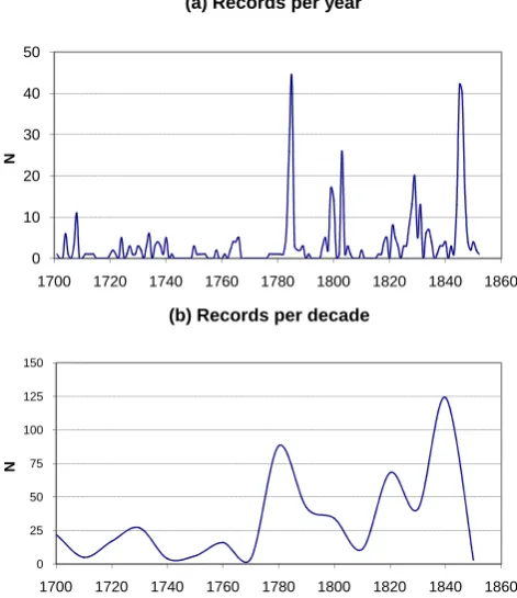
Fig. 2. Number of records from documentary sources, (a) by year, (b) by decade, during the period 1701–1850.
Documentary data refer to the period 1701–1850 (from 1851 onwards available instrumental data were at least with monthly resolution). For the entire period from 1701 to 1850, the average number of records is 3.4 items yr−1, an informa-tion density higher than that from previous studies for this region (2.6 items yr−1, see Rodrigo et al., 1999). The time coverage of these data is shown in Fig. 2, which shows the number of records per year and decade. It may be seen that the density of information increases notably from 1780s on-wards, with peaks around the first decades of the 1800s. In a preliminary view, these peaks correspond to a highest fre-quency of extreme events, with winter as the season of the year with most records.
Table 1. Meteorological stations in Andalusia (height expressed in meters above sea level; PeriodT= period of daily instrumental
observa-tions of temperature; PeriodR: idem for monthly rainfall).
Station (Code) Longitude Latitude Height PeriodT PeriodR
Almeria (Al) 01◦230W 36◦510N 20 1908–2005
Cadiz (Ca) 06◦200W 36◦450N 12 1851–2005 1821–2005
Cordoba (Co) 04◦510W 37◦510N 92 1894–2005
Gibraltar (Gi) 05◦210W 36◦080N 8 1813–2005
Granada (Gr) 03◦370W 37◦080N 685 1893–2005 1898–2005
Huelva (Hu) 06◦560W 37◦150N 26 1903–2005 1903–2005
Jaen (Ja) 03◦480W 37◦480N 484 1867–2005
Malaga (Ma) 04◦290W 36◦400N 7 1893–2005 1878–2005
Seville (Se) 05◦530W 37◦250N 31 1893–2005 1865–2005
focus on tail behavior of the distribution function and thresh-old values low enough to ensure that a reasonable number of exceedances occur (Solow, 1999). If the threshold val-ues are the percentiles 10 and 90 (c10 andc90, respectively),
π= Prob{X < c10}+ Prob{X > c90}= 0.20. These percentiles
are commonly used to define the frequency of extreme in-dices, such as cold nights or warm days, and correspond to moderately extreme events (Zhang et al., 2005). The ex-pected valuehniand variance var(n) of the distribution for
m=31 are hni =π m=6.2, and var(n) =mπ(1-π )=4.96, respectively. Similar to Briffa et al. (2002) or Pauling et al. (2006), we use±2 SE to provide an estimate of the uncer-tainties that are associated with the estimation of the number of extreme seasons. Therefore, we will consider that the to-tal number of extreme seasons is satisfactory when it is in-cluded in the intervalhni±2√var(n) = (1.7, 10.6). The av-erage number of extreme seasons in the case of winter tem-peratures (since 1780) is 4.3 extreme seasons for each 31-yr period. Mean values of the other seasons of the year are 1.3 for spring, and 1.1 for summer and autumn. In the case of rainfall, the average number of extreme seasons for each 31-yr period are 7.6, 7.4, 4.2, and 7.2 for, respectively, winter, spring, summer, and autumn. As a consequence, in the fol-lowing we will focus our study on winter temperature and seasonal rainfall, and cases of spring, summer, and autumn temperatures will not be considered.
2.2 Instrumental data
Instrumental regional series of seasonal temperature and pre-cipitation were obtained from the 19th century to 2005, us-ing the longest available data series in Andalusia (five sta-tions for temperature, since 1851, and nine stasta-tions for rain-fall, since 1813, see Table 1). These series, in general terms, coincide with the locations of the documentary data in the pre-instrumental period. All the stations are distributed around 36–37◦N latitude, and between 1◦and 7◦W longi-tude, with different heights above sea level (from M´alaga at 7 m a.s.l. to Granada at 685 m a.s.l.). Temperature series
are from the SDATS database (Spanish Daily Temperature Data, Brunet et al., 2006) and rainfall series were provided by the Spanish Meteorological Agency (http://www.aemet.es) and the British Meteorological Office in the case of Gibral-tar (Wheeler, 2007). All of them are high quality series, without homogeneity problems (Almarza et al., 1996). Lo-cal monthly rainfall totals were used to obtain seasonal total rainfall. The regional series was obtained for each season by averaging the corresponding local values, and consider-ing in each year the number of stations with data. This pro-cedure was followed because a common period would be too short (since 1903 for temperatures and 1908 for rain-fall), removing from the instrumental series the period 1885– 1915, which was considered as reference period (see below). This procedure does not substantially bias the results. Ta-ble 2 shows the statistics corresponding to the reference pe-riod 1960–1990. The construction of a regional series is justified by the analysis of the spatio-temporal variability in the region. The application of empirical orthogonal func-tion (EOF) analysis to Andalusian stafunc-tions during the period 1867–2003 (Castro-D´ıez et al.,2007) showed that, at sea-sonal and annual timescales, the first leading EOF pattern (explaining more than 50 % of the variance for both, tem-perature and precipitation) presents high correlations with all the stations, particularly in winter (65.69 % of explained variance for precipitation, 72.56 % for temperature). Basic statistics correspond to Mediterranean climatic characteris-tics, with wet and mild winters, warm and dry summers, and spring and autumn as transition seasons. A season may be characterized as dry (cold) if total rainfall (average tempera-ture) is lower than the 10th or 25th percentile of the reference period (c10 andc25, respectively). Similarly, a season was
considered as wet (warm) if total rainfall (average tempera-ture) was higher than the 75th or 90th percentile of the ref-erence period (c75 andc90, respectively). These percentiles
Table 2. Main statistics of the seasonal regional series for
tem-perature (T in◦C) and precipitation (R in mm) for the reference
period 1960–1990 (u= mean value;s= standard deviation;ci= i-th
percentile; KS = Kolmogorov-Smirnov statistic, in bold if the hy-pothesis of conforming to a normal distribution is not rejected at
the 95 % confidence level KS<0.161 forN=30 (Wilks, 1995).
Parameter Winter Spring Summer Autumn
u(T ) 11.0 15.5 23.9 18.5
s(T ) 0.8 0.8 0.7 1.0
c10(T ) 10.0 14.6 23.1 17.3
c25(T ) 10.4 15.0 23.7 17.8
c75(T ) 11.6 16.1 24.3 18.9
c90(T ) 12.0 16.6 24.6 19.8
KS(T) 0.078 0.088 0.149 0.106
u(R) 224.2 128.8 22.8 162.3
s(R) 111.1 56.8 12.3 86.4
c10(R) 111.0 70.4 10.3 56.9
c25(R) 147.1 87.1 14.1 87.0
c75(R) 271.1 155.3 24.9 212.7
c90(R) 381.5 197.0 37.6 263.5
KS(R) 0.124 0.118 0.182 0.106
was applied to test the normality of the distribution. It was seen that there is not enough evidence to prove that the dis-tribution is not normal, at a 95 % confidence level, except in the case of summer rainfall.
2.3 Simulated climate in Andalusia
A climate simulation was used to test some aspects of the methodology and to evaluate the magnitude of the uncertain-ties of the methodology, as further discussed in the next sec-tion. The simulation covers the IP with a spatial resolution of 30 km during the period 1001–1990. It was performed with a climate version of the regional model MM5, and was driven through the domain boundaries by a simulation performed with the Global Circulation Model ECHO-G (Zorita et al., 2005). Both simulations consider variations in three main external factors: concentration of greenhouse gases, total so-lar irradiance at the top of the atmosphere, and the effect of large volcanic events. These factors behave in the simula-tion according to the reconstrucsimula-tion by Crowley (2000). This simulation has demonstrated to simulate realistically many aspects of the climate of the IP in the recent past, where there are reliable data and observations to compare with, and significantly improves the accuracy of the simulation per-formed with the global model alone. The reader is referred to G´omez-Navarro et al. (2011) for a technical description and validation of this simulation. The present article focuses on the simulated seasonal means of temperature and rainfall regionally averaged over Andalusia.
3 Methodology
The reconstruction methodology used was explained in Rodrigo (2008). The basic ideas are the following:
Hypothesis 1: past extreme events may be defined in a sim-ilar way to present events; that is, we assume that threshold values of the reference period were exceeded when there was an extreme event in the past.
The starting point of the study consists of simply estimat-ing the frequency of extreme seasons in past periods. A season is considered extreme if documentary data provides information on the occurrence of extreme events during the corresponding months (heat waves, snowfalls, frosts, intense and/or continuous rainfall, floods, droughts). The length of the periods considered is 31 yr, which allows comparison with the modern reference period. In this way, the numbers nl
and nhof, respectively, dry or cold, and wet or warm seasons
within a given 31-yr period may be established.
If FX is the distribution function representative of the
climate variable (in our case, seasonal average tempera-ture and rainfall), the quantilesql andqhof the distribution
function, corresponding to dry/cold and wet/warm seasons, respectively, may be found as
nl
n =Prob{X≤ql} =FX(ql)→ql=F
−1
x (ql)
nh
n =Prob{X > qh} =Prob{X≤qh}
=1−FX(gh)→gh=FX−1
1−nh
n
(1) where n is the total number of seasons in the chosen period (in our case,n=31).
Hypothesis 2: the distribution function representative of the climatic variable is the standardized normal distribution of mean 0 and standard deviation 1, that isFX=N (0;1).
The normal distribution function is the simplest choice, bearing in mind that the regional series of temperature and precipitation are obtained as the average value of the individ-ual series. For the time scales at which we are working, the precipitation amounts tend to be more closely approximated as the normal distribution because of the central limit the-orem, which states that under fairly general conditions, the sum of independent variables approaches the normal distri-bution (Lettenmaier, 1995). This hypothesis, in the case of Andalusian rainfall, is valid for all the seasons of the year, except summer (Rodrigo, 2002), and it was tested for the in-strumental regional series of the reference period (Table 2).
The quantiles of the series may be established using c = u
+ sq, whereuis the mean value, s the standard deviation,
c the quantile of the non-standardized normal distribution
N(u,s), andqthe quantile of theN (0;1). Therefore,
cl= u+sqlch=u+sqh (2)
mean valueuand standard deviationsof a given period may be found as
u=ch– sqh=cl–sql. (3)
Summarizing, for each 31-yr period, from documentary data analysis, nland nhare calculated. These numbers are used to
estimateqlandqh, and thesanduvalues are estimated
con-sidering the values ofclandchcorresponding to the reference
period.
The advantages of this method are that it reduces possi-ble subjectivity propossi-blems (due to the documentary source, or the researcher) associated with the assignment of ordinal in-dices to quantify documentary data, and it does not need an overlapping period with instrumental data to obtain quantita-tive estimates of the climate variables in the past. Changes in the mean value and/or in the standard deviation will yield changes in the probability of extreme events, and, therefore, in the frequency of these events. Our aim is to study the in-verse problem, that is, infer changes in mean and standard deviation from the frequency of extreme events, keeping in mind that documentary data basically reflect the occurrence of extreme events and their impacts.
The application of this method is only possible if we have sufficient data to accomplish the different steps. In fact, if nl=0, then ql→ −∞, and if nh=0, then qh→
∞. Therefore, the absence of information on extremes in certain periods implies the appearance of gaps in the reconstructed series.
This methodology can be tested within the context of the pseudoreality of the climate simulation. The underlying idea is that even if the evolution of the simulation does not per-fectly match the real evolution of the climate in the past millennium, it represents a feasible evolution of the climate since it is physically self-consistent. Thus, the statistical properties of the simulated variables, and their physical re-lationships, are a reliable version of the actual ones. An ob-vious advantage of using a climate model is that within the simulation the information is available at all temporal and spatial scales. Thus, one can construct a pseudoproxy in-side the model for a given variable, apply the reconstruction methodology to be tested and generate a pseudoreconstruc-tion. This can be later compared with the simulated evolution of the variable, which is known. It is important to note that this exercise does not validate the model, but the methodol-ogy used to reconstruct the actual climate.
The procedure to create the pseudoproxy is as follows. A reference period has to be chosen, as well as a probability threshold, to define what an extreme event is. Once this is fixed, thechandcl values can be found. The next step is to
compare the simulated seasonal means with these percentiles to obtain a series of 0s and 1s representing the occurrence or not of an extreme season. Using a running window of 31 yr, the number of extreme seasons in a given period,nlandnh,
can be estimated, which are the pseudoproxy.
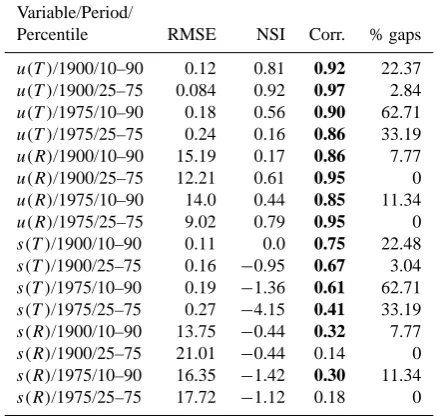
Table 3. Statistics of the reconstruction method when applied to all the simulated series of mean value (u) and standard deviation (s)
of winter temperature (T, in◦C) and rainfall (R, in mm) shown in
Figs. 3 and 4. Shown are the Root Mean Square Error (RMSE), the Nash-Sutcliffe index (NSI), the correlation (Corr) and the per-centage of gaps (% gaps) in the reconstruction. Bold numbers in correlation denotes statistically significant at the 95 % confidence level.
Variable/Period/
Percentile RMSE NSI Corr. % gaps
u(T )/1900/10–90 0.12 0.81 0.92 22.37
u(T )/1900/25–75 0.084 0.92 0.97 2.84
u(T )/1975/10–90 0.18 0.56 0.90 62.71
u(T )/1975/25–75 0.24 0.16 0.86 33.19
u(R)/1900/10–90 15.19 0.17 0.86 7.77
u(R)/1900/25–75 12.21 0.61 0.95 0
u(R)/1975/10–90 14.0 0.44 0.85 11.34
u(R)/1975/25–75 9.02 0.79 0.95 0
s(T )/1900/10–90 0.11 0.0 0.75 22.48
s(T )/1900/25–75 0.16 −0.95 0.67 3.04
s(T )/1975/10–90 0.19 −1.36 0.61 62.71
s(T )/1975/25–75 0.27 −4.15 0.41 33.19
s(R)/1900/10–90 13.75 −0.44 0.32 7.77
s(R)/1900/25–75 21.01 −0.44 0.14 0
s(R)/1975/10–90 16.35 −1.42 0.30 11.34
s(R)/1975/25–75 17.72 −1.12 0.18 0
An important drawback of applying the above methodol-ogy is that a reference period, as well as a probability thresh-old to define an event extreme, has to be arbitrarily defined. The reconstruction methodology is in principle sensitive to this choice, introducing an uncertainty factor which is impor-tant to assess. Four different combinations have been tested in the present study: two reference periods (the 31-year peri-ods 1885–1915 and 1960–1990) with two pairs of probability thresholds (percentiles 10–90 and 25–75), receptively. The period 1885–1915 was chosen because a priori it is markedly different from the modern period 1960–1990, and it is ex-pected that the effects of global warming would have been of less importance during these years (it is a transition period between the end of the Little Ice Age and the modern warm-ing period). This exercise was applied to the simulated win-ter mean series of temperature and precipitation (the results for other seasons are similar, and are not shown) to recon-struct the simulated evolution of these variables during the last millennium.
7 7.5 8 8.5 9 9.5
7 7.5 8 8.5 9
80 100 120 140 160 180 200 220
80 100 120 140 160 180 200 220
1000 1200 1400 1600 1800 2000
u(T)
(ºC
)
u(R)
(m
m)
ref. 1900
ref. 1900 ref. 1975
ref. 1975
year
perc. 10-90 perc. 25-75 simulation
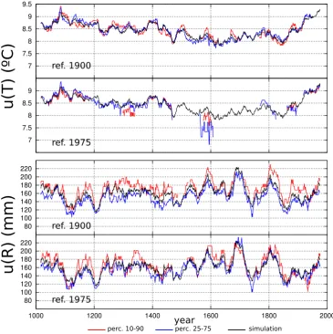
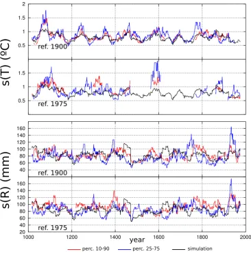
Fig. 3. Evolution (in black) of the 31-yr running mean of temperature (two upper panels) and precipitation (two lower panels) in the climate simulation for the last millennium. Four pseudoreconstructions are shown, using the periods 1885–1925 (first and third panels) and 1960– 1990 (second and fourth panels) using the 10–90 (red lines) and 25–75 (blue lines) percentiles.
and 25–75, in red and blue, respectively). Overall, there is a good agreement between the original and reconstructed se-ries, although it is slightly better when the larger percentiles are used. This is a statistical problem linked to the ability of a set of only 31 elements to sample the tails of the nor-mal distribution. More importantly, there are several gaps in the pseudoreconstructions, which occur when no extreme events are registered in the window, as discussed above. The gaps are especially noticeable for temperature and when the period 1960–1990 is used as reference. This is again a sam-pling problem, due to the large differences between the mean temperatures in this warm reference period and other colder periods of the past in the simulation. Similarly, Fig. 4 rep-resents the same as Fig. 3 for the reconstructions of stan-dard deviation. In this case the agreement is worse, although the order of magnitude is correct. As before, there are some gaps, especially for temperature when the 1960–1990 period is chosen as reference.
s(
T
)
(º
C)
s(
R
)
(mm
)
ref. 1900
ref. 1900 ref. 1975
ref. 1975
0.5 1 1.5 2
0.5 1 1.5
40 60 80 100 120 140 160
20 40 60 80 100 120 140 160
1000 1200 1400 1600 1800 2000
perc. 10-90 perc. 25-75
year
simulation
Fig. 4. As Fig. 3 for standard deviation.
[-infinite,1] commonly used to test the skill of forecast mod-els (Nash and Sutcliffe, 1970). It measures the capability of the model to fit to a given set of observations compared with the mean value of these observations. A value of 1 implies that the fit between model and observations is perfect. Values greater than 0 imply that model is better than the mean. How-ever, negative values mean that the model does worse than a constant value equal to the average of the observations. The method has demonstrated being capable to reconstruct with good skill the mean in all cases, although in general terms reconstructions for temperature are better achieved than for rainfall. Nevertheless, reconstructions of standard deviation perform worse. In all cases the index is negative, indicat-ing that the methodology is not capable to outperform a cli-matological value. Correlation between simulated and re-constructed series is shown in third column. Bold numbers denote statistically significant correlation at the 95 % confi-dence level. This level was estimated using a numerical boot-strap method (Ebisuzaki, 1997) which does take into account the autocorrelation of the original series. For mean values,
correlations are above 0.85 and are significant in all cases. However, for standard deviation the skill is lower (as already identified by using the NSI index), and in two cases the corre-lation is not significant. Finally, the percentage of gaps in the pseudoreconstructions are shown in last column. It is larger for temperature when the reference period is chosen around 1975, as discussed above.
4 Reconstruction
10.2 10.4 10.6 10.8 11 11.2
1785 1790 1795 1800 1805 1810 1815 1820 1825 1830 1835
u(C)
year u (winter temperature)
0 0.2 0.4 0.6 0.8 1 1.2 1.4
1785 1790 1795 1800 1805 1810 1815 1820 1825 1830 1835
s(C)
year s (winter temperature)
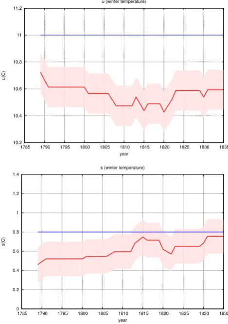
Fig. 5. Reconstruction of mean value (top), and standard devia-tion (bottom) of winter temperature for 31-yr running periods. The shadowed area represents the uncertainty range estimated using the model simulations for the whole millennium. Blue horizontal line: value corresponding to the reference period 1960–1990.
reconstruction yields the 31-yr running means and standard deviations. Four reconstructions were initially made using two reference periods and two pair of threshold valuesc. The reference periods chosen were 1885–1915 and 1960–1990. For each variable, a t-test for difference between means, an F-test for variances ratio, and a Kolmogorov-Smirnov test were performed to compare periods. The period 1885–1915 was significantly cooler in winter and wetter in spring and autumn (Table 4). For each reference period, two recon-structions were made, using as threshold valuescl andch,
the percentiles 10 and 90, and 25 and 75, respectively. Ta-ble 4 shows that these values may be very different, although there are no significant differences between periods (as, for instance, in the case of winter rainfall). The definitive recon-struction was obtained as the ensemble of the four individual reconstructions, and the associated uncertainty was estimated from the model simulations.
175 200 225 250 275 300 325
1700 1720 1740 1760 1780 1800 1820 1840
u (mm)
year u (winter rainfall)
25 50 75 100 125 150 175
1700 1720 1740 1760 1780 1800 1820 1840
s (mm)
year s (winter rainfall)
Fig. 6. As Fig. 5, for winter rainfall (green line: instrumental run-ning means).
The methodology allows low-frequency changes in the cli-mate variables to be reconstructed. Nevertheless, as will be seen below, it is possible to obtain high-frequency variabil-ity (interannual time-scale) when there is no gap between reconstructed and instrumental series.
Figure 5 shows the results corresponding to winter temper-ature for mean valueu(top) and standard deviation s (bot-tom), with the uncertainty bands determined by the RMSE within the model. Blue horizontal continuous lines indicate the value corresponding to the reference period 1960–1990. First, it may be seen that mean temperatures were slightly lower (up to 0.5◦C) than the modern value, with a minimum around 1815 and 1820. In the second place, the variability of winter temperatures is slightly lower than that of the ref-erence period, although it slightly increases to reach a peak around the same time interval, and at the end of the recon-structed period. The last result is yielded by the increasing number of observations at the end of the record.
Table 4. Main statistics of the reference period 1885–1915 (Twi = winter temperature (◦C); Rwi = winter rainfall (mm); Rsp = spring rainfall
(mm); Rau = autumn rainfall (mm);u= mean value;s= standard-deviation; ci = i-th percentile) and comparison with the period 1960–1990
(t-test, in parenthesis confidence interval for difference between means at the 95 % confidence level; F-test, in parenthesis confidence interval for variances ratio at the 95 % confidence level; KS = Kolmogorov-Smirnov statistic, in bold differences significant at the 95 % confidence level).
1885–1915
Twi Rwi Rsp Rau
u 10.6 228.3 190.1 210.9
s 0.7 102.7 75.9 70.4
c10 9.8 121.9 88.4 126.8
c25 9.9 154.4 132.2 174.9
c75 11.1 289.7 239.4 248.3
c90 11.5 332.4 282.2 299.0
Comparison between 1885–1915 and 1960–1990
Twi Rwi Rsp Rau
t-test 2.45 (0.09, 0.887) 0.16 (−58.5, 50.3) 3.60 (−95.3,−27.2) 2.43 (−88.6,−8.5)
F-test 1.10 (0.5, 2.3) 1.17 (0.56, 2.43) 1.78 (0.86, 3.70) 1.51 (0.72, 3.13)
KS 0.2581 0.0968 0.4194 0.3871
correlations. In all cases, the standard deviation recon-structed is lower than that of the reference period 1960–1990, except at the end of the series, probably as a consequence of the loss of variance in proxy data compared with instrumen-tal data. In the case of winter rainfall, the mean value of the complete period 1701–1850 (267±18 mm) was 19 % higher than during the reference period 1960–1990. The recon-structed values show minima around 1750, 1770, and 1790, an increase of rainfall in the first decades of the 19th century, and decreasing rainfalls at the end of the series. Compar-ison with contemporary instrumental running means at the end of the record shows that the magnitude of reconstruc-tions is similar to instrumental values. In this case, it must be borne in mind that instrumental values correspond mainly to Gibraltar, which is noticeably wetter than nearby sites in mainland Spain (Wheeler, 2007).
Figure 7 shows the reconstruction corresponding to spring rainfall. The gap corresponding to the first years of the 19th century is due to the absence of information on droughts (nl=0) from 1790 to 1824. The mean value for the
com-plete period (164±11 mm) was 27 % higher than during the reference period 1960–1990. The results show a dry period approximately between 1730 and 1790, with an increase of spring rainfall in the last decade of the 18th century and first decades of the 19th century. Comparison with contempo-rary instrumental running means shows that reconstruction slightly overestimates the instrumental values.
Figure 8 shows the reconstruction corresponding to au-tumn rainfall. The gap corresponds to the absence of infor-mation on droughts from 1782 to 1826 (nl=0). The mean
value for the complete period 1701–1850 (194±16 mm) was
19 % higher than during the reference period 1960–1990. The behavior of autumn rainfall is very similar to spring rain-fall, with a minimum in the period centered around the 1760s, and a progressive increase of precipitation from 1790s on-wards. Again, the reconstruction clearly overestimates in-strumental values. A possible explanation lies in the char-acter of rainfall during this season of the year, with an im-portant role of convective precipitation, that is, intense, short duration, local rainfall. In consequence, it may be the result of assigning an extreme character to the seasonal regional series when the event was strictly local, and limited to a few hours a day. A possible solution to this problem would be to refine the spatiotemporal resolution of the study, at least at the monthly time scale and for individual localities.
5 Discussion
100 125 150 175 200 225
1700 1720 1740 1760 1780 1800 1820 1840
u (mm)
year u (spring rainfall)
0 25 50 75 100
1700 1720 1740 1760 1780 1800 1820 1840
s (mm)
year s (spring rainfall)
Fig. 7. As Fig. 6 for spring rainfall.
snowfalls on 12 January 1820), the Mediterranean coast (snowfalls in Motril on 19 January 1816, frosts in Almu˜necar on 10–11 January 1830, frost in Malaga on 12 January 1850), and Seville (frosts on February 1822, 1823, and Decem-ber 1846, snowfalls on 7 February 1819 and February 1845). In addition, early instrumental data for Cadiz have allowed a first approach to the evolution of temperature in the region. As regards winter temperature, Wheeler (1995) found that winter temperatures of Cadiz from 1789 to 1816 were about 0.6◦C lower than modern data, a result similar to our recon-struction. Gallego et al. (2007) found that sunset tempera-tures taken in Cadiz for 1825–1852 show values as much as 2.7◦C lower relative to the 1971–2000 period from
Decem-ber to February. On the other hand, although it seems that the impact of the Tambora eruption on Iberia was more im-portant in summer (Trigo et al., 2009), a minimum in winter temperature has been detected around 1815–1820. Diodato et al. (2010) also found low temperatures in their reconstruc-tion of winter temperatures in central-southern Italy during the first decades of the 19th century. The analysis of early instrumental data in the region is a work in progress, but the first results seem to confirm, at least qualitatively, the validity of our reconstruction.
125 150 175 200 225 250
1700 1720 1740 1760 1780 1800 1820 1840
u (mm)
year u (autumn rainfall)
25 50 75 100 125 150
1700 1720 1740 1760 1780 1800 1820 1840
s (mm)
year s (autumn rainfall)
Fig. 8. As Fig. 6 for autumn rainfall.
values. Therefore, we must convert the mean values obtained into annual values. Running means may be expressed as
ut=
1 2r+1
k=r
X
k=−r
xt+k (4)
wherexis the annual value, and 2r+1=n(n=31,r=15 in our case). As a consequence, considering two consecutive running means, we obtain
xt−r=xt+r+1− −n(ut+1−ut) (5)
In this way, it is possible to obtain past annual values by means of an iterative process using instrumental values and running means. One inconvenience of this method is that the presence of gaps (in instrumental series or running means) propagates backward, preventing a complete reconstruction. This methodology was used for the winter and spring rainfall series (the number of gaps in autumn was very high), consid-ering that the instrumental series began in 1821, so that the first instrumental running mean is centered on 1836. There-fore, annual values were obtained from 1701 to 1820. Fig-ure 9 shows the comparison of the annual values obtained (z, expressed as standardized anomalies relative to the reference period 1960–1990) with the index series from rogations in Seville (I) for winter (a) and spring (b) during the same time period. Correlation coefficients are significant at the 95 % confidence level, but not very high (r=0.30), due to various factors: the I series are local, while the z series are regional; the existence of gaps in the instrumental series (1833, 1834, 1836, and 1837 in winter; 1824, 1825, 1833, 1836, and 1837 in spring) and the u series for spring (1805–1809, Fig. 7) multiply the number of gaps in past – in total, 16 (13.3 %) in winter and 34 (28.3 %) in spring – and the absence of infor-mation on rogations led us to assign an index valueI=0 in years in which the reconstruction shows positive and negative anomalies (for instance at the beginning of the 18th century in spring). However, at least from a qualitative point of view, the coincidence of positive and negative values is clear. Pos-itive values are detected, for example, in 1708, 1768, 1784, or 1808 (winter), and 1736, 1772, 1786 and 1804 (spring). Frequent droughts are found in 1737, 1753, 1789, and 1808 (winter), and 1722, 1737, 1750, 1780, and 1813 (spring). Indices obtained for southern Portugal for the 18th century (Taborda et al., 2004) also show positive values in 1708 and 1784 (winter), 1736 and 1786 (spring), and frequent droughts in winter 1737 and 1753.
Rogation ceremonies and rainfall information contained in documentary data are directly related to the behavior of crops, mainly wheat and barley. There is another important data source related to agricultural production: harvest taxes, or tithes. Every producer or owner had to pay 10 % of the total production either in kind or in money, after a public auction. This proxy was used to reconstruct precipitation in the Canary Islands for the period 1595–1836 (Garc´ıa et al., 2003). In Andalusia, a great number of tithes series have
39 1
2 Figure 9 3
(a)
(b)
39 1
2
Figure 9 3
(b)
Fig. 9. Comparison between reconstructed regional standardized anomalies (z) and rogation index of Seville (I) for winter (a), and spring (b), during the period 1701–1820.
been available after the compilation by Ponsot (1986), based on municipal and ecclesiastical archives of the Guadalquivir River Basin. For this work, we have used 22 series covering the period 1580–1837. The magnitude of tithes was different from one locality to another, depending of the extension of the farm area, and so the local series were standardized us-ing the mean value and standard deviation of the complete period. The next step was to construct a cereal production index Ic averaging the local indices. Figure 10 shows the
evolution ofIc from 1701 to 1820. As regards the
interpre-tation of such information, we must bear in mind that cereal production was not only related to climatic factors, but also to socioeconomic factors (agricultural techniques, political conflicts). In addition, the response of plants to climate is not linear, but depends on the different stages in the evo-lution of the plant, and is related not only to precipitation, but also to the appearance of frosts, heat waves, etc. How-ever, a qualitative comparison is possible, considering that
2 3
Figure 10 4
5
6
7
8
9
10
11
12
13
14
15
16
17
18
19
20
40
Fig. 10. Index of cereal production for the Guadalquivir River Basin, period 1701–1820. Red line: 11-yr moving average.
Table 5. Comparison between reconstructed standardized rainfall
anomalies of winter (zw)and spring (zsp) and cereal production
index (Ic), period 1701–1820.
Ic≤ −1 Ic≥ +1
Year zw zsp Year zw zsp
1734 −2.0 −8.8 1709 −2.0 Gap
1737 −0.8 −2.3 1719 −0.3 −0.8
1750 −0.3 −2.3 1725 +0.2 +3.1
1753 −2.0 −2.3 1735 +3.2 +1.2
1784 +0.1 −0.1 1741 −2.0 +4.3
1804 +0.3 +1.3 1746 −1.6 −0.4
1811 −1.1 −1.2 1755 −2.0 +2.7
1812 +0.2 +0.6 1766 +3.2 +1.2
1781 −2.0 −2.3
1782 −0.9 −1.2
1790 +0.6 Gap
1794 −1.4 Gap
1798 +2.8 +1.0
1802 −2.0 Gap
1808 −1.6 −0.4
Results are summarized in Table 5, showing the years with |Ic| ≥1 and the corresponding values of the reconstructed
rainfall anomalieszw andzspfor winter and spring,
respec-tively. Poor harvests (Ic≤ −1) are mainly related to drought
conditions, especially in spring, with droughts in the decades of 1730s and 1750s, although intense and/or continuous rain-falls may also affect the crops, as in 1784, 1804, and 1812. In particular, the 1783/1784 winter, with a severe flood in Seville, has been considered as typical for the Little Ice Age across much of Europe (Br´azdil et al., 2010a) and a flood in Granada was recorded on 9 May 1804 (Books of Acts of the City Chapter House). Good harvests seem to be related to rainy seasons or not very pronounced negative anomalies, as in 1746, 1782 or 1808.
0 0.2 0.4 0.6 0.8 1
6 8 10 12 14
T (C) Winter temperature
1790-1820 recons. 1960-1990 recons. 1790-1820 model 1960-1990 model
a)
0 0.001 0.002 0.003 0.004 0.005 0.006 0.007
0 100 200 300 400 500
R (mm) Winter rainfall
1790-1820 recons. 1960-1990 recons. 1790-1820 model 1960-1990 model
b)
Fig. 11. Density functions of the periods 1790–1820 (red) and 1960–1990 (blue) for winter temperature (a) and rainfall (b). Dashed lines correspond to model simulations.
An interesting exercise is the comparison between the Dal-ton Minimum period (approximately 1790–1820) and the reference period 1960–1990. Figure 11 shows the density function corresponding to both periods, accepting the nor-mality hypothesis, for winter temperature (a) and precip-itation (b). The continuous blue line represents the den-sity function of instrumental data for the period 1960–1990, and the red continuous line the reconstructed data for 1790– 1820. Dashed lines represent the density functions ob-tained from model simulations. The mean (standard devia-tion) temperature for the Dalton Minimum is 10.6 (0.5) and 8.3 (0.8)◦C in the reconstruction and the model, respectively,
model simulations clearly underestimate instrumental and reconstructed data (especially in the case of temperature). These biases are within the range of uncertainty characteris-tic of regional climate simulations, especially when the sim-ulations are not externally driven by observations, as is the case here. However, the simulation does not show such a large bias compared with other available observational data bases (G´omez-Navarro et al., 2011), which suggests that a complementary explanation for these biases is the presence of deficiencies also in the instrumental data employed in this study. Nevertheless, more important than biases, which are to a greater or lesser extent inherent in all models, is the am-plitude of climate variations in different climatic periods. In this respect it can be seen that both the reconstructed and sim-ulated climate show that the period 1790–1820 was colder and slightly wetter than the modern period 1960–1990. In the case of the model, this behavior is driven by the recon-structions of the external forcings, which show a decrease in the solar constant together with an increase of volcano ac-tivity during this period. Thus, the temperature and rainfall reconstructions for Andalusia presented in this study are in good agreement, qualitatively, with the Crowley’s (2000) re-constructions for global-scale forcings.
The Little Ice Age (LIA) is conventionally defined as a period extending from the 16th to the 19th centuries, though climatologists and historians working with local records no longer expect to agree on either the start or end dates of this period, which varies according to local conditions. The LIA can be considered as a modest cooling of the Northern Hemi-sphere of less than 1◦C relative to late 20th century levels (Crowley and Lowery, 2000). From dendroclimatic studies in Spain, Creus Novau (2000) found that the most important effect of the LIA in Spain was an increase of precipitation, with the tree-ring index showing increasing rainfall until the mid-19th century. The increase of rainfall in the first half of the 19th century (or, alternatively, the decrease in the quency of droughts) coincides with an increase in the fre-quency of floods in the Tagus river (central part of the IP, to the north of Andalusia) from 1780 to 1810 (Benito et al., 2003), and in Catalonia (NE IP) from 1830 to 1860 (Barrien-dos and Llasat, 2003). The LIA has been identified as the rainiest period at annual scale for the Mediterranean central area: in south Italy it was the stormiest period with high fre-quency of floods and erosive rainfall (Diodato et al., 2008) and for Greece, the period 1750–1820 was one of the wettest of the LIA (Xoplaki et al., 2001).
Precipitation anomalies over southern Spain are associated with pressure anomalies over the Atlantic Ocean northwest of the IP (Xoplaki et al., 2004; Pauling et al., 2006): nega-tive pressure anomaly facilitates advection of moist air from the Atlantic and low pressure triggers precipitation over the region; in the case of dry anomalies, this area is domi-nated by high pressure, which suppresses precipitation be-cause anomalous easterly winds over southern Europe pre-vent moist oceanic air from reaching southern Spain. Winter
precipitation over southern and central Spain is mainly deter-mined by the state of the North Atlantic Oscillation (NAO). In a study on the impacts of the NAO on Spanish rainfall dur-ing the 20th century, Mu˜noz-D´ıaz and Rodrigo (2004) found that changes in NAO phases led to changes in mean rainfall over this area, with important shifts in the probabilities of wet and dry seasons. This direct relationship between mean rainfall over the study area and NAO has been used for sea-level pressure (SLP) and NAO reconstructions (Luterbacher et al., 1999; 2002a, b; Rodrigo et al., 2001). In general terms, the results presented in this work are coherent with the monthly reconstruction of the SLP field from indepen-dent sources (Luterbacher et al., 2002b): greater meridion-ality in the general circulation, with more frequent cyclonic disturbances and northerly flows, being responsible for the wet and cold events detected, respectively.
6 Conclusions
The study presented here confirms the potential of using doc-umentary data in climatic reconstructions, at least with sea-sonal resolution. In addition, it is an example of the use of regional model simulations to test reconstruction methodolo-gies and results. Among the main results can be mentioned the reconstruction of winter temperature, a task that rarely appears in historical climatology studies focusing on the IP. Reconstructed winter mean temperature was slightly lower than the modern value, with a minimum around the period between 1815 and 1820. As regards rainfall, an increase of mean rainfall since the last decades of the 18th century has been detected. In this work, in addition to winter rain-fall, we have also presented reconstructions corresponding to spring and autumn, going beyond previous works that fo-cused on winter (Rodrigo, 2008) or total annual rainfalls (Ro-drigo et al., 1999). Comparison between the periods 1790– 1820 and 1960–1990 indicates that the former, i.e. the cen-tral interval of the Dalton Minimum period, was colder and wetter than the modern period. These results are in good agreement, at least from a qualitative point of view, with other reconstructions, based on other proxy data and regions (e.g. Barriendos and Llasat, 2003; Benito et al., 2003; Creus Novau, 2000; Diodato et al. 2010; Taborda et al., 2004; Xoplaki et al., 2001).
of extremes. Traditional reconstruction techniques based on ordinal severity indices assign the valueI=0 to these sit-uations. In this sense, the method followed here is more cautious, waiting for the analysis of new data sources be-fore attempting reconstruction process for periods with lack of news. Some features may be revised as, for instance, the choice of different reference periods, threshold values, or an adequate theoretical distribution function, instead of the nor-mal distribution. All these aspects, along with a deeper anal-ysis of possible relationships with climate forcings, will be studied in future works.
Appendix A
Documentary data sources
Data sources used in this work enlarge the list quoted in Ro-drigo et al. (1999) with these new references:
Medical topographies
Delgado, F.: Lecci´on hist´orico politico m´edica de las enfermedades que pueden seguirse de resultas de la pasada inundaci´on del Guadalquivir, in: Memorias Acad´emicas de la Real Sociedad de Medicina y dem´as ciencias de Sevilla, 3, 58–77, 1785.
Nieto de Pi˜na, C. J.: Historia de la epidemia de calenturas benignas que se experiment´o en Sevilla desde principios de Septiembre hasta fines de Noviembre de 1784, Biblioteca de Andaluc´ıa, sgn.: ANT-XVIII-406, 1785.
Nieto de Pi˜na, C. J.: Memoria de las enfermedades que se experi-mentaron en la ciudad de Sevilla en el a˜no de 1785, Biblioteca de Andaluc´ıa, sgn.: ANT-XVIII-407, 1786.
S´anchez, J.: Relaci´on de la epidemia de calentures p´utridas pade-cida en el nav´ıo de S.M. nombrado El Mi˜no en su viaje a Con-statinopla el a˜no de 1786, Biblioteca de la Universidad Com-plutense, Madrid, sgn.: BA-FOA-4747(3), 1789.
Gonz´alez, P. M.: Disertaci´on m´edica sobre la calenture maligna contagiosa que reyn´o en C´adiz el a˜no de 1800, Biblioteca Provincial de C´adiz, sgn.: XIX-5854(5), 1801.
Ar´ejula, J. M.: Breve descripci´on de la fiebre amarilla padecida en C´adiz y pueblos comarcanos en 1800, en Medisidonia en 1801, en M´alaga en 1803, y en esta misma plaza y varias otras del reyno en 1804, Biblioteca de Andaluc´ıa, sgn.: ANT-XIX-614, 1806. Mart´ınez y Montes, V.: Topograf´ıa m´edica de la ciudad de M´alaga. Biblioteca de Andaluc´ıa, sgn.: 1-N-965, 1852.
Newspapers
Semanario de Agricultura y Artes dirigido a los P´arrocos : Bib-lioteca de la Universidad de Granada, sgn.: B-81-31 to B-81-52, 1797–1808.
Diario Mercantil de C´adiz: Biblioteca Provincial de C´adiz, sgn.: FL-PP-Est.99, 1802–1812, 1816–1830.
El Publicista, Diario de Granada : Museo Casa de los Tiros, Granada, 1812–1813.
Diario del Gobierno de Sevilla : Biblioteca Nacional, Madrid, sgn.: R/60312(4)0269, 1812–1813.
Diario Constitucional de Granada: Museo Casa de los Tiros,
Granada, 1820.
Peri´odico de la Sociedad M´edico Quir´urgica de C´adiz: Biblioteca de la Universidad Complutense, Madrid, sgn.: BH MED Rev. 63, 1820–1822, 1824.
Diario de Sevilla : Biblioteca Nacional de Madrid, sgn.: sala PP, 1826–1831.
Diario de Sevilla de Comercio, Artes, y Literatura : Biblioteca de Andaluc´ıa, sgn.: P-ANT-8/1, 1829–1830.
El Indispensable de C´adiz: Biblioteca Nacional de Madrid, sgn.: ZR/784(10), 1838.
El Sevillano: Biblioteca Provincial de C´adiz, sgn.: PA-PP-6-D1, 1840.
Other sources
Anonymous: Nueva y tragica relaci´on. . . en la Bah´ıa de C´adiz en el espantoso Hurac´an, que se padeci´o los d´ıas 15 y 16 de Enero de este a˜no de 1752, Biblioteca Provincial de C´adiz, sgn.: BBH6C25-10, 1752.
Books of Acts of the City Chapter House: Archivo Municipal de Granada, vol L, CXLI, 1804.
Trigueros, C. M.: La Riada, descr´ıbese la terrible inundaci´on que molest´o a Sevilla en los ´ultimos d´ıas del a˜no 1783 i los primeros de 1784, Biblioteca de Andaluc´ıa, sgn.: ANT-XVIII-377, 1784. Tapia, J. B.: Breve descripci´on. . . en la tarde del d´ıa diez y siete de Mayo de 1789. . . Villa de Lora. . . por el beneficio de la lluvia, Biblioteca de Andaluc´ıa, sgn.: ANT-XVIII-377, 1789.
Ure˜na, M.: Observaciones meteorol´ogicas hechas en la isla de Le´on en 1803, in: Anales de Ciencias Naturales, vol 6, no.17, 224–244, no.18, 345–353, and no.19, 81–96, Biblioteca del Jard´ın Bot´anico, CSIC, Madrid, sgn.: P.0165, 1804.
Vel´azquez y S´anchez, J.: Anales de Sevilla. Rese˜na hist´orica. . . de 1800 ´a 1850, Biblioteca de la Real Academia de la Historia, Madrid, sgn.: 23/15604, 1872.
Matute y Gaviria, J.: Anales Eclesiasticos y Seculares de la muy noble y muy leal Ciudad de Sevilla, Biblioteca de la Real Academia de la Historia, Madrid, sgn.: 14/1012/1014, 1887.
Acknowledgements. This work was supported by the Spanish
Ministry of Environment (http://www.marm.es), project ‘Salv´a-Sinobas’ (reference number 200800050083542). Authors are in debt to M. Barriendos (University of Barcelona) for providing the rogations index series of Seville and to D. Wheeler (Univer-sity of Sunderland) for providing monthly rainfall data for Gibraltar.
Edited by: F. Dom´ınguez-Castro
References
Alcoforado, M. J., Nunes, M. F., Garc´ıa, J. C., and Taborda, J. P.: Temperature and precipitation reconstruction in southern Portugal during the late Maunder Minimum (AD 1675–1715), Holocene, 10, 333–340, 2000.
Barriendos, M.: Climate variations in the Iberian Peninsula during the late Maunder Minimum (A.D. 1675–1715): an analysis of data from rogation ceremonies, Holocene, 7, 105–111, 1997. Barriendos, M. and Llasat, M. C.: The case of the ‘Mald´a’ anomaly
in the western Mediterranean basin (AD 1760–1800): an exam-ple of a strong climatic variability, Climatic Change, 61, 191– 216, 2003.
Barriendos, M. and Rodrigo, F. S.: Study of historical flood events on Spanish rivers using documentary data, Hydrolog. Sci. J., 51, 765–783, 2006.
Benito, G., D´ıez-Herrero, A., and Fern´andez de Villalta, M.: Mag-nitude and frequency of flooding in the Tagus Basin (Central Spain) over the last millennium, Climatic Change, 58, 171–192, 2003.
Br´azdil, R., Pfister, C., Wanner, H., Storch, H., and Luterbacher, J.: Historical climatology in Europe-The State of the Art, Climatic Change, 70, 363–430, 2005.
Br´azdil, R., Demar´ee, G. R., Deutsch, M., Garnier, E., Kiss, A., Luterbacher, J., Macdonald, N., Rohr, C., Dobrovoln´y, P., Kol´ar, P., and Chrom´a, K.: European floods during the winter 1783/1784: scenarios of an extreme event during the “Little Ice Age”, Theor. Appl. Climatol., 100, 163–189, 2010a.
Br´azdil, R., Dobrovoln´y, P., Luterbacher, J., Moberg, A., Pfister, C., Wheeler, D., and Zorita, E.: European climate of the past 500 years: new challenges for historical climatology, Climatic Change, 101, 7–40, 2010b.
Br´azdil, R., Gonz´alez-Rouco, J. F., and Bronnimann, S.: Climate reconstructions based on instrumental, documentary, and natural proxy data, available at: http://meetingorganizer.copernicus.org/ EMS2011/session/8088, last access: 9 January 2012, 2011. Briffa, K. R., Osborn, T. J., Schweingruber, F. H., Jones, P. D.,
Shiyatov, S. G., and Vaganov, E. A: Tree-ring width and density data around the northern hemisphere: part I, local and regional climate signals, Holocene, 12, 737–757, 2002.
Brunet, M., Saladi´e, O., Jones, P., Sigr´o, J., Aguilar, E., Moberg, A., Lister, D., Walther, A., L´opez, D., and Almarza, C.: The devel-opment of a new dataset of Spanish daily adjusted temperature series (SDATS) (1850–2003), Int. J. Climatol., 26, 1777–1802, 2006.
Bull´on, T.: Winter temperatures in the second half of the sixteenth century in the central area of the Iberian Peninsula, Clim. Past, 4, 357–367, doi:10.5194/cp-4-357-2008, 2008.
Castro-D´ıez, Y., Esteban-Parra, M. J., Staudt, M., and G´amiz-Fortiz, S. R.: Temperature and Precipitation in Andalusia in the Iberian Peninsula and Northern Hemisphere context, in: Climate Change in Andalusia: trends and environmental consequences, edited by: Sousa, A., Garc´ıa-Barr´on, L., and Jurado, V., Junta de Andaluc´ıa, 57–77, 2007.
Creus Novau, J.: Dendrocronolog´ıa y dendroclimatolog´ıa, o c´omo los ´arboles nos cuentan el clima del pasado, in: La Recon-strucci´on del clima de ´epoca preinstrumental, edited by: Garc´ıa Codr´on, J. C., Universidad de Cantabria, Santander, 81–122, 2000.
Crowley, T.: Causes of climate change over the past 1000 years, Sci-ence, 289, 270–277, doi:10.1126/science.289.5477.270, 2000. Crowley, T. and Lowery, T.: How warm was the Medieval warm
period?, Ambio, 29, 51–54, 2000.
Diodato, N., Ceccarelli, M., and Bellochi, G.: Decadal and century-long changes in the reconstruction of erosive rainfall anomalies
in a Mediterranean fluvial basin, Earth Surf. Process. Landforms, 33, 2078–2093, 2008.
Diodato, N., Bellocchi, G., Bertolin, C., and Camuffo, D.: Mul-tiscale regression model to infer historical temperatures in a central Mediterranean sub-regional area, Clim. Past Discuss., 6, 2625–2649, doi:10.5194/cpd-6-2625-2010, 2010.
Dom´ınguez-Castro, F., Santisteban, J. I., Barriendos, M., and Me-diavilla, R.: Reconstruction of drought episodes for central Spain from rogation ceremonies recorded at the Toledo Cathedral from 1506 to 1900: A methodological approach, Global Planet. Change, 63, 230–242, 2008.
Dom´ınguez-Castro, F., Garc´ıa-Herrera, R., Ribera, P., and Barrien-dos, M.: A shift in the spatial pattern of Iberian droughts during the 17th century, Clim. Past, 6, 553–563, doi:10.5194/cp-6-553-2010, 2010.
Ebisuzaki, W.: A method to estimate the statistical significance of a correlation when the data are serially correlated, J. Climate, 10, 2147–2153, 1997.
Frei, C. and Sch¨ar, C.: Detection probability of trends in rare events: theory and application to heavy precipitation in the Alpine re-gion, J. Climate, 14, 1568–1584, 2000.
Gallego, D., Garc´ıa-Herrera, R., Calvo, N., and Ribera, P.: A new meteorological record for C´adiz (Spain) 1806–1852: im-plications for climatic reconstructions, J. Geophys. Res., 112, D12108, doi:10.1029/2007JD008517, 2007.
Garc´ıa, R., Mac´ıas, A., Gallego, D., Hern´andez, E., Gimeno, L., and Ribera, P.: Reconstruction of the precipitation in the Canary Islands for the period 1595–1836, B. Am. Meteorol. Soc., 81, 1037–1039, 2003.
Garc´ıa de Pedraza, L. and Garc´ıa Vega, C.: La sequ´ıa y el clima de Espa˜na, Calendario Meteorol´ogico 1989, Instituto Nacional de Meteorolog´ıa, Madrid, 1989.
G´omez-Navarro, J. J., Mont´avez, J. P., Jerez, S., Jim´enez-Guerrero, P., Lorente-Plazas, R., Gonz´alez-Rouco, J. F., and Zorita, E.: A regional climate simulation over the Iberian Peninsula for the last millennium, Clim. Past, 7, 451–472, doi:10.5194/cp-7-451-2011, 2011.
IPCC: The Physical Science Basis. Contribution of Working Group I to the Fourth Assessment Report of the Intergovernmental Panel on Climate Change, edited by: Solomon, S., Quin, D., Manning, M., Chen, Z., Marquis, M., Averyt, K. B., Tignor, M., and Miller, H. L., Cambridge University Press, Cambridge, United Kingdom and New York, NY, USA, 996 pp, 2007.
Lettenmaier, D.: Stochastic modeling of precipitation with applica-tions to climate model downscaling, In: Storch, H., and Navarra, A. (eds) Analysis of climate variability, Springer, Berl´ın, 197– 212, 1995.
Luterbacher, J., Schmutz, C., and Gyalistras, D.: Reconstruction of monthly NAO and EU indices back to A.D. 1675, Geophys. Res. Lett., 26, 2745–2748, 1999.
Luterbacher, J., Xoplaki, E., and Dietrich, D.: Extending North At-lantic Oscillation reconstructions back to 1500, Atmos. Sci. Lett., 2, 114–124, 2002a.
Luterbacher, J., Xoplaki, E., and Dietrich, D.: Reconstruction of sea-level pressure fields over the Eastern North Atlantic and Eu-rope back to 1500, Clim. Dynam., 18, 545–561, 2002b. Mart´ın-Vide, J.: Climate Change in Andalusia: trends and
Sousa, A., Garc´ıa-Barr´on, L., and Jurado, V., Junta de Andaluc´ıa, 1–5, 2007.
Mart´ın-Vide, J. and Barriendos. M.: The use of rogation ceremony records in climatic reconstruction: a case study from Catalonia (Spain), Climatic Change, 30, 201–221, 1995.
Mu˜noz-D´ıaz, D. and Rodrigo F.S.: Impacts of the North Atlantic Oscillation on the probability of dry and wet winters in Spain, Clim. Res., 27, 33–43, 2004.
Nash, J. E. and Sutcliffe, J. V.: River flow forecasting through con-ceptual models part I-A discussion of principles, J. Hydrol., 10, 282–290, 1970.
Pauling, A., Luterbacher, J., Casty, C., and Wanner, H.: Five hun-dred years of gridded high-resolution precipitation reconstruc-tions over Europe and the connection to large-scale circulation, Clim. Dynam., 26, 387–405, 2006.
Ponsot, P.: Atlas de Historia Econ´omica de la Baja Andaluc´ıa (Sig-los XVI-XIX), Editoriales Andaluzas Unidas, Granada, 1986. Rodrigo, F. S.: Changes in climate variability and seasonal rainfall
extremes: a case study from San Fernando (Spain), 1821–2000, Theor. Appl. Climatol., 72, 193–207, 2002.
Rodrigo, F. S.: A new method to reconstruct low-frequency climatic variability from documentary sources: application to winter rain-fall series in Andalusia (southern Spain) from 1501 to 2000, Cli-matic Change, 87, 471–487, 2008.
Rodrigo, F. S. and Barriendos, M.: Reconstruction of seasonal and annual rainfall variability in the Iberian Peninsula (16th–20th centuries) from documentary data, Global Planet. Change, 63, 243–257, 2008.
Rodrigo, F. S., Esteban-Parra, M. J., and Castro-D´ıez, Y.: On the use of the Jesuit Order pr´ıvate correspondence records in climate reconstructions: a case study from Castile (Spain) for 1634–1648 A.D., Climatic Change, 40, 625–645, 1998.
Rodrigo, F. S., Esteban-Parra, M. J., Pozo-V´azquez, D., and Castro-D´ıez, Y.: A 500-year precipitation record in southern Spain, Int. J. Climatol., 19, 1233–1253, 1999.
Rodrigo, F. S., Esteban-Parra, M. J., Pozo-V´azuqez, D., and Castro-D´ıez, Y.: Rainfall variability in southern Spain on decadal to cen-tennial time scales, Int. J. Climatol., 20, 721–732, 2000. Rodrigo, F. S., Pozo-V´azquez, D., Esteban-Parra, M. J., and
Castro-D´ıez, Y.: A reconstruction of the Winter North Atlantic Oscilla-tion index back to A.D. 1501 using documentary data in southern Spain, J. Geophys. Res., 106, 14805–14818, 2001.
Rutherford, S., Mann, M. E., and Osborn, T. J.: Proxy-based North-ern Hemisphere surface temperature reconstructions: sensitivity to method, predictor network, target season, and target domain, J. Climate, 18, 2308–2329, 2005.
Solow, A. R.: On testing for change in extreme events, Nature, 316, 106–107, 1999.
Taborda, J. P., Alcaforado, M. J., and Garc´ıa, J. C.: The climate
of southern of Portugal during the 18t hcentury: a reconstruction
based on descriptive and instrumental sources, Geoecologia, Rel. 2, Centro de Estudos Geograficos, Lisboa, 2004.
Trigo, R. M., Vaquero, J. M., Alcoforado, M. J., Barriendos, M., Taborda, J., Garc´ıa-Herrera, R., and Luterbacher, J.: Iberia in 1816, the year without summer, Int. J. Climatol., 29, 99–115, 2009.
Vicente-Serrano, S. M. and Cuadrat, J. M.: North Atlantic oscil-lation control of droughts in north-east Spain: evaluation since 1600 A.D., Climatic Change, 85, 357–379, 2007.
Wagner, S. and Zorita, E.: The influence of volcanic, solar, and CO2
forcing on the temperature in the Dalton Minimum (1790–1830): a model study, Clim. Dynam., 25, 205–218, 2005.
Wheeler, D.: Early instrumental weather data from Cadiz: a study of late eighteenth and early nineteenth century records, Int. J. Climatol., 15, 801–810, 1995.
Wheeler, D.: The Gibraltar climatic record: Part 2- precipitation, Weather, 62, 99–104, 2007.
Wilks, D. S.: Statistical methods in the atmospheric sciences, Aca-demic Press, San Diego, 1995.
Xoplaki, E., Mahera, P., and Luterbacher, J.: Variability of climate in meridional Balkans during the periods 1675–1715 and 1780– 1830 and its impact on human life, Climatic Change, 48, 581– 591, 2001.
Xoplaki, E., Gonz´alez-Rouco, J. F., and Luterbacher, J.: Wet season Mediterranean precipitation variability: influence of large scale dynamics and trends, Clim. Dynam., 23, 63–78, 2004.
Zhang, X., Aguilar, E., Sensoy, S., Melkonyan, H., Tagiyeva, U., Ahmed, N., Kutaladze, N., Rahimzadeh, F., Taghipour, A., Han-tosh, T. H., Albert, P., Semawi, M., Ali, M. K., Al-Shabibi, M. H. S., Al-Oulan, Z., Zatari, T., Khelet, I. A. D., Hamoud, S., Sa-gir, R., Demircan, M., Eken, M., Adiguzel, M., Alexander, L., Peterson, T. C., and Wallis, T.: Trends in Middle east climate ex-treme indices from 1950 to 2003. J. Geophys. Res., 110, D22104, doi:10.1029/2005JD006181, 2005.