www.nonlin-processes-geophys.net/17/237/2010/ © Author(s) 2010. This work is distributed under the Creative Commons Attribution 3.0 License.
Nonlinear Processes
in Geophysics
Kernel estimation and display of a five-dimensional conditional
intensity function
G. Adelfio
Dipartimento di Scienze Statistiche e Matematiche “Silvio Vianelli”, University of Palermo, Palermo, Italy Received: 3 December 2009 – Revised: 29 January 2010 – Accepted: 8 February 2010 – Published: 22 April 2010
Abstract. The aim of this paper is to find a convenient and
effective method of displaying some second order properties in a neighbourhood of a selected point of the process. The used techniques are based on very general high-dimensional nonparametric smoothing developed to define a more gen-eral version of the conditional intensity function introduced in earlier earthquake studies by Vere-Jones (1978).
1 Introduction
This paper is concerned with the second order properties of a multidimensional point process in contexts where some fea-tures of a given point (e.g. location, depth, magnitude) play a dominant role in determining the local behavior of the pro-cess in a neighbourhood of the selected point. The aim of the paper is to describe a convenient and effective method of displaying second order properties of counts in a neighbour-hood of a selected point of an observed point process and to examine how those properties are affected by the features of the fixed point. In particular we would like to display second order properties of counts in a neighbourhood of the initial event in an aftershock sequence or swarm in a seismic active area. For instance, the way these properties change with the magnitude of the initial event tells us something about the physical processes governing the numbers and distributions of the aftershocks respond to the size of the initial event. Similar issues arise in the discussion of medical epidemic data, where the size and severity of the epidemic overall may be related to characteristics of the initial recorded infection.
To look at second order properties, the counts need to be averaged over both the choice of a selected point and over the events in its neighbourhood. Ripley’s K-function (Ripley,
Correspondence to: G. Adelfio
1976) is commonly used for such a purpose in discussing the cumulative behavior of interpoint distances about an initial point. It is defined as the expected number of events falling within a given distanceδ of the initial event, divided by the overall density (rate in 2-dimensions) of the process, sayλ. Since it is defined as an average over many initial points, the K-function cannot be used to distinguish processes with the same (average) second order properties. As an alternative, Getis and Franklin (1987) suggested examining the behavior of the occurrence patterns in the neighbourhood of selected initial points developing a second order neighbor analysis of mapped point patterns. However, this method is not use-ful for determining whether a given pattern is random, clus-tered or regular (Doguwa, 1989). Adelfio and Schoenberg (2009) suggested using a weighted version of some second order statistics to provide diagnostic tests. In Adelfio and Chiodi (2009) weighted second order statistics are used to assess the fitting of seismic models to real catalogs. Gril-lenzoni (2006) focussed on the conditional intensity function of a space-time process, where conditioning is made on the basis of past events only.
In this paper a nonparametric estimation of the second or-der conditional intensity function (CIF) introduced by Vere-Jones (1978) is provided, by making use of kernel intensity estimators. The nonparametric second order CIF is here in-troduced to analyze the influence in a neighbourhood of a multidimensional point to some properties of the observed point pattern, by using a procedure that does not require any constraining assumption to characterize the generating pro-cess.
In Sect. 2 a brief introduction of spatial-temporal point processes and their second order characteristics is pro-vided. The proposed nonparametric approach is introduced in Sect. 3, showing some application in Sect. 4. Section 5 provides some concluding remarks and directions for future study.
2 Point processes and conditional intensity function
A spatial-temporal point process is a random point pattern defined by time and location of every single event. Point processes are here introduced by a mathematical approach that uses the definition of a counting measure on a setX⊆
Rd,d≥1, with positive values inZ: for each Borel set B
thisZ+-valued random measure gives the number of events
falling inB.
This section reviews some basic definitions related to point processes, reported to introduce the notation used throughout the paper. For further elaboration and references, please see Daley and Vere-Jones (2003).
Definition 1 Point process
Let(,A,P )be a probability space and8a collection of
locally finite counting measures onX⊂Rd. DefineX as the
Borelσ-algebra ofXand letN be the smallestσ-algebra on
8, generated by sets of the form{φ∈8:φ (B)=n}for all
B∈X. A point processNonXis a measurable mapping of
(,X)into(8,N). A point process defined over(,A,P )
induces a probability measure5N(Y )=P (N∈Y ),∀Y∈N
(Cressie, 1991).
Given a point processN defined on the space(X,X)and a Borel setB, the number of pointsN (B)inBis a random variable with first moment defined by:
µN(B)=E[N (B)] = Z
8
φ (B)5N(dφ)
that is a measure on(X,X). The measureµN is called the
mean measure or first moment measure ofN(Cressie, 1991). The second moment measure ofN is given by:
µ(N2)(B1·B2)=E[N (B1)N (B2)] =
Z
8
φ (B1)φ (B2)5N(dφ),
withB1,B2∈X. If it is finite inX(2)the process is second order.
Letds anddu be small regions located ats andu∈X, and let`(x)be the Lebesgue measure ofx. The first order
intensity is defined by:
η(s)= lim
`(ds)→0 µN(ds)
`(ds) ;
the second order intensity is defined by:
η2(s,u)= lim `(ds)→0 `(du)→0
µ(N2)(ds·du) `(ds)`(du) .
The second-order counting properties of such a process can be summarized by a covariance density:
c(s,u)ds du=Cov{N (ds),N (du)}, (s6=u). (1) The covariance measure also has a singular component concentrated along the lines=u, as illustrated by the for-mula:
Var{N (ds)} =E[N (s)]=µN(s).
LetN be a point process on a spatial-temporal domainX=
R+×Rd, d≥2; the functionλ∗(t,z)=λ(t,z|Ht), defined
by:
λ∗(t,z)= lim `(dt )→0 `(dz)→0
E[N ([t,t+dt )·[z,z+dz)|Ht)]
`(dt )`(dz) ,
(2) is the intensity function of the process conditioned to Ht,
that is the space-time occurrence history of the process up to timet, or in other words, theσ-algebra of events occurring at times up to but not includingt;dt,dzare time and space in-crements respectively, andE[N ([t,t+dt )× [z,z+dz)|Ht)]
is the history-dependent expected value of occurrence in the volume {[t,t+dt )× [z,z+dz)}. The conditional in-tensity function is a function of the point history and it is itself a stochastic process depending on the past up to timet. Assuming such a limit exists for each point (t,z) in the space-time domain and the point process is simple, the conditional intensity process uniquely characterizes the finite-dimensional distributions ofN (Daley and Vere-Jones, 2003). According to the used notation, the star inλ∗(·)is used to indicate that the intensity is a function of the past historyHt.
In a time-stationary but spatially inhomogeneous process, the expression in (2) is:
λ∗(t,z)=λf∗(z)
withλthe overall rate occurrence for a given region andf (·) a time-invariant space density. A more general form for (2) is provided assuming a separable form, in which the spatial term is assumed to be univariate in time and temporal density is not constant, where the both terms are allowed to depend on the past history, such that:
λ∗(t,z)=λ∗(t )f∗(z) (3) It simplifies to the product of constants for homogeneous Poisson processes.
In this paper a nonparametric estimation of a second or-der measure like (3) is provided to describe dependency structures of a multidimensional observed seismic process by using a flexible procedure based on kernel intensity estima-tors.
3 Nonparametric estimation
For an adequate description of the seismic activity of a fixed area and to suggest useful ideas on the mechanism of a such complex process, the definition of a valid and effective model is required. When a complete definition of a parametric model is not reliable, nonparametric approach could be use-ful. Indeed, in seismic modelling contexts, parametric mod-els are not always useful since the definition of a reliable mathematical model from the geophysical theory may not be available.
In general, some disadvantages of the parametric mod-elling can be avoided by using flexible procedures (nonpara-metric techniques), based on kernel intensity methods (Sil-verman, 1986). Given n observed events s1,s2...,sn in a
d-dimensional given region, the kernel estimator of an un-known densityf inRdis defined as:
ˆ
f (s1,...,sd;h)= 1 nhs1...hsd
n X
i=1 K
s1−s i1 hs1
,...,sd−sid hsd
(4) where K(s1,...,sd) denotes a multivariate kernel density (usually the standard Normal density function) operating on darguments centered at(si1,...,sid)andh=(hs1,...,hsd)
0is
the vector of the smoothing parameters of the kernel func-tions. If si = {ti,xi,yi,zi,Mi}, the space-time-magnitude
kernel intensity estimator of (2) is defined by the superpo-sition of the separable kernel densities:
ˆ
λ(t,x,y,z,M;h)∝
n X
i=1 Kt
t−t i
ht
·Ks
x−x i
hx
,y−yi hy
,z−zi hz
KM
M−M
i
hM
(5)
whereKt,Ks andKM are temporal, spatial and magnitude kernel density functions, as in (4), respectively.
Introducing the estimator defined in (5), the estimation of a complex intensity function dependent on the past history of the process as in (2) now reduces to the estimation of the intensity function of an inhomogeneous Poisson process, in-dependent of the past history and identified by a space-time Gaussian kernel intensity (Adelfio and Ogata, 2010); this re-sult provides useful directions for a simpler estimation ap-proach in describing very complex phenomena such as the seismic one. Separability of time and space kernel densi-ties is here assumed for computational convenience, because of the high dimensional issue, although tests to assess this assumption could be used (Schoenberg, 2004). It might be useful to note that this assumption is not directly extended to the intensity function of the process since it is obtained by the superposition of these densities.
In this context the problem of choosing the amount of smoothing is of crucial importance, since smoothing parame-ter regularizes the trade-off between variance and bias of the estimator, that is between random and systematic error. In Adelfio et al. (2006) the seismicity of the Southern Tyrrhe-nian Sea is described by Gaussian kernels and the optimum value ofhis chosen such as to minimize the mean integrated square error (MISE) of the estimatorf (ˆ ·). In particular the authors used the valuehoptthat Silverman (1986) obtained minimizing the MISE off (ˆ ·)assuming multivariate normal-ity.
In Adelfio (2010) a variable bandwidth procedure is in-troduced, choosinghj=(hjx,h
j y,h
j
t), i.e. the bandwidth for
thej-th event,j=1,...,n, as the radius of the smallest cir-cle centered at the location of thej-th event(xj,yj,tj)that
includes at least a fixed number of further events.
In Adelfio and Ogata (2010) a naive likelihood cross-validation function is optimized to obtain the bandwidth of the smoothing kernel used to estimate the intensity for earth-quake occurrence of northern Japan.
Although the use of variable bandwidth may be preferable to reflect local occurrence rates instead of using fixed band-width, in this paper constant smoothing is considered as a convenient approach to deal with the high dimensionality of the analyzed problem.
3.1 Conditional intensity estimation
A discrete estimate of the second order conditional inten-sity for a point process is given by Vere-Jones (1978). Now we are looking for a smoothed version of the conditional in-tensity, that is the local intensity of the process atp, given the occurrence of a point of the process ats. Thus:
h(p|s)dp=E[N (dp)|N (ds)=1] (6) wheresandpare points inRd, withd=5, since we are
con-sidering space (3-D), time and magnitude dimensions. This function can be related to the covariance density (1) by the equation
h(p|s)=µN(p)+c(p,s)/µN(s).
Moreover the formula above can be considered as another way of looking at the Ripley’s K-function, useful when the emphasis is on the physical interpretation of the dependence. In this paper nonparametric kernel estimators are used for estimatingh(p|s)in high-dimensional domain; in this con-text the conditioning puts a different complexion on the prob-lem, as the smoothing parameters have to be adjusted to the conditioning event.
Here we use a version of the conditional intensity func-tion introduced in earlier earthquake studies by Vere-Jones (1978), where the second order properties are classified ac-cording to the magnitude of the initial event. In the early paper the analysis was based on a crude discretization of the process, but in the present paper we make use of kernel den-sity estimates applied jointly to both the conditioning and the conditioned events. More precisely, to evaluate a smoothed version of the conditional intensity (CIF) in (6), we use the ratio estimate
ˆ h(p|s)=
ˆ λ(p,s)
ˆ
λ(s) (7)
that is, the ratio between the joint intensity of the condition-ing and the conditioned event (i.e.pands), and the marginal intensity of the conditioning event (events). This function is therefore estimated as the ratio of the kernel intensity esti-mators, defined in Eq. (5), forλ(p,s)andλ(s), respectively. The kernel estimators consider Gaussian density with zero mean and variance selected in a such way that its standard deviationh(the kernel bandwidth) minimizes the mean inte-grated square error (MISE) of the estimateλ(ˆ ·).
This approach simplifies the complex estimation issue of the second-order measure in (6), although it implies the use of high dimensional kernel functions. Indeed, the quan-tity in (7) has been computed considering the ratio of five-dimensional kernel estimators, providing, on one hand, a very computer intensive procedure, but on the other hand, some advantages related to the possibility of describing the main features of the process in multiple domains without constraining data to binding assumptions.
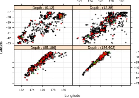
Longitude Latitude −43 −42 −41 −40 −39 −38 −37 * * * * * ** * * * * * * * * * * * * * * * * * * * * * * * * * * * * * * * * * * * * * * * * * * * * * * * * * * ** * ** * * * ** ** ** * * * * * * * * * * * * * ** ** * ** * * * * * * * ** * ** ** * * * * * * * * * * * * *** * * * * * * * * * * * * * ** * * * * * * * * * ** * * ** **** ************************************************* ** * ** * ** * * *** * * * * * * * *** * * * * * * * * ** ** * * * * **** * ** * * * * * * * * * * * * * ** * * * * * * * * * * * * * * ***** * * * * *** ** * * * * * * * * * * ** * ** ** * * * * * * * * * * ** * ** ** * * ** * * * * * * * * * * * ** ** * * * * * * * ** * * * ** **** ** * *** * * * * * * * * * * * * * * ** * ******** * * * * * * * * *** ***** * * * ** ** * ******* * * * * * * * * * * * * *** **** **** ** *** *** ******** * ******************************************************************************************************************************************************************************************************************************** * * ** ********** ****** * **** * * * **** ****** * * * * * * * * * * * * * * * * * *** * * * * * * * ** * * * * * * * * * * * * * * * * * * ** * * * * * ** * ***** * * * * ** ** * ** * * * * * * * * * * * * * * * * * * * * * * ** * * * * * * * * * * * * * * **** ************************* ** ** * * * ** : Depth (0,12]
172 174 176 178 180
* * * * * * * * * ** * * * * * * * * * * * * * * * * * * * * * * * * * * * * * * * * * * * * * * * * * * ** * * * * * * * * * ** * * * * * * * * ** * *** * * * * * * * * * * * * * * * * * * * * * * * * * * * **** * * * * *** ** * * * * * * * * * * * * * * * * * * * * * * * * * * * * * * * * * * * * ** * * * * * * * ** * * * * * * * * ** ** * ** * * * * * * * * * * * * * ** * ** * * * * ** * * * * * ****** * ** * * * * * * * * * * * * * * * * * * * * * * *** **** *** ** ** * * * * * * * * * * * * * * * * * * * * * * * * * * ** * * * * * * * * * * * * * ** * * * * * * *** * * ******* * * * * * * * ** * * * * * * * * * * * * * * * * * * * * * * * * * *** * * * * * * * ** * * * * * * * * * * ** * * ** * * * * * * * * * * ** * ** * * * * * * * * ** * * * * * * * * * * * * * * * * * * * * * * * * * * * * * * * * * * ** * * * * * * * * * * * * * * * * * * * * * * * * * * * * * * * ** * * * * *** * * * * * * * * * * * ** * * * ** * ** * ****** *** * * * * **** *** ** * ** * * * * * * * * * * * * * * * * * * * ** * ** * * * * * * * * * * * * * * ** * * * * * * * *** * * * * ** * * * * * * * * * * * * ** * * * * * * * * * ** * * * * ** * * * * * * * * * * * * * * * * * * ** * * * * *** * * * * * * * ** * * * ** * * * * * * * * * * * ** * * * * : Depth (12,85]
172 174 176 178 180
* * ** ** * * * * * * * * ** * * *** ** * * * * * * * * * * **** * * * * * * * * * * * * * * * * * ** * * * * * * * * * * ** * * * * * ** * ** * * * * ****** * * * * * ** ** * *** ** * * * * ** * * * * ** * * ** * * * * * * * * * * * * * *** * ** * ** * * * * ** * * ** ** * ** ** * * * * * * * * * * ** * * * * * * * * * * * * * ** ** ** * * * * * * * * * * * * ** * * * * * * * * * * * * * * * * ** * * * * * * * * * * * * ** * * * *** * * ** * * * * * * * * * * * * * * * * * * *** ** * ** * * * * ** * * * * * * * * * * * * * * * * * * * * * * * ** * * * * ** * * * * * ** * * * * ** * * * * * * * ** * * * * * * *** * * * * * * * * * * * * * * * * * * * * * ** * * * * * * * ** * *** * ** * * * * * ** * ** * * * * * * * * * * * * * * * ** * * * * * ***** * * * * * * * ***** * ** * *** * * ** * * * ** * * * * * * * * * * * *** ** * * * * * * ** * * *** * ** * * * * * * * * * ** * * * * ** * * * * * * * * * * * * * * * * *** * * * ** * ** **** * * * * * * * * * * * * * * ** * * * * * * * * * * * * ** * * * ** * * * * * * *** * * *** * * * * * ** * * * * * * * * * * *** * *** * * * * * * ** * * * * * * * * ** * * * * * * * * * * * ** * * **** * * * * * * * * * * * * * * * * * * * * * * * * ** * * * * * ** * * * * * * * *** ** * * ** * * * * * * * * * * * ** ** * * * * * * * * * * * * * * * * * * ** ** * * * * * *** * * * * * ** * * * * * * * ** * * * * * * * * * * * ***** * * * * * * * * * * * * * : Depth (85,186] −43 −42 −41 −40 −39 −38 −37 * * * * * * ** *** * * ** * * ** ** *** * * * * * *** * * * * * * * * * * * * * * * * * * ***** * * * * ** * * * * * * * ** * * * * * * *** * ** * * ** * * * * * * ** *** * ** * * *** * * * * * * * * * * * * * * ** * * * ** * * * * * * * * * * * * ** * * ** * *** * * * * * * ** **** * * ** *** * * ** * * * **** ** * * *** * * * ** * * * ** * ** * * *** * * * * * * * * * *** * * * * * * * ** * ** * * * * * * *** * *** * * * * * * * * * * ** * *** * * * * * * * ** ** * ******** * * * * * * * * ** * * * * ** * * * * * * * * ** * * * *** * * * * * * * * * * * * ** * * * * * ** * * * ** * * * * * * ** * * * * * * * * **** * ** ** ** * * ** * ** * * * * * * * * * * * * *** * * * ** * * * ** ** ** *** * * * * ** * ** * * * ** * * * ** ******* * ** ** * * * * ** * * * * * ** * * * * * * ** ** ** * * * * ** ** * * * * * * * * * * * * ** * * * * * ** * * * * * * * ** * *** * ** * ****** * * * * * * * **** * * * ** * * * * * * * * ** * ** *** * * ** * * **** ** * * * * * ** *** * * * **** * * ** * * * * * * ** * * ** ** ** * * * *** ** ** * * * * * * * * * ** * * *** * * * ** * * * * * *** *** * * *** * * * * * * *** * * ** * * * * * * * * * * * ** * * * * **** * ** * * * * *** * ** * * * * * ** * * ** * ** * * ** * * * * * * * * * ** * * *** * * * *** * * * * * * ** * * * * * * ********* ** * ** * * * * * *** ****** ** * * *** * * : Depth (186,602]
Fig. 1. 3-D space plot, with depth discretized into four groups with
equispaced quantiles as breakpoints, so that all groups have roughly the same number of points. Different colors are used for different ranges of magnitude: black for 4.5≤M <5.4, red for 5.4≤M <
6.3 and green for 6.3≤M <7.2.
4 Application to New Zealand data and discussion
Space-time modelling seems one sensible direction, espe-cially if depth is also involved. Some pictures could suggest something about the evolution of spatial clusters at various depth (when they merge or separate). Deep earthquakes gen-erally lack fully evolved sequences which decay according to the Omori’s law Utsu (1961). Therefore clustering described from ETAS model (Ogata, 1988) could be valid just for shal-lower events, that may have a classical aftershocks behavior. On the other hand, aftershocks for deep events have a differ-ent behavior and for this case a differdiffer-ent modelling could be useful, mostly to check their features that are still unknown in some sense.
Here a direct approach to analyze second order properties of deep earthquakes is considered, based on the use of the two point correlation function, that is of the conditional in-tensity function defined in (7).
We selected a subset of the GeoNet catalog of New Zealand earthquakes. Completeness issues of this catalog are discussed in Harte and Vere-Jones (1999). The data con-sist of n=3097 earthquakes of local magnitudeML=4.5 and larger that are chosen from the wide region−43◦∼ −37◦N and 171◦∼181◦E and for the time span 1951∼2007. That area is characterized by several deep events, with depth down to 530 km.
The bandwidth constants selected for the five-dimensional intensity kernel estimator of the process arehx=0.34,hy=
* * * * * * * ** * * * * ** * * * * * * * * * * * * * * ** * * * * * * * * * ** * * * * * * * * ** * ** * * * * * * * * ** * * * * * * * * * ** * * * ** * * * * * * * * * * * ** * * * ****** * * **** *** ** ******** * ***** * ** * **** *** * ** * * *** * * ******* *** *** * **** * *** * * * ***** * * * * * * ****** * * * * *** * *** ** * ** * ************ * * * * ** * ** * ***** * * **** * * * * **** ** ********** * *** * * * *** * ** ******* * **** **** * *** *** ** ** ************ * **** * *** ****** * ** * ** * * * * ** **** * ******** * *** * **** **** * * *** *** * * * * **** *** *** * * **** * * * ** * **** * * *** * ***** * * * *** * * * *** * * * * * * * * ** * * * ** * * ** * * ** **** * * * *** ** * * ** * * * * * * * * ** * * * * * ** * * * * ** * * * * * ** * * ** ** * * * * ** * * * * * * * * * * * * * * ** * * * * * * * * * * * * * * * ** * * ** * * * * * * * * * ** * * * * * * * * * * * * ** * * * ** * *** * * * * * * * * * * * ** * ** * * * * ** * * * ** ** ** * * * * * * * * * * * * * * * * * ** * * * * ** * ** * * * ** * * * * * * ** * ** * * * * * * * * * * * * *** * * * * * * * * * * * * * * * * * ** * * * * * * ** * ** * * * * ** * * * *** * * * * * * ** ****** * * * * ***** ******* **** * * ******************** * ******* * * ** ** * * * * * * * * * * * * * *** * * * * ** * * * * ** ** * * * * * * * * * * ** * * * *** ** * *** * * * * ** * * * * * * * * * * * ** * ** ** * * * ** * * * * *** * * ** * 172 175 178 181 −42 −40 −38 −37 1951 1965 1979 1993 2007 Longitude Latitude Time : Depth (0,12] * * * ** * * * * * * * * ** * * * * * * ** ** ** * * * ** * ** * * * * * * * * * * * * * * * * * ***** * * * * * * ** * * * * * * * * * * * * * * * * * * * ** * * * ** * * ** * * * * *** * * * * * * * * * * * ** * * ** * * * * * * * * * * ** * * * * * * * * * * * * * * * * * * * * * * * * * * * * * * * * * * * * * * * * * * * * * * * * * * * * * ** * * * * * * * * * * * * * * * * * ** * ** * ** * * * * * * * ** * * * * * * ** * * * * * * * * * * * ** * * * * ** * * * * * * * * * ** * * * * * * * ** * * *** * ** * * * * * * * * * * * * * * * * * * * * * * * * * * * * * * * * * * * * *** ** * * * * * ** * * * * * * * * * * * * * * * * * * * ** * * * * ** * * * * * * * * * * * * * * * * * * * ** * * * * * * * * * * * * * * * * * * * * *** * * * * * * * * * * * * * * * * * * * * * * * * * * * * * ** * * * ** * ** * * * * * ****** * * * *** * * * * * * * * * * * * * * * * * * ** ** * * ** ** * * * * * * ** * * * * * * * ** * * * ** * * * * * * * * ** * * * * ** * * ** * * ** * * * * * * * * * *** * * * * * * * * ** * ** *** * * * ** * * * * * * * * * * * * * * * * * * * * ** * ** * * * * * **** * * ** * ** * * ** * ** ** ** * * *** ** * * * * * * * * * * * * * * * * * * * * * * ** * ** * * * * * * * * * * * * ** * * * *** * *** ***** 172 175 178 181 −42 −40 −38 −37 1951 1965 1979 1993 2007 Longitude Latitude Time : Depth (12,85] * * * ** * ** * * ** ** * * * * * *** * * * * * * * * * * * * * * * ** * * * *** * * * * * * * * * * * * * * * * * * * * * * * * *** ** *** * * * * ** * * * * * * * * ** ** * * *** * * * * * * * * * ** * * * * * * * * * * * * ** * * * *** * * * *** * * ** * * * * * * * * * * * * * * * * * * *** * ** * *** * ** * ** ** * * **** * * * * ** * * * * * * * ** ** ** *** * * * * ** * * ** * * * * ** * * * * * * * * * * * * * * * ** * * * ** ** ** ** * * * *** * * * * * ** * * * * ** * * * * * * * * * * * * * *** * * ** ** ** * * * * * * * * ** * * * ** * * * * * * * * * *** * * * ** * * * * * * ** * * *** * * *** * * * * *** * * * **** * * * * * * * * * * * * * * ** * * * * * * * * * * * ** * * * ** * * * * ** * * * * ** ** * * * * * * * * * * * * * * * * * * * * * * * ** * ** * * * ** * * * * * * * * * * * * ** ** ** * * * * * * ** * * * ****** * * * ** * * * ** * * * * * * ** * * * * * * * * ** * ** * * * ** * * * * * * * * * * * **** * * * * **** * * *** * * * * * * ** * * * * * * * * * * * * * ** * * * * * * * * ** * * * * * **** * * * * * * ** * * * ** * ** * * * ** * * ** * ** * * * * ** * * * * * ** * * * ** * * * * * * * * * ** * * * * * * * ** * * * * * * * * * * * * * * * * * * * * * * * * * * * * * * * * * * ** ** ** * * * * * ** * * ** * * * * * * * *** * * * * * * * * * * * * * * * ** * *** * * * * * * ** *** * * * * * * **** * * * ** * * * * ** * * * * * * * **** *** 172 175 178 181 −42 −40 −38 −37 1951 1965 1979 1993 2007 Longitude Latitude Time : Depth (85,186] * * ** ****** * * *** * * ** ***** ** ** * ** ***** * * * * * * * * ** * * *** ** * * * * * **** * * * * * * ** * * * ** * ** * * * * * **** * ** * * * * * * * ** * * * * * * * * * * ***** * * *** * * ** * * * * * * * * * * * * ****** * * * ** * * * ** * * * * ** * ** * * * * * * * * * ** * * * * ** * * ** * * * * *** * * ** * * * * *** * * * * * * * * * * * ** * * * * * * * * * ** * * * * * ** ** * * * * * * * * * * * * * ** * * * * * * * ** ***** * * * * * ** * ** * * * * * * * * * * ** * * ** * * * * * * *** * * * * * * * * * * * ** * * * * * * * * * * ** ** ** ** * * * * * ** * ** * * * * * * * * * * * * * * * * * ** ** * * * * * * * * * ** * * * * ** * * * ** * * * * ** * * ** ** * * * * * * * * * * * * * * * * * * * *** * * * * * * * ** * * ** ** * * *** * *** * * * * * * * * * * * * * ** * * * * * * * * * * * ** * * * ** * * * * * * * * * ** * * * * * * * * * * * * *** * * * * * * * * * * * * * * * ** * * * * * ** ** * * * * * **** * * * * * * * * * * * * ** * * * * * * ** * *** * ** * * * * * * * * * ** * * * ** * ** * * * * * * * ** * * * ** * * * * * * * * * * ** * ** * * * * * *** * * * * * * * *** ** ** * *** * * ** * * * * * * * * ** * ** ** **** * * * * * * * * * * ** * ** * * * * * * * ** * ** * * *** * * * * * * ** * * ** * * * * * ** ** * *** * * * * * * * * * * * *** * * * * * ** * * ** * * * * ** * **** * ** * ** * * * ** * * * * ** ** * * ** 172 175 178 181 −42 −40 −38 −37 1951 1965 1979 1993 2007 Longitude Latitude Time : Depth (186,602]
Fig. 2. 3-D scatterplot of earthquakes epicenters in terms of latitude,
longitude and time. Depth is used as the conditioning variable. Dif-ferent colors are used for difDif-ferent ranges of magnitude: black for
4.5≤M <5.4, red for 5.4≤M <6.3 and green for 6.3≤M <7.2.
172 175 178 181 −42 −40 −38 −37 −601 −450 −300 −150 0 Longitude Latitude Depth : Magnitude (4.5,5.17] 172 175 178 181 −42 −40 −38 −37 −601 −450 −300 −150 0 Longitude Latitude Depth : Magnitude (5.17,5.85] 172 175 178 181 −42 −40 −38 −37 −601 −450 −300 −150 0 Longitude Latitude Depth : Magnitude (5.85,6.53] 172 175 178 181 −42 −40 −38 −37 −601 −450 −300 −150 0 Longitude Latitude Depth : Magnitude (6.53,7.2]
Fig. 3. 3-D scatterplot of earthquakes epicenters in terms of
lati-tude, longitude and depth. Magnitude is used as the conditioning variable.
concentrated in the area extending from Taranaki and Taupo region to northeast Bay of Plenty, persisting over different time periods and different depth ranges. From Fig. 3 we can observe still deep events for high magnitude, (for instance, an event withM=7.2 has been recorded at 273 km of depth), although very deep earthquakes are recorded forM<5.9.
Results of the analysis in time-magnitude domains are re-ported in Fig. 4. In these plots the marginal temporal CIF estimated by the proposed approach is showed, conditioning to the big event occurred in February 1995, withM=6.8 and
time
kernel conditional intensi
t
y
1951 196219691976 19841990 199519962001 2007
0.25 0.63 1.02 1.4 1.79 time
kernel conditional intensi
t
y
19511962 196919761984 19901995 19962001 2007
0.32 0.62 0.92 1.22 1.52 time
kernel conditional intensi
t
y
19511962 196919761984 19901995 19962001 2007
0.3 0.56 0.81 1.07 1.32 time
kernel conditional intensi
t
y
1951 19621969 19761984 19901995 19962001 2007
0.28
0.49
0.7
0.9
1.11
Fig. 4. Temporal conditional kernel intensity for all magnitude
events (on the top left), withM≥5 (on the top right), withM≥5.5 (on the bottom left), withM≥6 (on the bottom right).
M= 6.7
time
kernel conditional in
t
ensity
1951 19621969 1976 1984 19901995 1996 2001 2007
0.3 0.78 1.25 1.73 2.2 M= 7 time kernel condi t ional intensity
1951 19621969 1976 19841990 19951996 2001 2007
0.31 0.79 1.28 1.76 2.25 M= 6.76 time kernel condi t ional intensity
19511962 19691976 19841990 1995 19962001 2007
0.16
0.42
0.68
0.93
1.19
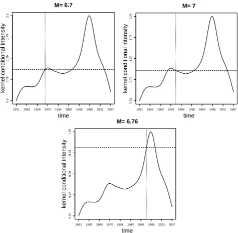
Fig. 5. Temporal kernel intensity conditioned to three big events,
0.0 0.5 1.0 1.5 2.0 2.5
172 174 176 178 180 −46
−44 −42 −40 −38 −36 −34
January, 1951
longitude
la
t
itude
0 2 4 6 8
172 174 176 178 180 −46
−44 −42 −40 −38 −36 −34
August, 1961
longitude
la
t
itude
0 2 4 6 8 10 12
172 174 176 178 180 −46
−44 −42 −40 −38 −36 −34
January, 1973
longitude
lati
t
ude
0 1 2 3 4 5 6
172 174 176 178 180 −46
−44 −42 −40 −38 −36 −34
June, 1984
longitude
la
t
itude
0 10 20 30 40
172 174 176 178 180 −46
−44 −42 −40 −38 −36 −34
November, 1995
longitude
la
t
itude
0 1 2 3 4 5 6
172 174 176 178 180 −46
−44 −42 −40 −38 −36 −34
March, 2007
longitude
lati
t
ude
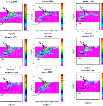
Fig. 6. Space-time-magnitude smoothed conditional intensity
func-tion forM=4.5 around a fixed point at six different times.
followed by a significant increasing of the activity. In partic-ular different cuts of magnitude have been effectuated, to see how the magnitude weighting may influence estimation re-sults and therefore these plots are generated by integrating the CIF over space and the specified magnitude regions. Al-though some tests might be useful, we observe significant differences between the plots in Fig. 4, that inform us about the complexity of the clustering features of events. Indeed it seems evident that time intensity estimation depends also on the magnitude of events, reflecting the not uniform behavior of aftershocks in time.
The clustering nature of events in time and space is also evident from Fig. 5. It represents the conditional intensity function estimated conditioning to three large events of the catalog withM=6.7, 7 and 6.8 occurred in three different dates and by integrating the CIF over space and magnitude domain. From these plots in correspondence of each main event we can observe a different behavior of their aftershocks sequences and their rate of activity. Indeed, the first main event is followed by an increasing clustered activity that
de-0.0 0.2 0.4 0.6 0.8 1.0 1.2
172 174 176 178 180 −46
−44 −42 −40 −38 −36 −34
January, 1951
longitude
lati
t
ude
0.0 0.5 1.0 1.5 2.0
172 174 176 178 180 −46
−44 −42 −40 −38 −36 −34
August, 1961
longitude
lati
t
ude
0.0 0.2 0.4 0.6 0.8 1.0 1.2
172 174 176 178 180 −46
−44 −42 −40 −38 −36 −34
January, 1973
longitude
lati
t
ude
0.0 0.5 1.0 1.5
172 174 176 178 180 −46
−44 −42 −40 −38 −36 −34
June, 1984
longitude
latitu
d
e
0 2 4 6 8 10
172 174 176 178 180 −46
−44 −42 −40 −38 −36 −34
November, 1995
longitude
lati
t
ude
0.0 0.5 1.0 1.5 2.0 2.5 3.0 3.5
172 174 176 178 180 −46
−44 −42 −40 −38 −36 −34
March, 2007
longitude
lati
t
ude
Fig. 7. Space-time-magnitude smoothed conditional intensity
func-tion forM=5.5 around a fixed point at six different times.
cays after a short period; this clustered activity comes before the second main event, followed by a decreasing activity pe-riod. A big rate of intensity is observed also after the third main event, with increasing values followed by a decreasing clustering effect.
0.000 0.001 0.002 0.003 0.004 0.005 0.006
172 174 176 178 180 −46
−44 −42 −40 −38 −36 −34
January, 1951
longitude
lati
t
ude
0.0 0.5 1.0 1.5
172 174 176 178 180 −46
−44 −42 −40 −38 −36 −34
August, 1961
longitude
lati
t
ude
0.00 0.01 0.02 0.03 0.04
172 174 176 178 180 −46
−44 −42 −40 −38 −36 −34
January, 1973
longitude
lati
t
ude
0.00 0.02 0.04 0.06 0.08 0.10 0.12 0.14
172 174 176 178 180 −46
−44 −42 −40 −38 −36 −34
June, 1984
longitude
lati
t
ude
0.0 0.2 0.4 0.6 0.8 1.0
172 174 176 178 180 −46
−44 −42 −40 −38 −36 −34
November, 1995
longitude
lati
t
ude
0.00 0.05 0.10 0.15
172 174 176 178 180 −46
−44 −42 −40 −38 −36 −34
March, 2007
longitude
lati
t
ude
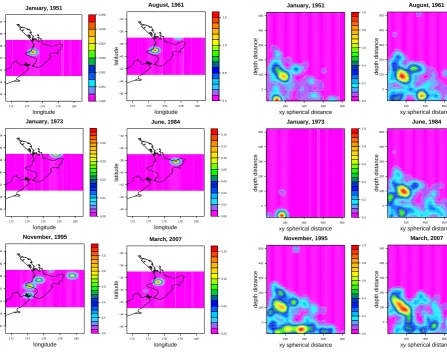
Fig. 8. Space-time-magnitude smoothed conditional intensity
func-tion forM=6.5 around a fixed point at six different times.
formula variation to compute distances on ellipsoids (Vin-centy, 1975). A variation of activity in time and space, from one part of the analyzed region to another, and between depths, is observed.
Although the provided analysis should be considered as just as a starting point for the comprehension of the com-plex mechanism of the observed seismicity in such different domains, we think that some interesting features have been highlighted. Indeed though the highly clustered seismicity identified by complex intensity function of the studied seis-mic area, the nonparametric approach makes possible a rea-sonable characterization of seismicity, since it does not con-strain the process to have predetermined properties.
The estimated model seems to follow adequately the seis-mic activity of the observed area, characterized by highly variable changes both in space and in time. The simple used approach provides a valid estimate of the conditional inten-sity in different domains that could be used for further inter-pretation according to the main object of interest. Indeed the activity rate is easily interpretable since the kernel approach
0.0 0.2 0.4 0.6 0.8 1.0
200 400 600 800 0
100 200 300 400 500
January, 1951
xy spherical distance
depth dis
t
ance
0.0 0.2 0.4 0.6 0.8 1.0
200 400 600 800 0
100 200 300 400 500
August, 1961
xy spherical distance
depth dis
t
ance
0.0 0.2 0.4 0.6 0.8 1.0
200 400 600 800 0
100 200 300 400 500
January, 1973
xy spherical distance
depth dis
t
ance
0.0 0.2 0.4 0.6 0.8 1.0
200 400 600 800 0
100 200 300 400 500
June, 1984
xy spherical distance
depth dis
t
ance
0.0 0.2 0.4 0.6 0.8 1.0
200 400 600 800 0
100 200 300 400 500
November, 1995
xy spherical distance
depth dis
t
ance
0.0 0.2 0.4 0.6 0.8 1.0
200 400 600 800 0
100 200 300 400 500
March, 2007
xy spherical distance
depth dis
t
ance
Fig. 9. 3-D space-time smoothed conditional intensity function
around a fixed point at six different times.
can be used to describe the variation in different domains and, because of its flexibility, it provides a good fitting to local space-time changes as just suggested by data.
5 Conclusions
Conditional intensity function as well as second order inten-sity provide useful indications of the strength and character of second order dependence effects between pairs of points at different separations of the analyzed domain.
In this paper a nonparametric estimate of conditional in-tensity for a multidimensional process is provided, using Gaussian kernel intensity estimators with constant bandwidth selection. Thus, both an estimate of this quantity and an eas-ily interpretable graphical summary of data are obtained.
For this reason, additional diagnostic analysis should be considered, although the high dimensionality could give some problems in finding a valid residual measures, as dis-cussed in Adelfio and Schoenberg (2009).
Acknowledgements. My sincerest gratitude to David Vere-Jones
for his very useful comments, but mostly for sharing his experience and kindness.
Edited by: G. Z¨oller
Reviewed by: E. Varini and another anonymous referee
References
Adelfio, G.: An analysis of earthquakes clustering based on a second-order diagnostic approach, in: Data Analysis and Clas-sification, Studies in ClasClas-sification, Data Analysis, and Knowl-edge Organization, edited by: Palumbo, F., Greenacre, M., and Lauro, C. N., Springer-Verlag, 309–317, 2010.
Adelfio, G. and Chiodi, M.: Second-order diagnostics for space-time point processes with application to seismic events, Environ-metrics, 20, 895–911, 2009.
Adelfio, G., Chiodi, M., De Luca, L., Luzio, D., and Vitale, M.: Southern-tyrrhenian seismicity in space-time-magnitude do-main, Ann. Geophys., 49(6), 1245–1257, 2006.
Adelfio, G. and Ogata, Y.: Hybrid kernel estimates of space-time earthquake occurrance rates using the etas model, Ann. I. Stat. Math., 62(1), 127–143, 2010.
Adelfio, G. and Schoenberg, F. P.: Point process diagnostics based on weighted second-order statistics and their asymptotic proper-ties, Ann. I. Stat. Math, 61(4), 929–948, 2009.
Cressie, N.: Statistics for spatial data, Wiley series in probability and mathematical statistics, 1991.
Daley, D. J. and Vere-Jones, D.: An introduction to the theory of point processes, 2nd edn., Springer-Verlag, New York, 2003. Doguwa, S. I.: On second order neighbourhood analysis of mapped
point patterns. Biometrical J., 4, 451–457, 1989.
Getis, A. and Franklin, J.: Second order neighbourhood analysis of mapped point patterns, Ecology, 68(3), 473–477, 1987. Grillenzoni, C.: Sequenzial kernel estimation of the conditional
in-tensity of nonstationary point processes, Statistical inference for stochastic processes, 9, 135–160, 2006.
Harte, D. and Vere-Jones, D.: Differences in coverage between the pde and new zealand local earthquake catalogues, New Zeal. J. Geol. Geop., 42(2), 237–253, 1999.
Ogata, Y.: Statistical models for earthquake occurrences and resid-ual analysis for point processes, J. Am. Stat. Assoc., 83(401), 9–27, 1988.
Ripley, B. D.: The second-order analysis of stationary point pro-cesses, J. Appl. Probab., 13(2), 255–266, 1976.
Schoenberg, F. P.: Testing Separability in Spatial-Temporal Marked Point Processes, Biometrics, 60, 471–481, 2004.
Silverman, B. W.: Density Estimation for Statistics and Data Anal-ysis, Chapman and Hall, London, 1986.
Utsu, T.: A statistical study on the occurrence of aftershocks, Geo-phys. Mag., 30, 521–605, 1961.
Vere-Jones, D.: Space-time correlations for microearthquakes: a pilot study, Adv. Appl. Probab., 10, 73–87, 1978.