Multiplicative cascade processes and information integration for predictive mapping

(1)

www.nonlin-processes-geophys.net/19/57/2012/ doi:10.5194/npg-19-57-2012

Nonlinear Processes

in Geophysics

Multiplicative cascade processes and information integration for

predictive mapping

Q. Cheng1,2

1_{State Key Lab of Geological Processes and Mineral Resources, China University of Geosciences, Beijing 100083,}

Wuhan 430074, China

2_{Department of Earth and Space Science and Engineering, Department of Geography, York University, Toronto,}

M3J1P3, Canada

Correspondence to: Q. Cheng ([email protected])

Received: 1 April 2010 – Revised: 5 December 2011 – Accepted: 22 December 2011 – Published: 11 January 2012

Abstract. This paper presents a new model proposed on the basis of multiplicative cascade process (MCP) theory for in-tegrating spatial information to be used for mineral resources prediction and environmental impact assessment. Probabil-ity of a spatial point event is defined as the probabilProbabil-ity that a small map calculating unit (map unit) randomly selected from a study area contains one or more points. The proba-bility that such unit randomly selected from a subarea with known spatial binary map patterns (evidential layers) con-tains one or more points is defined as the posterior point event probability. In this paper, processes of integrating multiple binary map patterns that divide the study area into smaller areas with updated posterior probabilities are viewed as mul-tiplicative cascade processes resulting in a new log-linear model for calculating conditional probabilities from the mul-tiple evidential input layers. The coefficients (weights) in-volved in this model measuring degree of spatial correlation between point event and the evidential layers are found to be associated with singularity indices involved in multifrac-tal modeling. It is demonstrated that the model is simple and easy to be implemented in comparison with the exist-ing weights of evidence model which is commonly applied in spatial decision modeling. In addition, the posterior prob-ability as the end product of a multiplicative cascade process can be used to describe multifractality and singularity which are useful properties for characterizing spatial distribution of predicted point events. A case study of tin mineral poten-tial mapping in the Gejiu mineral district in China is used to illustrate principles and use of the modeling process. Four binary layers: formation of limestone, buffer distance for in-tersections of three groups of faults, local and regional geo-chemical anomalies of elements As, Sn, Cu, Pb, Zn and Cd, were combined for mapping potential areas for occurrence of tin mineral deposits.

1 Introduction

Singular physical, chemical and biological processes can re-sult in anomalous energy release, mass accumulation or mat-ter concentration that, generally, are all confined to narrow intervals in space or time (Cheng, 2007a). Singularity is a property of non-linear natural processes, examples of which include cloud formation (Schertzer and Lovejoy, 1987), rain-fall (Veneziano, 2002), hurricanes (Sornette, 2004), flooding (Malamud et al., 1996; Cheng 2008), landslides (Malamud et al., 2004), forest fires (Malamud et al., 1996) and earth-quakes (Turcotte, 1997; Cheng et al., 1994a). The end prod-ucts of these non-linear processes can all be modeled as frac-tals or multifracfrac-tals.

(2)

58 Q. Cheng: Multiplicative cascade processes and information integration

geological features that control formation of mineral deposits can also be used to reduce the sizes of areas favorable for po-tential occurrences of undiscovered mineral deposits. For ex-ample, hydrothermal mineral deposits may occur around in-trusive rocks; thus certain buffer distance around intrusions can be delineated as favorable area for occurrence of min-eral deposits. Combining buffer zone around intrusions with other types of geological, geophysical and geochemical fac-tors such as fault structures that control distribution of min-eral deposits can further reduce the target areas for minmin-eral exploration. This paper aims to demonstrate that the concepts of multiplicative cascade processes (MCP) and singularities as the end products of MCP can be applied to model the processes of combining multiple geo-variables (evidence) to map potential areas for discovering new mineral deposits. A new model is developed to associate the posterior probabil-ity of a unit area containing mineral deposits and conditions observed in the unit area as multiple attributes. Using this model, posterior probabilities can be calculated from the in-put conditions and their associations with mineral deposits. These posterior probabilities can be considered as resulting from multiplicative cascade processes that may depict mul-tifractality and singularities which can be characterized by fractal and multifractal models.

2 Multifractal model and singularity distribution In order to show the potential association between multi-plicative cascade processes and information integration pro-cesses we first briefly introduce the concepts of multiplica-tive process, simple multifractal model and associated singu-larities. There are several formulisms for representing mul-tifractals; for example, deterministic and stochastic models. More information about various multifractal models can be found in Schertzer et al. (1997). Complete review of various multifractal models is out of the scope of this paper. Here we will only present some assumptions and relevant mathemat-ical notation for deterministic multifractals. Similar discus-sions can be partially applied to stochastic multifractal mod-els. Assume a measure,µ, defined in a small area of linear measuring size,εsatisfies

µ(ε)∝εα (1)

where∝stands for “proportional to” and αis the singular-ity index, also known as the coarse H¨older exponent; µis a function of scaleεwhich possesses isotropic scale invari-ance property so that the following ratio of logarithmic trans-formations ofµandεgives scale independent index whenε

approaches zero

α∝log[µ(ε)]

logε (2)

The values ofαusually vary in a finite interval [αmin,αmax]

for deterministic multifractals, but for other models, for ex-ample, whole family of the Universal Multifractal models

(Schertzer and Lovejoy, 1987) that include both theβ-model (Frisch et al., 1978) and the log-normal model (Yaglom, 1966), the bound of singularity might be infinite (Lovejoy and Schertzer, 2007). For some models the value of singu-larity can be negative and fractal dimension can be also neg-ative. According to the distribution of the value ofα, the entire mapped area can be classified into subsets or fractals, each of which possesses different singularity valueαi and,

accordingly, different fractal dimensions (f (αi)≤2). This is

the reason that the field ofµis described by the term “multi-fractality”. The fractal dimension functionf (α)and the sin-gularityαcan be estimated by various multifractal methods such as the method based on partition function (Halsey et al., 1986) and gliding box multifractal method (Cheng, 1999), just to name a few. For convenience of discussion, in this pa-per, we will use several terminologies pertaining to the multi-fractal model on the basis of partition function (Halsey et al., 1986), the entire study area can be partitioned into smaller subareas of equal sizeε×εand the measure of each such small area can be defined asµ(ε). Three functions: mass exponent function,τ (q), coarse H¨older exponent,α(q), and fractal spectrum function,f (α), can be introduced. They are associated according to the following relations (Halsey et al., 1986)

P_[

µ(ε)]q∝ετ (q)

α(q)=τ0(q)

f (α)=aq−τ (q)

(3)

whereqis the order of moment and the summation in the first equation is applied for all subareas of equal sizeε×εwith positive measureµ. From this formulation we can extract the following properties. Whenq=0 andα(0),f (α(0))= −τ(0), reaching the maximum value off (α)which corre-sponds to the box-counting fractal dimension. If the mea-sure covers the entire 2-D set, then the box-counting di-mension equals 2, otherwise it is less than 2; when q= 1 and α(1), f (α(1))=α(1)−τ(1). If the first moment

P

µ(ε)=constant, thenτ (1)=0 andf (α(1))=α(1). If we assume the numberNα(ε)of areas with sizeε×εcovering

the entire subset bearing the singularityα, and the fractal di-mensionf (α)of this subset are related by

Nα(ε)∝ε−f (α) (4)

The total measure of the subset can be expressed as

Nα(ε)µα(ε)∝ε−f (α)+α (5)

Since the total measure of the subset is less than the total measure of the entire set, the following relation must hold true:

α≥f (α) (6)

(3)

mapped area can be described by the fractal dimension spec-trum function f (α); this function reaching its maximum valuef (α(0))or the box-counting dimension of the support ofµatα(0). This implies that the majority of the area has measure characterized byα≈α(0), whereas areas with

val-uesα > α(0)orα < (0)are more irregular and with fractal

dimensionsf (α) < f (α(0)). Since the relation (6) holds true for allαandf (α), the singular areas with enrichment of the measure due toα <2 must have dimension f (α) <2 and those areas with measure depletion due toα >2 must have dimensionf (α)≤2; the equal sign applies only atα(0) (≥2).

3 Multiplicative cascade processes and multifractal distributions

The theory and concepts of multiplicative cascade processes play a fundamental role in explaining the generic conse-quence of scale invariant dynamics including turbulent in-termittency and other non-linear processes (Schertzer and Lovejoy 1985, 2007; Schertzer et al., 1997). There are sev-eral types of cascade models such as the log-normal model (Yaglom, 1966),α-model (Schertzer and Lovejoy, 1984) and p-model (Meneveau and Sreenivasan, 1987), to just name a few. A review of these models can be found in Schertzer et al. (1997). The model of de Wijs is a simple binomial mul-tiplicative cascade model for generating log-normal distribu-tion (de Wijs 1951). It became a multifractal model known as p-model (Meneveau and Sreenivasan, 1987). This model has been used to demonstrate generation of multifractal fields and their basic properties of singularities (Agterberg 2001, 2007a; Cheng, 2005; Ford and Blenkinsop, 2009). Other modifications to the model, for example, a cascade model with functional redistribution rate (Agterberg, 2007b) and a cascade model with variable partition processes (Cheng, 2005), are also available. A one-dimensional de Wijs’ cas-cade model is to be used in this paper for convenience in introducing the association between MCP and information integration processes. The de Wijs’ cascade model involves the partitioning of each unit segment into two sub-segments of equal size. The amount of measure (µ)in the unit seg-ment then can be written asd×µfor one half and (1-d)×µ

for the other half (0< d <1) so that total mass is preserved,

dµ+(1−d)µ=µ. The coefficient of dispersion,d, is in-dependent of segment size. At the beginning of the pro-cess, µ for the first segment can be set equal to unity. If

d >1/2, the maximum quantity of measure in small

seg-ment unit afternsubdivisions isµ=dn, and the minimum value isµ=(1−d)n; if d <1/2, the maximum and mini-mum values are switched. The general value of the measure in small segments after n subdivisions can be represented asµ=dk(1−d)n−k, where 0≤k≤n. The number of seg-ments with this value is

k n

. In a random cascade, larger and smaller values are assigned to segments using a discrete

random variable. The frequency distribution of the measure converges to a multifractal (Mandelbrot, 1989).

Letk/n=ξ, whereξ is a value with 0≤ξ≤1; then the value ofµ(ξ )= [dξ(1−d)1−ξ]n. The number of cells with

sizeεn=(1/2)n andµ(ξ )becomesN (εn)=

k n

. There-fore, the multifractal patterns generated by this cascade pro-cess have many local maxima and minima, with singularity expressed as follows (Feder, 1988; Halsey et al., 1986)

α= −ξln(d)+(1−ξ )ln(1−d)

ln2 (7a)

f (α)= −ξlnξ+(1−ξ )ln(1−ξ )

ln2 (7b)

The fractal dimension spectrumf (α)characterizes the distri-bution of measure with singularityα. The maximum and the minimum values ofαfrom Eq. (7a) areαmin= −log2(1−d)

andαmax= −log2[d], assumingd >1/2, therefore, the

gen-eral value of singularity becomes the combination of the max and min values ofα,α=ξ αmax+(1−ξ )αmin. It can be seen

that the range of singularityαis related to the choice ofd,

1αmax=αmax−αmin=log2[d/(1−d)]. As the valued

ap-proaches 1/2, the value range of singularity is reduced. If

d=1/2, then1αmax=0. According to the fractal

dimen-sion function, the sets with the maximum and the minimum singularity values have dimensionsf (α(0))=f (α(1))=0 and the areas with α(1/2)= −1/2log₂[d(1−d)] have di-mensionf (α(1/2))=1. It should be kept in mind that the relations (7a) and (7b) hold forp-model, and for other types of models the singularity range can be unbounded.

4 Information integration processes for mapping mineral potential

(4)

1

31

E

~

1

E

1 1

E

~

Fig. 1 Schematic diagram showing location of mineral deposits (D) shown as stars are highly associated with igneous batholith . Relatively fewer mineral deposits are located outside of batholith labeled as

1

E

1

E~.

Fig. 1. Schematic diagram showing location of mineral deposits

(D) shown as stars are highly associated with igneous batholithE1. Relatively fewer mineral deposits are located outside of batholith labeled as_E˜

1.

Successive overlay of evidential layers progressively parti-tions the study area into smaller sub-areas with updated pos-terior probability of containing points per unit area. In this paper it will be shown that the process of integrating layers of information has similarities with the multiplicative cascade process introduced previously. For convenience without loss of generality, we will use binary evidential layers as an ex-ample to illustrate this relationship. We need to define some notations as follows.

Let T represent a study area (a 2-D set); {Ei,E˜i}(i=

1,2,...,n)represent series of maps of mutually exclusive

bi-nary patterns, Ei and E˜i, Ei∩ ˜Ei =φ, and Ei∪ ˜Ei=T,

where “∩” and “∪” stand for intersection and union, respec-tively. From now on an intersection of sets appears like a product of them. Superimposing these binary patterns di-vides the study areaT into smaller sub-areas. For example, four possible intersections:EiEj, EiE˜j,E˜iEj,E˜iE˜jcan be

formed when two maps,{Ei,E˜i}and{Ej,E˜j}are combined.

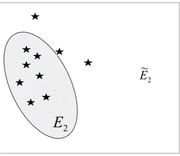
To illustrate the definitions and binary patterns and their as-sociations with mineral deposits (D), several schematic dia-grams are provided in Figs. 1 to 3 to present two binary maps, igneous batholith and alteration zone, considered as control-ling factors for the occurrence of hydrothermal mineral de-positsD. Each of the two binary maps divides the study area into two sub-classes: favorable areas (E) and unfavorable ar-eas (E)˜ for formation of mineral deposits, E∪ ˜E=T and

EE˜=8. In this artificial example, 10 discovered mineral deposits are labeled as dots on the map and 60 % of them are located on the igneous batholith (E1)and 40 % off the

igneous batholith (E˜1), 70 % of points on alteration zone

(E2)and 30 % off alteration zone (E˜2). The binary patterns

are defined according to certain geological features, some of them with natural boundaries such as contacts between rock formations, while other patterns could be defined as man-made features with thresholds such as geological anomalies with concentration values above a certain cutoff value.

2

E

~

32

2

E

2

E

~

E

₂

Fig. 2 Schematic diagram showing location of mineral deposits (D) shown as stars are highly associated with alteration zone labeled as . Relatively fewer mineral deposits are located outside of alternation

2

E

zone labeled asE2

~_.

Fig. 2. Schematic diagram showing location of mineral deposits (D) shown as stars are highly associated with alteration zone la-beled asE2. Relatively fewer mineral deposits are located outside of alternation zone labeled as_E˜

2.

2

1

E

~

E

~

2 1

E

~

E

2 1

E

~

2

1

E

2

1

E

~

E

~

2 1

E

~

E

2 1

E

~

2

1

E

Fig. 3 Schematic diagram showing mineral deposits (D) shown as stars and two binary maps partitioning the study area into four subareas labeled as

2 1 2 1 2 1 EE

~ , E~ E , E

E 1E2

~ E~

and , respectively.

33

Fig. 3. Schematic diagram showing mineral deposits (D) shown as stars and two binary maps partitioning the study area into four subareas labeled asE1E2,E1E˜2,E˜1E2andE˜1E˜2, respectively.

In order to associate point events (e.g., mineral deposits in a mineral district) with these binary maps, we define prob-abilities and conditional probprob-abilities as follows. Assume a small map unit is defined (for example pixel of image) so that each point ofDoccupies only one map unit, then the number of map units occupied by mineral deposits and by map pat-ternsEi andE˜i can be used to estimate the probabilities and

conditional probabilities. For example, the prior probability,

P[D], of a randomly selected map unit containing a mineral deposit can be estimated by the number of map units occu-pied by mineral deposits,n(D), divided by the total number of map units occupied byT,n(T )as

P[D] =n(D)

(5)

We denote prior probability of mineral deposits asP[D]. Similarly, we can define the probabilities of eventsEi,Ej

and their intersections. The conditional probability of D

given condition of patterns Ei and E˜i can be accordingly

defined and denoted asP[D|Ei] andP[D| ˜Ei], respectively.

These conditional probabilities can be estimated as the ratio of the number of map units occupied both by mineral de-posits and by patternEi orE˜i over the total number of map

units occupied byEiorE˜i, respectively

P[D|Ei] =n(DE_n(E_i₎i)

P[D| ˜Ei] =n(D ˜ Ei)

n(_E˜

i)

(9)

wheren(DE)andn(DE)˜ represent the number of map units occupied both by mineral deposits and by pattern Ei or

˜

Ei, respectively. IfP[D] is considered as the initial

mea-sure of mineral deposits in the entire area, each addition of an evidential layer of binary pattern (Ei andE˜i)will

pro-duce one sub-area (favorable area) with a conditional (pos-terior) probability that is increased (enhanced),P[D|Ei]>

P[D], and another sub-area (unfavorable areas) with a con-ditional (posterior) probability that is decreased (depleted),

P[D| ˜Ei]< P[D].

Similarly, we can define probabilities and conditional probabilities forD and any possible multiple intersections of patterns, for example,

P[D|E₁∗E₂∗...E∗_n] (10)

whereE∗₁E₂∗...E_n∗(E_i∗=EiorE˜i)is an intersection ofn

pat-terns. In the following sections we will discuss properties of the process of integrating map patterns.

In order to ensure the process of integration of binary terns can reduce the areas with unique intersection of pat-terns, we make the further assumption: all probabilities and conditional probabilities are positive and all patterns are con-ditionally independent from each other with respect toD,

P[D]>0, P[Ei]>0, P[ ˜Ei]>0 (11a)

P[Ei|D]>0, P[ ˜Ei|D]>0 (11b)

P[E₁∗E₂∗...E_n∗|D] =P[E∗₁|D]P[E₂∗|D]...P[E_n∗|D] (11c) The main goal of information integration processes is to combine multiple binary map patterns to divide the entire area into smaller areas on the basis of unique intersections of patternsP[E₁∗E₂∗...E_n∗] and to calculate the correspond-ing posterior probabilitiesP[D|E₁∗E₂∗...E_n∗]. The posterior probability map shows areas with high or low probabilities of having mineral deposits and this type of information is useful for mineral exploration. In the following sections we will investigate information integration model from the point of view of cascade processes.

From the conditional independency condition (11c) we can derive the following relation between conditional proba-bility and the probabilities of patterns

2lnP[E₁∗E₂∗...E_n∗|D] =

α(E₁∗)lnP[E₁∗] +α(E₂∗)lnP[E∗₂] +...+α(E_n∗)lnP[E∗_n] 2lnP[D|E₁∗E₂∗...E∗_n] =

P[D] P[E∗₁E∗₂...E∗

n]

α E∗₁lnP[E∗₁] +α E₂∗lnP[E∗2]+ ....+α E_n∗lnP[E_n∗]

(12)

where each coefficient can be expressed as

α(E∗_i)=α(Ei)orα(E˜i)

α(Ei)=2ln_lnP_P[E_[Ei|D]

i]

α(E˜i)=2ln_lnP[ ˜Ei|D] P[ ˜Ei]

(13)

This form (12) is a log-linear model associating the con-ditional probabilities P[D|E₁∗E∗₂...E_n∗] and each probabil-ity of pattern P[E_i∗]. Therefore, the form (12) with coef-ficients (13) provides a new model for calculating posterior probability. This model will be compared with weights of evidence model in Sect. 5.

5 Information integration processes and multifractal distribution

5.1 Conditional independent cascade processes

In order to show the similarity between the information inte-gration model discussed in Sect. 3 and generalized binomial cascade processes, the simple one-dimensional de Wijs’s multiplicative cascade processes introduced in Sect. 2 will be compared with each other. The de Wijs’s cascade pro-cesses involve binary partitioning of each unit segment into two equal segments in each generation. For random parti-tioning, knowledge of the details of the partition is not re-quired, so we can use probability notation to represent the processes. Comparing the notations used for information in-tegration with those introduced in de Wijs’ model, we can define a measure as the proportion of map units containing

Das well as measures for the proportions of map units onD

and the various patternsEiusing joint probabilities. Suppose

initial measure in the entire area is defined as

µ=n(D)

n(T ) =P[D] (14)

and measures on each pair of subareas for patternsEi andE˜i

after a partition as

µ[Ei] =P[D Ei]

µ[ ˜Ei] =P[DE˜i]

(6)

Similarly, we consider the ratio of the linear size of setE∗

and the size of the entire area as the measuring scale

ε2 =n(E

∗₎

n(T ) =P[E

∗_] ₍₁₆₎

The dispersion coefficient di and 1−di as proportions of

measures redistributed inEi andE˜i involved in the partition

can be expressed as

di=µ[E_µ[D]i]=P[Ei|D]

1−di=µ[ ˜_µ[D]Ei]=P[ ˜Ei|D]

(17)

According to the definitions of the probabilities of the events

P[E₁∗E₂∗...E_n∗], the area sizes of these events (number of map units containing a specific combination of patterns) are pro-portional to the probabilities

n(E₁∗E₂∗...E_n∗)=n(T )P[E₁∗E₂∗...E_n∗] (18)

wheren(T ) is the total number of map units covering the entire study area. Due to the property that every further par-tition will reduce the total area into two subareas, the size of the partitioned subareas generally decreases with increase of numbers of partitions. Further the positive probability re-quirement and conditional independency assumption given in Eq. (11a to c) ensure the following monotonically de-scending relationship

P[E₁∗E₂∗...E_k−∗ ₁]> P[E₁∗E₂∗...E∗_k] (19)

Relation (19) must be true because, otherwise, if

P[E₁∗E₂∗...E_k−∗ ₁] =P[E₁∗E₂∗...Ek] it would follow that

P[E₁∗E₂∗...E˜k] = P[E∗₁E₂∗...E_k−∗ ₁] − P[E₁∗E₂∗...Ek] = 0,

and, therefore, P[E∗₁E₂∗...E˜k|D] = 0, according to the

conditional independency assumption (11c) it must exist one evidence so that P[E_i∗|D] =0, which would violate the condition (11a to b). The relation (19) indicates that the sizes of the subareas defined by the intersection of patternsE₁∗E₂∗...E_n∗monotonically decrease with increasing number of partitions. Keep in mind that without conditional independency assumption amongE₁∗E∗₂...E_n∗ (Eq. 11c) the strict monotonic relation (19) may not be held and some subareas delineated by intersection of sets may not approach to zero. In comparison with the relations (1) and (2), the end product may show multifractal distribution with singularities expressed as

P[DE_k∗ 1E

∗ k2...E

∗

kn] ∝P[E

∗ k1E

∗ k2...E

∗ kn]

α/2 P[D|E_k∗

1E

∗ k2...E

∗

kn] ∝P[E

∗ k1E

∗ k2...E

∗ kn]

α/2−1 (20)

The form (20) may be not valid in general but its validity in some special cases will be proved as to be discussed in the next section. If the form (20) holds true, then the singularity index valueαdetermines the rate of change of the posterior probability when the number of partitions is increased with reduction of areas proportioned toP[E∗₁E∗₂...E_n∗]in three sit-uations:

1. if and only ifα >2, thenP[D|E₁∗E∗₂...E_n∗]decreases; 2. if and only ifα <2, thenP[D|E₁∗E∗₂...E_n∗]increases; 3. if and only if α=2, then P[D|E∗₁E₂∗...E_n∗] is

un-changed.

These three properties imply that the posterior probability in-creases when singularity indexα <2, decreases whenα >2 and remains unchanged whenα=2.

5.2 Independent and constant cascade processes To demonstrate the analogies between the de Wijs model and the pattern partitions, we will make following assumptions in addition to the conditional independency assumption (11c):

(1) All partitions are independent from each other

P[E₁∗E₂∗...E_n∗] =P[E₁∗]P[E₂∗]...P[E_n∗] (21) (2) All binary events have the same probability and the same conditional probability

P[Ei] =P[E],P[ ˜Ei] =P[ ˜E]

d=P[Ei|D] =P[E|D],1−d=P[ ˜Ei|D] =P[ ˜E|D] (22)

Now we can derive the probability ofDon the subarea with

k occurrences ofE andn−k times E˜ when combining n binary patternsE∗₁E₂∗...E_n∗as

P[DEkE˜n−k] =P[D]P[EkE˜n−k|D] =

P[D](P[E|D])kP[ ˜E|D] n−k

=P[D]dk(1−d)n−k (23)

Accordingly, the probability ofP[EkE˜n−k]can be written as

P[EkE˜n−k] =(P[E])kP[ ˜E]n−k (24)

Therefore, the quantity ofDon subareas defined withktimes

Eandn−ktimesE˜can be written asµ=P[D]dk(1−d)n−k

and the number of such subareas asN=

k n

. Letk/n=

ξ and considering the size of subareas is proportional to

P[EkE˜n−k]; then

α=2ξlnP[E|D] +(1−ξ )lnP[ ˜E|D]

ξlnP[E] +(1−ξ )lnP[ ˜E] (25a)

f (α) =2 ξlnξ+(1−ξ )ln(1−ξ )

ξlnP[E] +(1−ξ )lnP[ ˜E] (25b) According to relation (25a), we obtain the maximum and minimum singularities as

α(E)=2lnP[E|D]/lnP[E]

(7)

and further the following forms

P[E|D] =P[E]α(E)/2

P[ ˜E|D] =P[ ˜E]α(E)/˜ 2

P[D|E] =P[D]P[E]α(E)/2−1

P[D| ˜E] =P[D]P[ ˜E]α(E)/˜ 2−1

(27)

The Eq. (27) is a special form of Eq. (20). Therefore, from Eqs. (25a) and (26) it follows that the general value of singu-larity is a linear combination of the valuesα(E)andα(E)˜ . If we further assumeP[E] =P[ ˜E] =0.5, then relations (25a) and (25b) become the same relations as shown in Eq. (7a) and (7b). In this special case each partition divides the previously divided subareas into two equal subareas and the dispersion coefficientd is independent of the partitioning.

6 Weights of evidence model for information integration in predictive mapping

Several methods have been developed for combining mul-tiple layers of evidence (E₁∗E₂∗...E_n∗)to map the posterior probabilityP[D|E₁∗E∗₂...E_n∗]for prediction of mineral de-posits. The weights of evidence method is one of the most commonly used methods for integration of evidential lay-ers for predictive purposes (Bonham-Carter et al., 1988; Agterberg 1989a, b; Agterberg and Bonham-Carter, 1990; Bonham-Carter, 1994). Under the assumption of conditional independency Eq. (11a to c) the weights of evidence method gives the following logistic model for calculating posterior probability

P[D|E₁∗E₂∗...E∗_n] = 1

1+e−(W0+WE∗1+WE ∗ 2+...+WE

∗

n)

(28)

whereW0andWE∗are weights as shown below

Wo=ln

_P_[_D_]

P[ ˜D]

WEi=ln

P[Ei|D]

P[Ei| ˜D]

,W_E˜

i=ln

P[ ˜Ei|D]

P[ ˜Ei| ˜D] !

(29)

In order to compare the logistic model (28) and the new model (12), we will show the association between the weightsWE andW_E˜ shown in Eq. (29) and the singularity

indices(E)andα(E)˜ in Eq. (13).

We can see from their definitions that the main differences betweenWE, W_E˜ andα(E), α(E)˜ are that the former

in-volveP[E| ˜D],P[ ˜E| ˜D]but the latter involve onlyP[E]and

P[ ˜E]. Since the latter do not involve any associations of pat-terns and the complementary eventD˜, it is relatively easier to calculate the singularity indicesα(E)andα(E)˜ than the weightsWE andW_E˜. Otherwise, these two types of indices

carry the same type of information about the association of

patternsE,_E˜ _{and event}_D_{as can be concluded from the} fol-lowing properties:

(1)WE=0↔α(E)=2,W_E˜=0↔α(E)˜ =2;

(2)WE>0↔α(E) <2,W_E˜>0↔α(E) <˜ 2;

(3)WE<0↔α(E) >2,W_E˜<0↔α(E) >˜ 2;

We just need to prove the first property (1) and the other two properties can be proved similarly. For example, if

WE=0, thenP[E|D] =P[E| ˜D], which leads toP[E|D] =

P[E] so that α(E)=2. On the other hand, if α(E)= 2, then P[E|D] =P[E] so that P[ED] =P[E]P[D] and further, P[ED˜] =P[E] −P[ED] =P[E] −P[E]P[D] =

P[E]P[ ˜D], therefore,P[E| ˜D] =P[E] and WE=0. This

proves the first property (1) implying thatDandEare in-dependent. The other two properties correspond to positive correlation between D and E, and P[E|D]> P[E| ˜D] or

P[E|D]> P[E]and negative correlation betweenDandE,

P[E|D]< P[E| ˜D]orP[E|D]< P[E], respectively.

7 Application of information integration processes in mineral resources assessment

7.1 Study area and data

(8)

34 1

Fig. 4 Simplified geology of Gejiu mineral district. Pink polygons distributed in the center of the study area stand for Gejiu Batholith of felsic intrusions, yellow polygons for Gejiu formation of limestone, black lines represent faults, white areas for other sedimentary rocks, and dots for Sn mineral deposits.

Fig. 4. Simplified geology of Gejiu mineral district. Pink polygons

distributed in the center of the study area stand for Gejiu Batholith of felsic intrusions, yellow polygons for Gejiu formation of lime-stone, black lines represent faults, white areas for other sedimentary rocks, and dots for Sn mineral deposits.

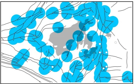
Fig. 5 Faults systems. Black lines represent faults. Blue circles stand for 6km buffer zones around intersections of three fault systems.

35

Fig. 5. Faults systems. Black lines represent faults. Blue circles

stand for 6 km buffer zones around intersections of three fault sys-tems.

In the author’s previous studies, four factors related to mineralization were identified according to a hydrothermal mineral deposit genesis model; accordingly, four binary lay-ers were constructed using various GIS and spatial analysis techniques. These four layers are: (1) Gejiu formation of carbonates (Gf) (Fig. 4); (2) the 6 km buffer zone around the intersections of three groups of faults (Bf) (Fig. 5); (3) lo-cal geochemilo-cal anomalies (La) delineated from concentra-tion values of the elements Sn, As, Zn, Pb, Cu and Cd in stream sediment samples (Fig. 6); and (4) regional geochem-ical anomalies (Ra) delineated from values of Sn, As, Zn, Pb, Cu and Cd in stream sediment samples (Fig. 7). More detailed information about the definition of the four binary layers can be found in Cheng et al. (2009). This paper will use these four binary layers to calculate the posterior proba-bility map according to relation (12) and to demonstrate the processes of combining layers and the singularities of the created posterior probability map.

Fig. 6 Local geochemical anomalies extracted from concentration val elements Sn, As, Cu, Pb, Zn and Cd. First singularity index was ca the concentration values

ues of lculated from of each element and these singularity maps were combined by means of principal component analysis. The patterns in red are the binary patterns created from the score on the first component. Details can be found in Cheng et al. (2009).

36

Fig. 6. Local geochemical anomalies extracted from concentration

valelements Sn, As, Cu, Pb, Zn and Cd. First singularity index was cathe concentration valuesues of lculated from of each element and these singularity maps were combined by means of principal component analysis. The patterns in red are the binary patterns cre-ated from the score on the first component. Details can be found in Cheng et al. (2009).

7.2 Results

Each information layer to be combined (binary patterns of which are shown in Figs. 4 through 7) divides the study area into two subclasses of reduced area that represent favorable and unfavorable regions for predicting mineral deposits. If we define a square of size 1×1 km2as the measuring unit, the total study area occupies about 1688 units. There are a to-tal of 11 units occupied by Sn mineral deposits, from which the prior probability of a randomly chosen square from the area containing mineral deposits can be estimated asP[D] = 0.0065. Similarly, one can calculate the number of units oc-cupied by binary patterns and the number ococ-cupied by both binary patterns and mineral deposits. Table 1 gives the results obtained from the four binary maps Gf, Bf, La and Ra. The second and third columns in Table 1 show the areas (number of units) of the favorable patterns of each binary map and the numbers of mineral deposits occurring in each of the patterns (# points on pattern). From these two columns, one can cal-culate the probability of patterns for each of the four binary maps; for example, probability of Geijiu formationP[Gf]= 747/1688=0.44 andP[Gf]˜ =1−P[Gf]=0.56, represent-ing the probabilities that patterns exist on the Gejiu forma-tion and the complementary event (on other rock types). One can also calculate the probability that a unit area of a given binary pattern contains mineral deposits, for example,

(9)

Table 1. Statistics obtained from each of the four layers of binary maps.

Area # WE s(WE) W_E˜ s(W_E˜) C s(C) t-value α α(E)˜ 1α

points αmax−αmin

Rock Type (Gf) 747 7 0.35 0.38 −0.40 0.49 0.75 0.63 1.2 1.11 3.46 2.35

Dist. to Inter. (Bf) 515 6.4 0.66 0.40 −0.52 0.47 1.18 0.61 1.92 0.91 4.79 3.88

Geochem. I (La) 188 8 1.91 0.36 −1.19 0.58 3.10 0.68 4.54 0.29 22.01 21.72

Geochem. II (Ra) 309 6 1.12 0.41 −0.61 0.45 1.73 0.61 2.84 0.71 7.8 7.09

Fig. 7 Regional geochemical anomalies extracted by applying S-A filtering to the scores calculated from the first principal component

fractal derived from logarithmic transformed concentration values of elements Sn, As, Cu, Pb, Zn and Cd. The patterns in red are the binary patterns created from the decomposed patterns by means of S-A method. Details can be found in Cheng et al. (2009).

37

Fig. 7. Regional geochemical anomalies extracted by applying S-A

filtering to the scores calculated from the first principal component fractal derived from logarithmic transformed concentration values of elements Sn, As, Cu, Pb, Zn and Cd. The patterns in red are the binary patterns created from the decomposed patterns by means of S-A method. Details can be found in Cheng et al. (2009).

other binary patterns are similarly calculated and are shown in Table 1.

The other values shown in Table 1 are statistics used in the weights of evidence method. Value ofs(W )stands for standard deviation ofW and t-value is for Student’s statistic value of the contrast of weightsC=WE−W_E˜. The results in

Table 1 show that the four binary maps are all positively cor-related withD. Among them, the local geochemical anoma-lies (La) show the highest contrast of weights with t-value (Student’s statistic)t=4.54 (for calculation ofW,s(W ), and t-values ofC, see Bonham-Carter, 1994). The values of sin-gularity indicesα(E)=0.29<2 andα(E)˜ =22.01>2 also imply that the singularity related to pattern La is strong. In general, the ranges of singularity 1α=αmax–αmin are all

positive which implies that all four layers are positively as-sociated withD. In addition, the ranks of the ranges of sin-gularity 1α are similar to the ranks of the t-values which implies that the range of singularity can be used as a statis-tic measuring the degree of correlation betweenD and the patterns. Since all four map layers are associated with the location ofD, these four layers must be combined in order to create a posterior probability map that shows the best areas

38 1

2

3

4

5

6

7

8

Fig. 8 Posterior probability map created by means of weights of evidence method applied to the four evidential layers in Figs. 4 to 7.

Post Prob

Fig. 8. Posterior probability map created by means of weights of

evidence method applied to the four evidential layers in Figs. 4 to 7.

for occurrences of mineral deposits. Using model (12), four layers of binary maps were combined; the posterior proba-bility map that emerged is shown in Fig. 8. The areas with high posterior probability values contain most of the known mineral deposits; some areas with high posterior probabili-ties in which mineral deposits have not yet been found can be considered target areas for further exploration.

(10)

39 1

y = 0.0009x-1.4653

R2_{= 0.9707}

0.00 0.00 0.01 0.10 1.00

0.01 0.10 1.00

LnP[G]

LnP[D|G]

Fig. 9 Relationship between posterior probability P[D|G] and the probability of the area (G) with cutoff value of posterior probability. Fig. 9. Relationship between posterior probabilityP[D|G]and the

probability of the area (G) with cutoff value of posterior probability.

mid-point value of−1.4354 and each class interval equal to 0.299. Cumulative frequencies of map units in each class were calculated and these values are plotted in Fig. 9. In Fig. 9 the posterior probability corresponding to the mid-point value of each class, denoted asP[D|G] and the prob-ability of the cumulative number of map units occupying these classes, denoted asP[G], are plotted. The result gener-ally shows a power-law relationship between the cumulative area and the mid-point class value of posterior probability,

P[D|G] =0.0009P[G]−1.4653. Since the posterior probabil-ityP[D|G] is the value at boundary ofG, the average poste-rior probability inGshould also follow power-law relations withP[G]with exponent−0.4653 which gives the singu-larityα/2=0.4653 andα=1.08<2 implying a general en-richment of posterior probability at the peaks when the size of areaGdecreases.

8 Conclusions and discussion

Multiplicative cascade processes are non-linear processes commonly observed in geoscience that can create end prod-ucts that follow multifractal distribution with multi-scale sin-gularities. Singularity is a natural property of mineralization, which involves enrichment and depletion of ore and associ-ated elements in the Earth’s crust as well as in other relevant secondary media such as tills, soils, lake and stream sedi-ments, humus and vegetation surrounding mineral deposits. Mapping such singularities is an effective way to delineate areas favorable for occurrence of mineral deposits and esti-mate the likelihood of the presence of undiscovered mineral resources in a given area.

To support decision-making and to map areas for predic-tion of mineral deposits, multiple layers of informapredic-tion that are positively associated with the location of mineral deposits must often be combined. This information integration pro-cess can be considered as a type of multiplicative cascade process that updates the posterior probability by combining evidence layers. The model proposed in this paper provides an alternative log-linear relationship associating conditional

probability of points and evidence layers with singularity in-dices as coefficients, which quantify degree of spatial corre-lation between binary patterns and location point events (e.g., mineral deposits). This feature is important for three reasons: first, it links the concepts and methods of multifractal model-ing developed in nonlinear processes in geophysics and infor-mation integration modeling commonly employed for spatial decision support. Secondly, the newly developed log-linear model can not only be used as an alternative model for formation integration but also provides relatively simpler in-dices in comparison with the weights of evidence method. This is because the singularity indices involved in the new model do not require calculation of probabilities and con-ditional probabilities related to complementary point events. In addition, as the end product of a multiplicative cascade process, the posterior probability may possess multifractality with singularities that can be further investigated for char-acterization of the spatial distribution of the point events. Moreover, the results and formulation developed in the cur-rent research might be useful for further study of more gen-eralized multiplicative cascade processes. It must be kept in mind that a large number of evidential layers are usually needed to create posterior probability maps that are represen-tative of multifractal fields. However, when the number of bi-nary patterns increases, the dependency among the patterns and between patterns and point events becomes inevitable. Therefore, a more general model overcoming these depen-dency problems has to be developed.

Acknowledgements. Sincere thanks are due to the editor D. Schertzer and two anonymous reviewers for providing constructive comments which have significantly improved the paper. The author thanks Frits Agterberg for reading this manuscript and providing constructive comments. The research was financially supported by a High-Tech Research and Devel-opment Grant (2009AA06Z110) by the Ministry of Science and Technology of China, and Grants from Ministry of Education of China (No. IRT0755).

Edited by: D. Schertzer

Reviewed by: two anonymous referees

References

Agterberg, F. P.: Computer programs for exploration, Science, 245, 76–81, 1989a.

Agterberg, F. P.: Systematic approach to dealing with uncertainty of geoscience information in mineral exploration, in: Application of Computers and Operations in the mineral industry, edited by: Weiss, A., Proc. 21st APCOM Symp., Las Vegas, Nevada, Col-orado Society of Mining Engineers, Littleton, 165–178, 1989b. Agterberg, F. P.: Multifractal modeling of the sizes and grades of

giant and supergiant deposits, Int. Geol. Review, 37, 1–8, 1995. Agterberg, F. P.: Multifractal simulation of geochemical map

(11)

Agterberg, F. P.: New applications of the model of de Wijs in re-gional geochemistry, Math. Geol., 39, 1–26, 2007a.

Agterberg, F. P.: Mixtures of multiplicative cascade models in geochemistry, Nonlin. Processes Geophys., 14, 201–209, doi:10.5194/npg-14-201-2007, 2007b.

Agterberg, F. P. and Bonham-Carter, G. F.: Deriving weights of evi-dence from geoscience contour maps for prediction of discrete events, Proc. 22nd APCOM Symp. (Berlin, Germany), Tech. Univ. Berlin, 2, 381–396, 1990.

Blenkinsop, T. G.: The Fractal Distribution of Gold Deposits, in: Fractals and Dynamic Systems in Geoscience, edited by: Kruhl, J. H., Springer-Verlag, 247–258, 1994.

Bonham-Carter, G. F.: Geographic Information Systems for Geo-scientists: Modelling with GIS, Pergamon, Oxford, 398 pp., 1994.

Bonham-Carter, G. F., Agterberg, F. P., and Wright, D. F.: Integra-tion of geological data sets for gold exploraIntegra-tion in Nova Scotia, Photogr. Eng. Remote Sens., 54, 1585–1592, 1988.

Carlson, C. A.: Spatial distribution of ore deposits, Geology, 19, 111–114, 1991.

Cheng, Q.: The gliding box method for multifractal modeling, Comput. Geosci., 25, 1073–1079, 1999.

Cheng, Q.: Fractal and multifractal modeling of hydrothermal min-eral deposit spectrum: application to gold deposits in the Abitibi Area, Canada. J. China Univ. of Geosci., 14, 199–206, 2003. Cheng, Q.: Multifractal distribution of eigenvalues and eigenvectors

from 2-D multiplicative cascade multifractal fields, Math. Geol., 37, 915–927, 2005.

Cheng, Q.: Mapping singularities with stream sediment geochem-ical data for prediction of undiscovered mineral deposits in Gejiu, Yunnan Province, China, Ore Geol. Reviews, 32, 314– 324, 2007a.

Cheng, Q.: Multifractal imaging filtering and decomposition meth-ods in space, Fourier frequency, and eigen domains, Nonlin. Pro-cesses Geophys., 14, 293–303, doi:10.5194/npg-14-293-2007, 2007b.

Cheng, Q.: Non-linear theory and power-law models for informa-tion integrainforma-tion and mineral resources quantitative assessments, Math. Geosci., 40, 503–532, 2008.

Cheng, Q. and Agterberg, F. P.: Multifractal modeling and spatial statistics, Math. Geol., 28, 1–16, 1996.

Cheng, Q. and Agterberg, F. P.: Fuzzy weights of evidence method and its application in mineral potential mapping, Nat. Res. Res., 8, 27–35. 1999.

Cheng, Q. and Agterberg, F. P.: Singularity analysis of ore-mineral and toxic trace elements in stream sediments, Comput. Geosci., 35, 234–244, 2009.

Cheng, Q., Bonham Carter, G. F., Agterberg, F. P., and Wright, D. F.: Fractal modeling in the geosciences and implementation with GIS, in: Proc of the 6th Canadian Conference on GIS, Ottawa, June 6, 10, 1, 565–577, 1994a.

Cheng, Q., Agterberg, F. P., and Ballantyne, S. B.: The separation of geochemical anomalies from background by fractal methods, J. Explor. Geochem., 51, 109–130, 1994b.

Cheng, Q., Zhao, P., Zhang, S., Xia, Q., Chen, Z., Chen, J., Xu, D., and Wang, W.: Application of singularity in mineral deposit pre-diction in Gejiu district: Information integration and delineation of target areas, Earth Science, 34, 243–252, 2009 (in Chinese with English abstract).

de Wijs, H. J.: Statistics of ore distribution, part I, Geologie Mijn-bouw, 13, 365–375, 1951.

Feder, J.: Fractals, Plenum Press, New York, 283 pp., 1988. Ford, A. and Blenkinsop, T. G.: An expanded de Wijs model for

multifractal analysis of mineral production data, Mineral De-posita, 44, 233–240, 2009.

Frisch, U., Sulem, P. L., and Nelkin, M.: A simple dynamical model of intermittency in fully develop turbulence, J. Fluid Mech., 87, 719–724, 1978.

Halsey, T. C., Jensen, M. H., Kadanoff, L. P., Procaccia, I., and Shraiman, B.: Fractal measures and their singularities: the char-acterization of strange sets, Phys. Rev. A, 33, 1141–1151, 1986. Hronsky, J. M. A: Self-organized systems and ore formation: the key to spatially-predictive targeting?, Proceedings of the Tenth Biennial SGA Meeting, Townsville 2009, 19–21, 2009. Lovejoy, S. and Schertzer, D.: Scaling and multifractal fields in

the solid earth and topography, Nonlin. Processes Geophys., 14, 465–502, doi:10.5194/npg-14-465-2007, 2007.

Malamud, B. D., Turcotte, D. L., and Barton, C. C.: The 1993 Mis-sissippi river flood: a one hundred or a one thousand year event?, Environ. Eng. Geosci., II, 479–486, 1996.

Malamud, B. D., Turcotte, D. L., Guzzetti, F., and Reichenbach, P.: Landslide inventories and their statistical properties, Earth Surf. Proc. Land., 29, 687–711, 2004.

Mandelbrot, B. B.: Multifractal measures, especially for the geo-physicist, Pure Appl. Geophys., 131, 5–42, 1989.

Meneveau, C. and Sreenivasan, K. R.: Simple multifractal cascade model for fully developed turbulence, Phys. Rev. Lett., 59, 1424– 1427, 1987.

Qing, D., Tan, S., and Fan, Z.: Geotectonic evolution and tin-polymetallic metallogenesis in Gejiu-Dachang area, J. Mineral., 24, 118–123, 2004 (in Chinese with English Abstract).

Raines, G: Are fractal dimensions of the spatial distribution of min-eral deposits meaningful?, Nat. Resour. Res., 17, 87–97, 2008. Schertzer, D. and Lovejoy, S.: Turbulence and chaotic phenomena

in fluids, edited by: Tatsumi, T., North-Holland, 505–508, 1984. Schertzer, D. and Lovejoy, S.: The dimension and intermittency of atmospheric dynamics – Multifractal cascade dynamics and tur-bulent intermittency, in: Turtur-bulent Shear Flow, edited by: Laun-der, B., Springer-Verlag, New York, 7–33, 1985.

Schertzer, D. and Lovejoy, S.: Physical modeling and analysis of rain and clouds by anisotropic scaling of multiplicative pro-cesses, J. Geophys. Res., 92, 9693–9714, 1987.

Schertzer, D., Lovejoy, S., Schmitt, F., Chigirinskaya, Y., and Marsan, D.: Multifractal cascade dynamics and turbulent inter-mittency, Fractals, 5, 427–471, 1997.

Sornette, D.: Critical Phenomena in Natural Sciences: Chaos, Frac-tals, Selforganization and Disorder, 2nd Edn., Springer, New York, 2004.

Turcotte, D. L.: Fractals and Chaos in Geology and Geophysics, 2nd Edn., Cambridge University Press, 1997.

Turcotte, D. L.: Fractals in petrology, Lithos, 65, 261–271, 2002. Veneziano, D.: Multifractality of rainfall and scaling of

intensity-duration-frequency curves, Water Resour. Res., 38, 1–12, 2002. Xie, S., Cheng, Q., Chen, G., Chen, Z., and Bao, Z.: Application

(12)

Yaglom, A. M.: The influence of the fluctuation in energy dissipa-tion on the shape of turbulent characteristics in the inertial inter-val, Sov. Phys. Dokl. (Engl. Transl), 2, 26–30, 1966.