ObspyDMT: a Python toolbox for retrieving and processing large seismological data sets

© Author(s) 2017. This work is distributed under the Creative Commons Attribution 3.0 License.

ObspyDMT: a Python toolbox for retrieving and processing large

seismological data sets

Kasra Hosseini1,2and Karin Sigloch1

1_{Dept. of Earth Sciences, University of Oxford, South Parks Road, Oxford, OX1 3AN, UK}

2_{Dept. of Earth Sciences, Ludwig-Maximilians-Universität München, Theresienstrasse 41, 80333 Munich, Germany}

Correspondence to:Kasra Hosseini ([email protected])

Received: 2 May 2017 – Discussion started: 9 May 2017

Revised: 25 July 2017 – Accepted: 26 July 2017 – Published: 12 October 2017

Abstract. We present obspyDMT, a free, open-source soft-ware toolbox for the query, retrieval, processing and manage-ment of seismological data sets, including very large, hetero-geneous and/or dynamically growing ones. ObspyDMT sim-plifies and speeds up user interaction with data centers, in more versatile ways than existing tools. The user is shielded from the complexities of interacting with different data cen-ters and data exchange protocols and is provided with pow-erful diagnostic and plotting tools to check the retrieved data and metadata. While primarily a productivity tool for re-search seismologists and observatories, easy-to-use syntax and plotting functionality also make obspyDMT an effective teaching aid. Written in the Python programming language, it can be used as a stand-alone command-line tool (requiring no knowledge of Python) or can be integrated as a module with other Python codes. It facilitates data archiving, pre-processing, instrument correction and quality control – rou-tine but nontrivial tasks that can consume much user time. We describe obspyDMT’s functionality, design and techni-cal implementation, accompanied by an overview of its use cases. As an example of a typical problem encountered in seismogram preprocessing, we show how to check for incon-sistencies in response files of two example stations. We also demonstrate the fully automated request, remote computa-tion and retrieval of synthetic seismograms from the Synthet-ics Engine (Syngine) web service of the Data Management Center (DMC) at the Incorporated Research Institutions for Seismology (IRIS).

1 Introduction

Seismology is a data-rich science, and since the advent of global digital networks in the 1990s, the growth of seismo-logical waveform data holdings at international data centers has constantly accelerated. The data avalanche is a blessing, but also poses challenges to the scientist who needs to find and process these waveforms. Which data are available at the various international data centers? How can subsets of interest be selected, downloaded, organized, preprocessed, instrument-corrected and quality-controlled in a manageable amount of user time? Quality control and instrument correc-tions are nontrivial tasks, requiring tools that provide ade-quate diagnostics to verify data integrity. Almost every data-driven workflow in seismology begins with these consid-erations. As a project progresses, local data holdings of-ten need to be updated, repaired, or exof-tended, including the troubleshooting of earlier failed requests, adding wave-forms made available since initial retrieval, adding (meta-)data from other data centers and downloading corrected metadata files. Surgical tasks of this kind can easily require more human supervision than the initial retrieval.

visual-Figure 1. obspyDMT - -datapath iris_events_dir - -min_date 1990-01-01 - -max_date 2017-01-01 - -min_mag 5.0 - -event_info - -plot_seismicity

Rapid growth of seismological waveform data holdings at international data centers since 1990. Using the obspyDMT command above, we queried the IRIS DMC for hour-long, vertical, broadband (BHZ and HHZ) waveform segments containing earthquakes exceeding a magnitude of 5.0.(a)The data center’s response. Red line shows cumulative sum of available event-based waveforms for this request;

Pyear

y=1990

num_events(y)×num_channels(y). Number of events and seismograms in each year are shown by dotted and solid blue lines, respectively.(b)Global seismicity map of earthquakes in panel(a)colored by depth. Red: 0–70 km; green: 70–300 km; blue:≥300 km. The generation of this map is triggered by the- -plot_seismicityflag. Upon startup of the plotting module, the user can select the map style, “Shadedrelief” in this example.

ized in obspyDMT’s automatically generated map of Fig. 1b. The number of archived broadband channels has grown to al-most 5200 in 2016, and we are offered more than 108 wave-forms, corresponding more than 20 terabytes of data (and very long download times). Most applications would call for the selection of desirable subset of data before launching an actual request.

Besides large volumes, the hallmark of seismological data is heterogeneity. A culture of data sharing from permanent networks and temporary experiments means that waveforms get archived at many different data centers around the world in different waveform and metadata formats and documented and quality-controlled to varying degrees. Archives receive continuous inflows of data from telemetered stations, but also batchwise contributions from temporary experiments. Many experiments make metadata available immediately but re-strict access to actual waveforms for several years. No gen-eral mechanism exists for broadcasting updates about data center holdings, which instead need to be actively and re-peatedly queried by interested users. Data access mecha-nisms tend to be specific to each center. Downloading time-continuous or very long seismograms may be less supported than downloading short segments around earthquake occur-rences.

obspyDMT is free, open-source community software that strives to address these access challenges in a more com-prehensive, integrated and time-saving manner than existing software, which includes WILBER, WebDC, BREQ_FAST, NetDC, EMERALD (West and Fouch, 2012), IGeoS (Mo-rozov and Pavlis, 2011a, b), SOD (Owens et al., 2004) and

ObsPyLoad (Scheingraber et al., 2013). It is an easy-to-use command-line tool for the query, retrieval and management of seismograms. The user is shielded from the complexi-ties of interacting with different data centers and provided with powerful diagnostic tools to check the retrieved data and metadata and to execute most routine preprocessing tasks, in-cluding instrument corrections. ObspyDMT is written in the Python programming language and runs on Linux, Mac OS and Windows platforms.

Section 2 gives a high-level overview of obspyDMT’s functionality in comparison to existing seismogram retrieval and management tools. Section 3 is a concise but near-complete tour that aims to turn the reader into a produc-tive obspyDMT user very quickly while also listing all us-age options. Section 4 discusses implementation and perfor-mance of features that set obspyDMT apart from existing tools, specifically its communication with data centers, its robustness and its diagnostics for instrument corrections.

All graphics in this paper were generated by obspyDMT. The caption of each figure gives the generating command(s) that handled the data and produced the plot.

2 Overview of software functionality

obspyDMT

which produces a default behavior and can be customized with many different options flags. There are no required options, and the omission of an option flag will trigger default behavior. This makes obspyDMT robust to run and easy to learn. The possibilities for customization are extensive, as will be discussed in Sect. 3. To give an idea, the command

obspyDMT - -datapath iris_events_dir - -min_date 1990-01-01 - -max_date 2017-01-01 - -min_mag 5.0

- -event_info - -plot_seismicity

downloaded a global seismicity catalog from the IRIS DMC, saved the metadata in a predefined directory struc-ture and generated Fig. 1 as a diagnostic display of the re-sult. InvokingobspyDMTwithout any flags would have re-quested from the IRIS event catalog metadata for all events since 1970 that exceeded a magnitude of 3.0.

obspyDMT is part of the ObsPy ecosystem (Beyreuther et al., 2010; Megies et al., 2011; Krischer et al., 2015), an open-source community project that develops Python soft-ware for seismological observatories under the GNU Lesser General Public License, hosted by the Ludwig-Maximilians-Universität Munich. ObspyDMT uses many of ObsPy’s util-ity functions, as well as functions from Python’s numpy, scipy and matplotlib libraries (Hunter, 2007), combining them into a more specialized piece of software. While no knowledge of Python is required to use obspyDMT, a soft-ware developer may seamlessly integrate it with other Python code. Python also makes it easy to wrap source codes writ-ten in other programming languages. For example, ObsPy wraps evalresp, IRIS’ maturely developed software for in-strument response corrections. ObspyDMT’s functionality can be summarized as follows.

– Query of station metadata: by absolute time or relative to earthquake occurrences; by geographic area (rectan-gles or circles); by channel or instrument type; wild-carding (*) is supported; simultaneous queries of differ-ent data cdiffer-enters.

– Query of earthquake source metadata: from differ-ent catalog providers (currdiffer-ently from NEIC, GCMT (Global Centroid Moment Tensor), IRIS DMC, NCEDC, USGS, INGV and ISC); event origin informa-tion or full-moment tensors; by time window, region, event magnitude and/or event depth.

– Diagnostic plots to visualize metadata; plots are gen-erated simply by appending an option flag to the data-handling command.

– Retrieval of actual waveform data (seismograms) ac-cording to the results of metadata queries. Support for different data exchange protocols (International Federa-tion of Digital Seismograph Networks (FDSN) web ser-vices, ArcLink).

– Retrieval of time-continuous series of arbitrary length; generation of diagnostic log files.

– Parallelized retrieval of waveform data from a data cen-ter for increased speed. Simultaneous retrieval from dif-ferent data centers.

– Update mode: identical or modified queries can be re-launched; only new, modified, or previously failed data will be retrieved from the data center(s).

– Tolerant of retrieval errors and missing data (includes diagnostic logs).

– Automatic organization of data, metadata and log files into standardized directory trees. (At present no tie to a database system.)

– Processing of retrieved data sets using default or user-defined instructions. ObsPy, SAC (George Helffrich and Bastow, 2013) or any other processing tool can be used to customize the processing unit on the waveform level. Supports processing immediately upon waveform re-trieval or later, batch-type processing. Support for par-allel processing.

– Application of instrument responses. Support for vari-ous instrument formats (e.g., StationXML and dataless SEED). Diagnostic plots of analog and digital “filter stages”. Option of parallelized instrument correction, taking advantage of multi-core architectures now com-mon even on desktop processors.

– Automated retrieval of synthetic seismograms from IRIS’ data services products (Hutko et al., 2017) for comparison to real data.

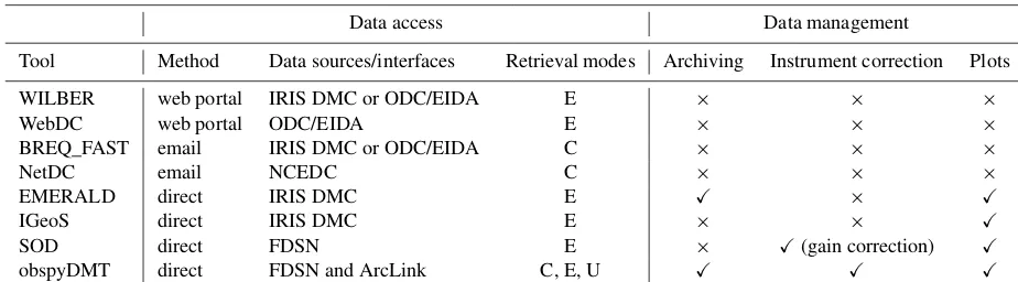
Various community software packages exist for achieving these tasks, but to our knowledge no other freely available package achieves them all. Table 1 compares the features of popular seismological community software to those of ob-spyDMT. We consider only tools that include functionality for data retrieval.

Table 1.Comparison of seismological data retrieval and management tools. Abbreviations: E – event-based; C – continuous time series; U – update mode. ObspyDMT is the only tool to provide access to both FDSN and ArcLink (in a single command), to retrieve both event-based and time-continuous waveform data, and to offer an “update” mode for waveforms, response files and/or metadata information. Few other tools provide for the management of data download and archiving, instrument correction, or diagnostics plots. EIDA: European Integrated Data Archive.

Data access Data management

Tool Method Data sources/interfaces Retrieval modes Archiving Instrument correction Plots

WILBER web portal IRIS DMC or ODC/EIDA E × × ×

WebDC web portal ODC/EIDA E × × ×

BREQ_FAST email IRIS DMC or ODC/EIDA C × × ×

NetDC email NCEDC C × × ×

EMERALD direct IRIS DMC E X × _X

IGeoS direct IRIS DMC E × × _X

SOD direct FDSN E × _X(gain correction) X

obspyDMT direct FDSN and ArcLink C, E, U X X X

are required, any given center needs to be contacted twice, using two different tools.

obspyDMT is the only tool among those in Table 1 that provides access to several data centers (in a single com-mand) and to both types of waveform data (in two sep-arate commands). The demand for continuous time se-ries, often in large quantities, has surged with the rapid rise in cross-correlation methods based on ambient noise (Shapiro and Campillo, 2004). ObspyDMT provides more convenient access than the email-based tools BREQ_FAST or NetDC.

obspyDMT is also the only tool to offer an “update” mode for waveforms, response files and/or metadata information: relaunching a previous request will identify and retrieve only data that could not be retrieved earlier. Like obspyDMT, the SOD, IGeoS and EMERALD tools are stand-alone software that runs on the user’s computer rather than a data center server. All four communicate with data centers via the rel-atively new web services interfaces defined by the FDSN. Queries are formulated as URL strings (uniform resource lo-cators) that point to physical data resources over the inter-net. We refer to this access method as “direct”. Compared to older access methods, it can save much human intervention time by freeing the user from the need to click through web pages (WILBER, WebDC) or manage emails (BREQ_FAST, NetDC). SOD, IGeoS and EMERALD retrieve event-based waveforms only, i.e., queries are based on earthquake occur-rences.

The stand-alone tools obspyDMT and EMERALD addi-tionally manage the data download and archiving to a local computer, thus relieving users of additional tedious and time-consuming steps. Both include certain plotting options (more extensively in obspyDMT).

obspyDMT also offers full instrument correction based on RESP or StationXML station metadata, combined with diag-nostic plots of transfer functions for individual filter stages. SOD is the only other tool to offer instrument correction, but

this includes gain correction only, and it offers no diagnostic plots.

obspyDMT is the only tool to provide an automated update functionality for a user’s existing, local data holdings.

3 Guided tour of use cases

The purpose of this section is to turn the reader into a pro-ficient user of obspyDMT in the short space of a few pages. We demonstrate the most common use cases for the query, selection, retrieval and management of seismograms, meta-data and synthetic waveform. We list obspyDMT’s full set of options in Table 2, which should be consulted as a cross-reference during the various stops of this guided tour.

We will

1. query event metadata from different earthquake catalogs 2. query station metadata from different data centers 3. request waveform data for a subset of events

(“event-based mode”), from several different data centers 4. demonstrate how to update a local data set (“update

mode”)

5. query and download continuous time series in arbitrary, user-provided time windows (“continuous mode”) 6. speeding up data retrieval by parallelization and bulk

requests

7. demonstrate obspyDMT’s plotting capabilities as we go 8. apply instrument corrections to waveform data

obspyDMT is a command-line tool that consists of a single command

obspyDMT

usually followed by option flags to modify the default be-havior. Table 2 lists all available flag options, with explana-tions.

3.1 Querying earthquake metadata

First, we request event information from one of several supported seismicity catalogs, without downloading any waveforms yet.

obspyDMT - -datapath neic_event_dir - -min_date 1990-01-01 - -max_date

2017-01-01 - -min_mag 5.0 - -event_catalog NEIC_USGS - -event_info - -plot_seismicity

This obspyDMT command with seven option flags queries the NEIC catalog (- -event_catalog NEIC_USGS) for all events exceeding a magni-tude of 5.0 (- -min_mag) that happened between 1990 and 2016 (- -min_date, - -max_date).

- -plot_seismicity triggers the generation of the global seismicity map plot of Fig. 2. - -event_info

switches off the retrieval of actual seismograms so that only metadata are downloaded to a local directory named

neic_event_dir/(argument of- -data_path). This directory is created if necessary, and it is populated with the following subdirectory and files:

neic_event_dir EVENTS-INFO

catalog.txt catalog.ml

catalog_table.txt event_list_pickle logger_command.txt

Geographical restrictions for event (or station) queries are supported in rectangular or circular areas. For example, to extract only earthquake metadata for Indonesia, specify

lonmin/lonmax/latmin/latmaxas

- -event_rect 80/135/-15/35

Appended to the earlier command, this generates the map inset of Fig. 2b. Note the rendering of colored beach balls (deepest seismicity in the foreground). The global map of Fig. 2 also plots beach balls rather than simple black dots, but they do not become apparent at this zoom level.

3.2 Query of station metadata

Let’s say we plan to investigate earthquakes exceeding a magnitude of 6.0 that occurred in this Indonesian rectangle at depths above 100 km. We want to know which seismometers in the Global Seismic Network (GSN) were operational to record them from 1 February to 1 December 2014. We issue the following query:

obspyDMT - -datapath event_based_dir - -min_date 2014-02-01 - -max_date 2014-12-01 - -min_mag 6.0 - -max_depth 100 - -event_rect 80/135/-15/35

- -event_catalog NEIC_USGS - -net _GSN - -cha BHZ - -meta_data

The NEIC event catalog returns 16 matching earthquakes, metadata for which are stored in 16 separate subdirecto-ries of a local directory calledevent_based_dir. Each of the 16 event subdirectories holds a subdirectory called

availability.txtto which metadata were written de-scribing the GSN seismometers that were operational during the event. (Refer to Appendix A and Fig. A1 for a graphic depicting the full directory structure created by obspyDMT.) Only station metadata are requested, as specified by the mode flag - -meta_data. We want StationXML files for (all) stations in the GSN network (- -net _GSN), but only for the broadband, high-gain, vertical components of these sta-tions, as specified by channel flag- -cha BHZ. A subset of stations could be specified by the- -staflag, which sup-ports wildcarding *, like many obspyDMT options. Since the option is absent here, it defaults to_{- -sta *}, i.e., all sta-tions in the_GSNnetwork. (See Table 2 for defaults for all options.) The underscore in- -net _GSNmarks this as a virtual network, whereas the two regular networks IU and II would be queried by- -net "IU,II".

3.3 Requesting and retrieving waveform data in

event-based mode

Next, we retrieve the actual BHZ seismograms from the GSN network that were recorded during the 16 Indonesian earthquakes identified in Sect. 3.2. In our earlier obspyDMT command, only a few option flags need to be changed:

obspyDMT - -datapath event_based_dir - -min_date 2014-02-01 - -max_date 2014-12-01 - -min_mag 6.0 - -max_depth 100 - -event_rect 80/135/-15/35

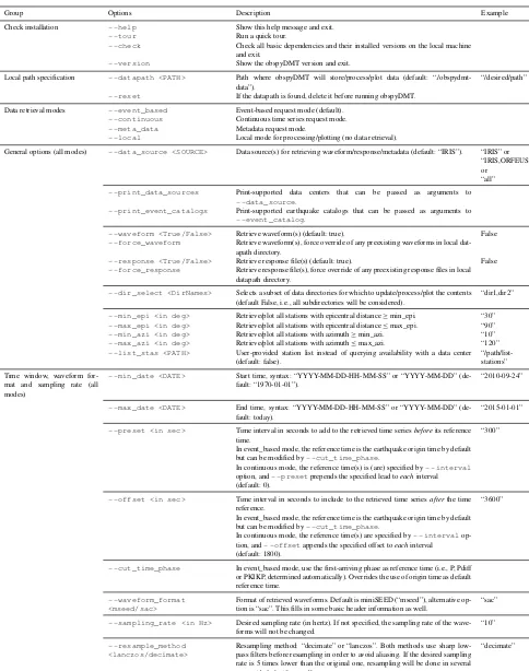
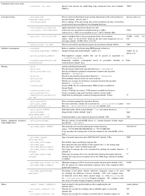
Table 2.Complete list of option flags to customize the default behavior of theobspyDMTcommand.

Group Options Description Example

Check installation - -help Show this help message and exit.

- -tour Run a quick tour.

- -check Check all basic dependencies and their installed versions on the local machine and exit.

- -version Show the obspyDMT version and exit.

Local path specification - -datapath <PATH> Path where obspyDMT will store/process/plot data (default: “./obspydmt-data”).

“/desired/path”

- -reset If the datapath is found, delete it before running obspyDMT.

Data retrieval modes - -event_based Event-based request mode (default).

- -continuous Continuous time series request mode.

- -meta_data Metadata request mode.

- -local Local mode for processing/plotting (no data retrieval).

General options (all modes) - -data_source <SOURCE> Data source(s) for retrieving waveform/response/metadata (default: “IRIS”). “IRIS” or “IRIS,ORFEUS” or

“all”

- -print_data_sources Print-supported data centers that can be passed as arguments to

- -data_source.

- -print_event_catalogs Print-supported earthquake catalogs that can be passed as arguments to

- -event_catalog.

- -waveform <True/False> Retrieve waveform(s) (default: true). False

- -force_waveform Retrieve waveform(s), force override of any preexisting waveforms in local dat-apath directory.

- -response <True/False> Retrieve response file(s) (default: true). False

- -force_response Retrieve response file(s), force override of any preexisting response files in local datapath directory.

- -dir_select <DirNames> Selects a subset of data directories for which to update/process/plot the contents (default False, i.e., all subdirectories will be considered).

“dir1,dir2”

- -min_epi <in deg> Retrieve/plot all stations with epicentral distance≥min_epi. “30”

- -max_epi <in deg> Retrieve/plot all stations with epicentral distance≤max_epi. “90”

- -min_azi <in deg> Retrieve/plot all stations with azimuth≥min_azi. “10”

- -max_azi <in deg> Retrieve/plot all stations with azimuth≤max_azi. “120”

- -list_stas <PATH> User-provided station list instead of querying availability with a data center (default: false).

“/path/list-stations”

Time window, waveform for-mat and sampling rate (all modes)

- -min_date <DATE> Start time, syntax: “YYYY-MM-DD-HH-MM-SS” or “YYYY-MM-DD” (de-fault: “1970-01-01”).

“2010-09-24”

- -max_date <DATE> End time, syntax: “YYYY-MM-DD-HH-MM-SS” or “YYYY-MM-DD” (de-fault: today).

“2015-01-01”

- -preset <in sec> Time interval in seconds to add to the retrieved time seriesbeforeits reference time.

In event_based mode, the reference time is the earthquake origin time by default but can be modified by- -cut_time_phase.

In continuous mode, the reference time(s) is (are) specified by- -interval

option, and- -presetprepends the specified lead toeachinterval (default: 0).

“300”

- -offset <in sec> Time interval in seconds to include to the retrieved time seriesafterthe time reference.

In event_based mode, the reference time is the earthquake origin time by default but can be modified by- -cut_time_phase.

In continuous mode, the reference time(s) are specified by- -interval op-tion, and- -offsetappends the specified offset toeachinterval

(default: 1800).

“3600”

- -cut_time_phase In event_based mode, use the first-arriving phase as reference time (i.e., P, Pdiff or PKIKP, determined automatically). Overrides the use of origin time as default reference time.

- -waveform_format <mseed/sac>

Format of retrieved waveforms. Default is miniSEED (“mseed”), alternative op-tion is “sac”. This fills in some basic header informaop-tion as well.

“sac”

- -sampling_rate <in Hz> Desired sampling rate (in hertz). If not specified, the sampling rate of the wave-forms will not be changed.

“10”

- -resample_method <lanczos/decimate>

Resampling method: “decimate” or “lanczos”. Both methods use sharp low-pass filters before resampling in order to avoid aliasing. If the desired sampling rate is 5 times lower than the original one, resampling will be done in several stages (default: “lanczos”).

Table 2.Complete list of option flags to customize the default behavior of theobspyDMTcommand.

Stations (all modes) - -net <NET> Network code (default: *). “TA” or

“TA,G” or “T*” or “*”

- -sta <STA> Station code (default: *). “RR01” or “RR01,RR02” or

“R*” or “*”

- -loc <LOC> Location code (default: *). “00” or “*”

- -cha <CHA> Channel code (default: *). “BHZ” or “BHZ,BHE” or “BH*” or “*”

- -identity <NET.STA.LOC.CHA> Identity code restriction, syntax: net.sta.loc.cha, e.g., IU.*.*.BHZ to search for All BHZ channels in IU network (default: *.*.*.*).

“IU.*.*.BH*”

- -station_rect

<lonmin/lonmax/latmin/latmax>

Include all stations within the defined rectangle,

syntax:<lonmin>/<lonmax>/<latmin>/<latmax>.

Cannot be combined with circular bounding box (- -station_circle) (default: -180.0/+180.0/-90.0/+90.0).

“20/30/-15/35”

- -station_circle <lon/lat/rmin/rmax>

Include all stations within the defined circle, syntax:<lon>/<lat>/<rmin>/<rmax>.

Cannot be combined with rectangular bounding box (- -station_rect) (default: 0/0/0/180).

“20/30/10/80”

Speedup options (all modes) - -req_parallel Enable parallel waveform/response request. Retrieve several wave-forms/metadata in parallel.

- -req_np <num_thread> Number of thread to be used in- -req_parallel(default: 4). “8”

- -bulk Send a bulk request to an FDSN data center. Returns multiple seismogram chan-nels in a single request.

Can be combined with- -req_parallel.

- -parallel_process Enable parallel local processing of the waveforms, useful on multicore hard-ware.

- -process_np <num_thread> Number of threads to be used in- -parallel_process(default: 4). “8”

Restricted data - -user <username> Username for restricted data requests, waveform/response modes (default: none).

“your_username”

- -pass <password> Password for restricted data requests, waveform/response modes (default: none).

“your_password”

Event-based mode - -event_catalog <CATALOG> Event catalog, currently supports LOCAL, NEIC_USGS, GCMT_COMBO, IRIS, NCEDC, USGS, INGV, ISC (default: LOCAL).

- -event_catalog LOCALsearches for an existing event catalog on the user’s local machine, in theEVENTS-INFOsubdirectory of- -datapath <PATH>. This is usually a previously retrieved catalog.

“IRIS”

- -event_info Retrieve event information (metadata) without downloading actual waveforms.

- -read_catalog <PATH> Read in an existing local event catalog and proceed. Currently supported cata-log metadata formats: “CSV”, “QUAKEML”, “NDK”, “ZMAP”.

Format of the plain text CSV (comma-separated values) is explained in the ob-spyDMT tutorial.

Refer to ObsPy documentation for details on QuakeML, NDK and ZMAP for-mats.

“/path/to/file.ml”

- -min_depth <in km> Minimum event depth (default: -10.0 (above the surface!)). “10”

- -max_depth <in km> Maximum event depth (default: +6000.0). “100”

- -min_mag <min_mag> Minimum magnitude (default: 3.0). “4.0”

- -max_mag <max_mag> Maximum magnitude (default: 10.0). “7.0”

- -mag_type <mag_type> Magnitude type. Common types include “Ml” (local/Richter magnitude), “Ms” (surface wave magnitude), “mb” (body wave magnitude), “Mw” (moment mag-nitude) (default: none, i.e., consider all magnitude types in a given catalog).

“Mw”

- -event_rect

<lonmin/lonmax/latmin/latmax>

Include all events within the defined rectangle,

syntax:<lonmin>/<lonmax>/<latmin>/<latmax>. Cannot be combined with circular bounding box (- -event_circle) (default: -180.0/+180.0/-90.0/+90.0).

“80/135/-15/35”

- -event_circle <lon/lat/rmin/rmax>

Search for all the events within the defined circle, syntax:<lon>/<lat>/<rmin>/<rmax>.

Cannot be combined with rectangular bounding box (- -event_rect) (default: 0/0/0/180).

“20/30/10/80”

- -isc_catalog

<COMPREHENSIVE/REVIEWED>

Search either the COMPREHENSIVE or the REVIEWED bulletin of the ISC. COMPREHENSIVE: all events collected by the ISC, including most recent events that are awaiting review.

REVIEWED: includes only events that have been relocated by ISC analysts. (default: COMPREHENSIVE).

Table 2.Complete list of option flags to customize the default behavior of theobspyDMTcommand. Continuous time series mode

- -interval <in sec> Specify time interval for subdividing long continuous time series (default: 86400 s).

“3600”

Local processing - -pre_process <name_process_unit>

Process retrieved data based on processing instructions in the selected process-ing unit (default: “process_unit”).

“process_unit_sac”

- -force_process Forces running of the processing unit on the local/retrieved data, overwriting any previously processed data in local datapath directory.

- -instrument_correction Apply instrument correction in the process unit.

- -corr_unit <DIS/VEL/ACC> Correct the raw waveforms for displacement inm(DIS), velocity inm/s(VEL) or acceleration inm/s2(ACC) (default: DIS).

“VEL”

- -pre_filt (f1,f2,f3,f4) Apply a bandpass filter to the seismograms before deconvolution,

syntax: “none” or “(f1,f2,f3,f4)” which are the four corner frequencies of a co-sine taper, default: “(0.008, 0.012, 3.0, 4.0)”.

“(0.008, 0.012, 3.0, 4.0)”

- -water_level <in dB> Water level in dB for instrument response deconvolution (default: 600.0). “300”

Synthetic seismograms - -syngine Retrieve synthetic waveforms using IRIS/syngine webservice.

- -syngine_bg_model <MODEL> Syngine background model (default: “iasp91_2s”). “iasp91_2s” or “prem_a_2s”

- -print_syngine_models Print-supported syngine models that can be passed as arguments to

- -syngine_bg_model.

- -syngine_geocentric_lat <True/False>

Requesting synthetic seismograms based on geocentric latitudes of events/stations (default: true).

False

Plotting - -plot Activates plotting functionality.

- -plot_sta Plot all stations found in the specified directory (- -datapath).

- -plot_availability Plot all availabilities (potential seismometers) found in the specified directory (- -datapath).

- -plot_ev Plot all events found in the specified directory (- -datapath).

- -plot_focal Plot beachballs instead of dots for event locations.

- -plot_ray Plot the ray coverage for all station–event pairs found in the specified directory (- -datapath).

- -create_kml Create a KML file for event/station/ray. KML format is readable by Google Earth.

- -create_event_vtk Create a VTK file for event(s). VTK format is readable by Paraview.

- -plot_seismicity Create a seismicity map and some basic statistics on the results.

- -depth_bins_seismicity <in km>

Depth bins for plotting the seismicity histogram (default: 10 km). “5”

- -plot_waveform Plot waveforms arranged by epicentral distance.

- -plot_dir_name <raw/processed/...>

Directory name that contains the waveforms for- -plot_waveformoption flag, e.g.,- -plot_waveform processed(default: raw).

“raw”

- -plot_save <PATH> Path where plots will be stored (default: “.”, i.e., the current directory). “.”

- -plot_format <png/jpeg/pdf/...>

Image format of plots (default: “png”). “png”

- -plot_lon0 <lon0> Central meridian (xaxis origin) for projection (default: 180). “160”

Explore instrument responses (stationXML files)

- -plot_stationxml Plot the contents of stationXML file(s), i.e., transfer function of filter stages, specified by- -datapath.

- -plotxml_date <DATE> Date and time to be used for plotting the transfer function, syntax: “YYYY-MM-DD-HH-MM-SS” or “YYYY-MM-DD”.

If not specified, the starting date of the last channel in the stationXML will be used.

“2010-01-01”

- -plotxml_output <DIS/VEL/ACC>

Type of transfer function to plot: DIS/VEL/ACC (default: VEL). “DIS”

- -plotxml_allstages Plot all filter stages specified in response file.

- -plotxml_paz Plot only poles and zeros (PAZs) of the response file, i.e., the analog stage.

- -plotxml_plotstage12 Plot only stages 1 and 2 of full response file.

- -plotxml_start_stage <stage>

First stage in response file to be considered for plotting the transfer function (default: 1).

“1”

- -plotxml_end_stage <stage>

Final stage in response file to be considered for plotting the transfer function, (default: last stage given in response file or the 100th stage, whichever number is smaller).

“3”

- -plotxml_min_freq <in Hz> Minimum frequency in Hz to be used in transfer function plots (default: 0.01). “0.001”

- -plotxml_map_compare Plot all stations for which instrument responses have been compared (PAZ against full response).

- -plotxml_percentage <percent>

Percentage of the phase transfer function’s frequency range to be used for checking the difference between methods. “100” will compare trans-fer functions across their entire spectral range, i.e., frommin_freq(set by- -plotxml_min_freq) to Nyquist frequency; “80” compares from min_freq to 0.8 times Nyquist frequency (default: 80).

“100”

Others - -email <email address> Send an email to the specified address after completing the job (default: false).

“email_address”

- -arc_avai_timeout <in sec>

Timeout (in seconds) for sending a data availability query via ArcLink (default: 40).

“60”

- -arc_wave_timeout <in sec>

Timeout (in seconds) for sending a waveform data or metadata request via ArcLink (default: 2).

Figure 2. obspyDMT - -datapath neic_event_dir - -min_date 1990-01-01 - -max_date 2017-01-01 - -min_mag 5.0 - -event_catalog NEIC_USGS - -event_info - -plot_seismicity

Global seismicity map of archived earthquakes in NEIC catalog of a magnitude of more than 5.0 that occurred between 1990 and 2016. One command queried the NEIC catalog, stored and organized the retrieved information and generated the seismicity map. (No actual waveform data were queried in this example.) The results of some basic statistics (magnitude and depth histograms) are also generated and plotted automatically(a). Note the rendering of colored beach balls in the map inset (deepest seismicity in the foreground). The global map also contains beach balls rather than just simple black dots, but they do not become apparent at this zoom level.

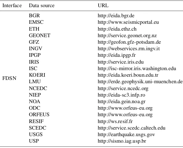
- -data_source specifies explicitly that the IRIS DMC should be contacted, although this would also be the default if the flag were omitted. If the user is unsure, it is best to specify- -data_source all, which prompts obspy-DMT to contact all 20 supported data centers listed in Table 3 and probably more in the future. (The list can be inspected by invokingobspyDMT - -print_data_sources.)

abso-Table 3. List of international data centers that can be currently accessed via FDSN and ArcLink interfaces of obspyDMT. This list is growing as more and more data centers can be accessed directly (as opposed to FTP or email-based methods). obspyDMT - -print_data_sourceslists all available data centers, and- -print_event_catalogslists all available event catalogs.

Interface Data source URL

FDSN

BGR http://eida.bgr.de

EMSC http://www.seismicportal.eu ETH http://eida.ethz.ch

GEONET http://service.geonet.org.nz GFZ http://geofon.gfz-potsdam.de INGV http://webservices.rm.ingv.it IPGP http://eida.ipgp.fr

IRIS http://service.iris.edu

ISC http://isc-mirror.iris.washington.edu KOERI http://eida.koeri.boun.edu.tr

LMU http://erde.geophysik.uni-muenchen.de NCEDC http://service.ncedc.org

NIEP http://eida-sc3.infp.ro NOA http://eida.gein.noa.gr ODC http://www.orfeus-eu.org ORFEUS http://www.orfeus-eu.org RESIF http://ws.resif.fr

SCEDC http://service.scedc.caltech.edu USGS http://earthquake.usgs.gov USP http://sismo.iag.usp.br ArcLink Many European data centers

lute start time. ObspyDMT knows that it is downloading in event-based mode because this is its default mode; adding the flag- -event_basedwould have made this explicit. (- -meta_datamode was introduced in Sect. 3.2; the al-ternative modes of- -continuousand- -localwill be demonstrated shortly.)

Issuing this single-line command is the only requirement on user time; everything else is done automatically. Specifi-cally, obspyDMT will do the following:

1. Request event information from the NEIC event catalog

- -event_catalog NEIC_USGS.

2. In the- -datapath event_based_dir, create a subdirectory EVENTS-INFO/containing a local cat-alog of metadata for the 16 matching events. Also in

- -datapath, create 16 event subdirectories, each containing a subdirectory tree (info/, resp/, raw/, pro-cessed/) as in Appendix A, Fig. A1.

3. Retrieve station metadata for all GSN stations for the 16 events in StationXML format from the IRIS data center and save these to subdirectoriesresp/.

4. Retrieve BHZ waveforms of 3900 s duration from all matching GSN stations in miniSEED format and save to subdirectoriesraw/.

5. Run default preprocessing operations on the waveforms, consisting of removing means and trends, tapering,

fil-tering, and deconvolving the instrument response (all customizable). The processed seismograms are save to subdirectoriesprocessed/.

6. Save additional log files on query success to subdirecto-riesinfo/.

Note how user time remains limited to issuing a sin-gle command no matter how many earthquakes, stations, or waveforms are being requested. Our tests required no human intervention even for very large requests that took weeks to download and encountered various time-outs or missing data issues at the data centers (cf. Sect. 4.2).

3.4 Update of existing waveform data sets

In the course of working with a waveform data set, it of-ten becomes necessary to update it. This could mean questing the same data again (because part of the earlier re-quest failed for some reason) or expanding the number of earthquakes, stations or seismograms. ObspyDMT aims to be smart about these various cases and not to retrieve du-plicates unless the users explicitly wants it to. We demon-strate typical use cases. They have in common that the local

- -datapath directorymust remain identical to that of any earlier request.

embargo period of a temporal network has ended), then it suffices to relaunch the exact same request (which was saved in log fileEVENTS-INFO/logger_command.txt):

obspyDMT - -datapath event_based_dir - -min_date 2014-02-01 - -max_date 2014-12-01 - -min_mag 6.0 - -max_depth 100 - -event_rect 80/135/-15/35

- -event_catalog NEIC_USGS - -net _GSN - -cha BHZ - -preset 300 - -offset 3600 - -instrument_correction - -data_source IRIS

obspyDMT compares the newly obtained event and station metadata to their local versions and downloads only holdings that differ.

If the user wants to update only certain events, then - -min_date, - -max_date, - -min_mag,

- -max_magand/or- -event_rectcan be adjusted (see Table 2 for other options). Similarly, if the new date–time window is not contained within the old one, then additional events might fit the criteria and their waveforms would be added in new event directories.

If all 16 preexisting event directories are to be updated, an alternative to the above command is to remove all event criteria because obspyDMT will then default to the local, preexisting event catalog in EVENTS-INFO/ for earthquake metadata.

obspyDMT - -datapath event_based_dir - -net _GSN - -cha BHZ - -preset 300 - -offset 3600 - -instrument_correction - -data_source IRIS

If the user decides they need seismograms for all BHE channels (in addition to BHZ), the update command would be

obspyDMT - -datapath event_based_dir - -net _GSN - -cha BHE - -preset 300 - -offset 3600 - -instrument_correction - -data_source IRIS

Augmenting the existing 16 events with seismograms from additional data centers is also an update operation because the waveform holdings of data centers often over-lap to some extent. Again obspyDMT will automatically compare metadata in order to avoid downloading duplicates. To update the data set with all vertical broadband chan-nels of the GFZ and ORFEUS data centers, we would request

obspyDMT - -datapath event_based_dir - -cha BHZ - -preset 300 - -offset 3600 - -instrument_correction - -data_source "GFZ,ORFEUS"

- -datapath event_based_dir is identical to what we defined in the previous command line that specifies the name of the top directory.

3.5 Retrieval of waveform data in time-continuous

mode (- -continuous)

In contrast to the examples thus far, some usage cases require waveforms that are not relative to or centered on specific earthquake occurrences. We refer to this usage mode as “time continuous” (- -continuous). For example, studies that cross-correlate ambient noise often require long time series from many stations, often divided into segments of shorter duration (i.e., 1 day). ObspyDMT makes the handling of continuous time series easy, even if the data sets are voluminous.

obspyDMT - -continuous - -datapath

yv_continuous_dir - -min_date 2012-12-15 - -max_date 2013-01-15 - -net YV

- -sta "RR0*,RR1*,RR2*" - -cha BHZ - -sampling_rate 10 - -data_source RESIF - -user your_username - -pass your_password

This command queries the French RESIF data center for time series from 15 December 2012 to 15 January 2013 recorded by the temporary ocean-bottom seismometer net-work of the RHUM-RUM (Réunion Hotspot and Upper Mantle – Réunions Unterer Mantel) experiment (network code YV) (Barruol and Sigloch, 2013; Stähler et al., 2016). The wildcard “*” is used to specify multiple station names. Since the data are embargoed until the end of 2017, a user-name and password needed to be passed to the data cen-ter (- -user, - -pass). Here we were interested in noise levels on the ocean floor during the passage of tropical storm Dumile and therefore requested waveforms for the storm pe-riod, highlighted by the yellow box in Fig. 3. The storm was clearly recorded by elevated noise levels, whose variable on-set times track the storm’s diachronous passage across the 1500 km×1500 km wide network (Davy et al., 2014).

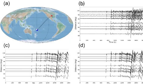
Figure 3. obspyDMT - -continuous - -datapath yv_continuous_dir - -min_date 2012-12-15 - -max_date 2013-01-15 - -net YV - -sta "RR0*,RR1*,RR2*" - -cha BHZ - -sampling_rate 10 - -data_source RESIF - -user your_username - -pass your_password

Retrieval of continuous time series of arbitrary length, here for 30 days in 2012/2013. Data are from the temporary ocean-bottom network RHUM-RUM (network YV, station names RR*) and are currently still password-protected at the RESIF data center (- -user, - -pass). The command specifies downsampling to 10 Hz immediately upon retrieval. The passage of the tropical storm Dumile is highlighted by the yellow box.

3.6 Speeding up data retrieval by parallelization

obspyDMT uses ObsPy clients to retrieve metadata and ac-tual waveforms from the data centers. Every request consists of three basic steps: (1) connect and send the data request to the data center; (2) download the data; (3) disconnect. By default, obspyDMT executes these steps for every metadata or waveform request separately, e.g., 3×1000 steps if 1000 waveforms are requested. For large requests, this can become a serious bottleneck. To increase the efficiency in such cases, a functionality for parallelized data retrieval can be enabled as follows:

- -req_parallel - -req_np 4

The first flag changes the data retrieval mode from se-rial (default) to parallelized, and the second flag specifies the number of parallel requests.

The parallelization in obspyDMT is implemented on two levels: data center and waveforms. As an example of the for-mer, if waveform data from both ORFEUS and IRIS are re-quested, obspyDMT sends parallel requests to these data cen-ters.

The other parallelization is at waveform level: if several waveforms are requested from one data center, they are re-trieved by- -req_npparallel processes. (A good choice for

npis the number of CPUs on the retrieving computer, i.e., 4 to 16 for many current laptops or desktops.) The number of requested waveforms or metadata files will be divided into

the number of specified processes. Each process then sends and retrieves its set of requests serially, but all processes or-ganize their data into the same- -datapathdirectory.

Further speeding up can be achieved by specifying a bulk request (- -bulkflag). Instead of requesting individ-ual items, this will send a list of items (time series or meta-data) to the data center, which reduces the number of (dis-)connections. We have, however, noticed occasional instabil-ities (for very large requests, fewer waveforms are retrieved than in serial mode); hence, serial is set as the conservative default.

3.7 Plotting tools

obspyDMT offers various plotting tools for visualizing data sets. Figure 2 demonstrates the plotting of seismic sources (beach balls) on a map, via the- -plot_seismicity op-tion.

Figure 4 demonstrates a map plot of ray paths between sources and receivers for the Indonesian example data set of Sect. 3.1 to 3.4 in Google Earth:

obspyDMT - -datapath event_based_dir - -local - -plot_ev - -plot_focal - -plot_sta - -plot_ray - -create_kml

mech-anisms (- -plot_focal), stations (- -plot_sta), and ray paths (- -plot_ray). One file in KML format is cre-ated (- -create_kml), which can be displayed by Google Earth. If- -create_kmlis omitted, obspyDMT plots the contents of the data set in maps similar to Figs. 2 or 5 (refer to Sect. 3.9). The flag- -localexplicitly tells obspyDMT to operate on preexisting content in the local data path direc-tory, rather than making new contact with a data center.

3.8 Processing and instrument correction

obspyDMT can process the waveforms directly after retriev-ing the data, or it can process an existretriev-ing data set in a separate step (local mode). By default, obspyDMT follows process-ing instructions described in the process_unit.py file located in the /path/to/my/obspyDMT/obspyDMT

directory. This scripting file can be freely edited by the user and may include calls to external waveform pro-cessing programs such as ObsPy or SAC. This vastly expands the possibilities for waveform processing and lets users easily adapt and integrate functionality from earlier, non-obspyDMT workflows. Instructions in this file are written at the waveform level, and obspyDMT applies them to all waveforms in the entire data set (in serial or in parallel mode). The default file included in the current distribution, /path/to/my/obspyDMT/obspyDMT/ process_unit.py, can perform routine processing steps such as resampling, data format conversion and instrument correction. These steps can be accessed via dedicated option flags, each of which results in the execution of only the appropriate part of processing scriptprocess_unit.py

(see - -pre_processoption flag). Hence, a user requir-ing only these routine operations need not create or modify a processing script file. The operations include

1. resampling time series, for example, downsampling for ease of storage and handling (refer to Sect. 3.5 and

- -sampling_rateoption flag)

2. converting the format of retrieved wave-forms to SAC and filling in some head-ers by the simple inclusion of the

- -waveform_format sacoption flag

3. instrument correction which includes removing means and trends, tapering, prefiltering (customizable by

- -pre_filt option flag) and deconvolving the in-strument response to displacement, velocity or acceler-ation (all customizable).

As an example, to correct the waveforms for instrument response directly after retrieving the data (similar to the ex-ample of Sect. 3.3)

obspyDMT - -datapath event_based_dir - -min_date 2014-02-01 - -max_date 2014-12-01 - -min_mag 6.0 - -max_depth 100 - -event_rect 80/135/-15/35

- -event_catalog NEIC_USGS - -net _GSN - -cha BHZ - -preset 300 - -offset 3600 - -instrument_correction - -data_source IRIS - -corr_unit VEL

- -corr_unit VEL specifies the physical unit of the processing output, in this case ground velocity in meters per second. The same data set can be corrected for displacement in a separate step (not directly after retrieving the data):

obspyDMT - -datapath event_based_dir - -local - -force_process

- -instrument_correction - -corr_unit DIS

Since obspyDMT stores processed waveforms in the

processeddirectory (Fig. A1), good practice is to rename allprocesseddirectories before launching the above com-mand line; otherwise, previously processed waveforms will be overwritten (- -force_process).

The user can also modify the process_unit.py

or write a new script with new processing instruc-tions. Currently, these files need to be located in the

/path/to/my/obspyDMT/obspyDMT directory and can be accessed via- -pre_process my_proc_unit

option flag, replacingmy_proc_unitwith the name of the Python script. The instructions are written at the waveform level, and obspyDMT automatically applies them to all archived waveforms. The main advantage of this design choice is its flexibility. The user can customize the processing instructions using available tools in ObsPy; moreover, other processing tools can be used or combined to write these in-structions. As an example, the following command line calls a processing instruction process_unit_sac.py; this file is located in/path/to/my/obspyDMT/obspyDMT:

obspyDMT - -datapath event_based_dir - -local - -force_process - -pre_process process_unit_sac

Here, SAC (instead of ObsPy) is used to remove the mean, apply a Hanning window, compute the FFT (fast Fourier transform), plot the amplitude spectrum of each waveform on a log–log plot and save the images as PDF files in the

processeddirectory.

3.9 Requesting synthetic seismograms

Figure 4. obspyDMT - -datapath event_based_dir - -local - -plot_ev - -plot_focal - -plot_sta - -plot_ray - -create_kml

Plot of the contents of the- -datapath event_based_dirthat contains the Indonesian example data set generated in Sects. 3.1 to 3.4.- -localspecifies that the existing, local waveform holdings should be plotted, rather than contacting the data centers anew. Sixteen earthquake locations are plotted as beach balls; stations featuring BHZ channels are indicated by yellow markers. Waveforms were retrieved from three data centers (IRIS, ORFEUS, GFZ).

waveforms from a new IRIS web service: Syngine (Krischer et al., 2017) and (2) providing required metadata for calcu-lating synthetic waveforms using external tools.

Syngine delivers fully numerical seismic waveforms computed on common spherically symmetric Earth models (PREM – Preliminary Reference Earth Model; ak135-f; IASP91). The following example command retrieves not only observed waveforms but also their synthetic counter-parts, computed on a PREM (Dziewonski and Anderson, 1981) anisotropic background model:

obspyDMT - -datapath data_fiji_island - -min_mag 6.8 - -min_date 2014-07-21 - -max_date 2014-07-22 - -event_catalog NEIC_USGS - -data_source IRIS - -min_azi 50 - -max_azi 55 - -min_epi 94 - -max_epi 100 - -cha BHZ - -instrument_correction - -syngine - -syngine_bg_model prem_a_2s

The two option flags that triggered the synthetic waveform retrieval are- -syngineand- -syngine_bg_model

prem_a_2s. The option flags - -min_azi,

- -max_azi, - -min_epi and - -max_epi spec-ify minimum azimuth, maximum azimuth, minimum distance and maximum distance for station search, re-spectively. The synthetic waveforms are stored in the

syngine_prem_a_2s directory, the contents of which can be plotted by obspyDMT plotting tools (refer to Fig. 5).

Changing the argument of- -syngine_bg_modelto

iasp91_2s, synthetic seismograms based on the IASP91 (Kennett and Engdahl, 1991) background model can be retrieved (Fig. 5):

obspyDMT - -datapath data_fiji_island - -min_mag 6.8 - -min_date 2014-07-21 - -max_date 2014-07-22 - -event_catalog NEIC_USGS - -data_source IRIS - -min_azi 50 - -max_azi 55 - -min_epi 94 - -max_epi 100 - -cha BHZ - -instrument_correction - -syngine - -syngine_bg_model iasp91_2s

Figure 5. Observed versus modeled broadband seismograms for an earthquake of a magnitude of 6.9Mw in the Fiji Islands region (21 July 2014, 14:54:41, at 19.802◦S, 178.4◦W; 615 km depth).(a)Source and receiver distribution plotted byobspyDMT - -datapath data_fiji_island - -local - -plot_ev - -plot_focal - -plot_sta - -plot_ray. Note the distribution of stations with respect to the event. The options flags- -min_azi, - -max_azi, - -min_epiand - -max_epispecified minimum azimuth, maximum azimuth, minimum distance and maximum distance for station search, respectively.(b)Observed broadband waveforms plot-ted byobspyDMT - -datapath data_fiji_island - -local - -plot_waveform - -plot_dir processed.(c) Syn-thetic seismograms retrieved from the Syngine web service for the PREM anisotropic background model. The stored waveforms are plotted

by obspyDMT - -datapath data_fiji_island - -local - -plot_waveform - -plot_dir syngine_prem_a_2s.

Panel (d) is similar to (c) except for the IASP91 background model. Plotted byobspyDMT - -datapath data_fiji_island

- -local - -plot_waveform - -plot_dir syngine_iasp91_2s.

obspyDMT - -print_syngine_models

Alternatively, metadata information and log files generated and organized by obspyDMT can be used to link an archived data set to other software for the generation of synthetic seis-mograms. A practical example of this is multiple-frequency tomography. In this method, frequency-dependent observ-ables (phase shifts or amplitudes) are measured by cross-correlating the recorded waveforms with the corresponding synthetic seismograms in multiple frequency bands (Sigloch, 2008; Zaroli et al., 2015; Hosseini and Sigloch, 2015). Syn-thetic seismograms need to be computed for exactly the same sources and receivers in the data set. This includes source characteristics (epicenter, depth, moment tensor and source time function) and receiver specifications (latitude, longi-tude, elevation and burial).

obspyDMT stores station information in one ASCII file per event and in the SAC headers (if this waveform format is selected). It automatically updates metadata information and

log files of a local data archive if stations are added/removed. Event information is written in QuakeML and ASCII for-mats. Although basic source and receiver information can be retrieved from most data centers, moment tensor solutions are available only in certain seismicity catalogs, among them the NEIC and GCMT catalogs, which are both supported by obspyDMT (refer to moment tensor retrieval as demonstrated by Fig. 2).

4 Discussion

Here we discuss implementation and performance issues, specifically obspyDMT’s communication with data centers, its robustness in the case of large and heterogeneous requests, and the usefulness of the instrument correction diagnostics. All three features set obspyDMT apart from existing tools.

4.1 Communication with data centers

obspyDMT can retrieve data from a multitude of interna-tional data centers (Table 3; a list that is growing). The user is shielded from having to know communication specifics for each data center. Under the hood, the software implements ObsPy clients for two different kinds of data exchange pro-tocols: FDSN web services and ArcLink.

In 2013, the FDSN defined common web service in-terfaces (http://www.fdsn.org/webservices/), allowing data request tools to work with any of the growing num-ber of FDSN data centers that implement these interfaces (http://www.fdsn.org/webservices/datacenters/). These cen-ters currently include the IRIS DMC, BGR, EMSC, ETH, GEONET, GFZ, INGV, IPGP, ISC, KOERI, LMU, NCEDC, NIEP, NOA, ODC, ORFEUS, RESIF, SCEDC, USGS and USP. Three service interfaces are specified by the FDSN and supported by ObsPy: fdsnws-station for accessing sta-tion metadata in Stasta-tionXML format, fdsnws-dataselect for accessing time series in miniSEED format, and fdsnws-event for accessing earthquake parameters in QuakeML format. ObspyDMT offers conversion to other formats, e.g., SAC for waveforms- -waveform_format sac. Requests are sent via the HTTP internet protocol for individual requests and via HTTP-POST for lists of requests, so that data can be requested from any web browser by generating URLs.

ArcLink is an older data request protocol that arose in Europe in order to virtually consolidate distributed seis-mological data holdings across various European countries. It is a distributed request protocol developed by the Ger-man WebDC initiative of GEOFON and BGR (Bunde-sanstalt für Geowissenschaften und Rohstoffe) as a contin-uation of the NetDC concept originally developed by the IRIS DMC. ArcLink communicates via TCP/IP rather than via supervision-intensive email or FTP requests required by other access mechanisms at the time. It accesses waveform data in miniSEED or SEED format and associated meta-information as dataless SEED files. At the time we developed ObsPyLoad, a pre-cursor of obspyDMT (Scheingraber et al., 2013), only a few data centers were implementing FDSN web services. Hence, ArcLink clients greatly expanded the reach of ObsPyLoad, to include most European data cen-ters. ObsPyLoad contacts the ORFEUS DMC via ArcLink, which in turn “forwards” ArcLink requests to other data cen-ters across Europe. This ArcLink functionality is retained in obspyDMT, but if a data center implements both interfaces, then obspyDMT accesses it via web services (default), which

Figure 6. obspyDMT - -plot_stationxml - -plotxml_paz - -plotxml_min_freq 0.0001 - -datapath /path/to/STXML.IC.XAN.00.BHZ

Transfer function spectra (amplitude and phase) of a Streck-eisen STS-1VBB w/E300 station (IC.XAN) in China. Blue lines show the transfer function components computed for all filter stages in a StationXML file; red lines are for the analog part. The two functions match very well in all frequencies except for the amplitude spectra close to the Nyquist frequency (dashed line).

now includes the European data centers. It seems likely that web services will completely supersede ArcLink.

4.2 Robustness of data retrieval

In our research we have used obspyDMT extensively, in order to retrieve several voluminous, event-based data sets for global-scale tomography, from different combinations of data centers. We have also requested large volumes of time-continuous data (“ambient noise”) for cross-correlation stud-ies. In all cases, we observed obspyDMT to work stably, i.e., requiring no user intervention despite the fact that many in-dividual waveform requests encounter errors from the data centers, for various reasons. ObspyDMT caught all excep-tions and continued undeterred.

Figure 7. obspyDMT - -plot_stationxml - -plotxml_paz - -plotxml_min_freq 0.0001 - -datapath /path/to/STXML.GT.LBTB.00.BHZ

Transfer function spectra (amplitude and phase) of a Geotech KS-54000 borehole seismometer (GT.LBTB) in Botswana. Blue lines show transfer function components computed for all filter stages in the StationXML file; red lines are for the analog part. A large discrepancy exists between the phase spectra of the two transfer functions. The deviation emerges at frequencies around 10−2Hz and increases up to the Nyquist frequency. Fig. 8 shows that this difference is caused by one of the digital stages in the instrument response.

communicate with all data centers, including some that im-plemented web services very recently.

obspyDMT - -datapath 2014_2015_dataset - -min_date 2014-01-01 - -max_date

2016-01-01 - -min_mag 6.0 - -event_catalog NEIC_USGS - -cha BHZ - -data_source

all - -preset 300 - -offset 3600

- -req_parallel - -req_np 8 - -pre_process False

The retrieval took 2 days and 10 h on a standard desktop with 4 CPUs. The retrieved data set was 145 GB in size, con-taining 293 events and 685 388 waveforms. No user interven-tion was required at any stage.

This finding is consistent with the performance of obspy-DMT’s predecessor ObsPyLoad (Scheingraber et al., 2013). With an event-based request similar to the one above to all data centers available at the time (in 2012 this was IRIS and the European centers via ORFEUS/ArcLink), we retrieved

162 GB of waveform data, consisting of 690 503 miniSEED files for three components (BHZ, BHE and BHN) for 154 events. The retrieval took 45 days because the job slowed down considerably after the first 73 GB (but continued at the old speed after relaunching, i.e., requesting the remaining 89 GB through update mode). The fraction of successfully re-trieved waveforms varied strongly between data centers and ranged from 99.8 to 34.8 % (availabilities were verified by spot checks in manual retrieval attempts). The exact reasons for the slowdown remained unclear, but aside from the deci-sion to relaunch, no user intervention was required at either download stage.

For the current test in 2017, no such slowdown was observed, and the retrieval of a comparable data volume (145 GB) took only a 1 / 20 of the time (2.5 days), despite being routed to many more data centers. We conclude that obspyDMT works robustly with all supported data centers, even for large and heterogeneous data and metadata requests.

4.3 Instrument correction

If station metadata could be routinely trusted, correcting for instrument responses would amount to a simple series of de-convolutions of a number of impulse responses (analog and digital filter stages from raw waveforms). Unfortunately, it is not uncommon for filter information in station metadata files to be erroneous. Some of the resulting artifacts in the dis-placement or velocity seismograms are large enough to po-tentially cause serious geoscientific misinterpretation, such as pronounced travel time delays under an isolated island sta-tion where in reality there are none.

Problems with the contents of StationXML or SEED/RESP files may or may not be straightforward to identify, as discussed below. A full visual representation of filter impulse responses can greatly facilitate trouble shooting. ObspyDMT implements several plotting options for this purpose, as demonstrated in Sect. 3.8 and Figs. 6–8.

An instrument response typically consists of a first, ana-log stage (a.k.a. “poles and zeros”, or PAZ stage), which de-scribes the transfer function of the sensor, and several digital stages, which describe the A/D conversion, antialiasing and downsampling inside the data logger. The PAZ stage is rarely problematic, whereas specifications of the digital stages are error-prone. Our discussion of neuralgic points and their pos-sible diagnosis follows the PhD thesis of Groos (2010).

Coefficients of asymmetric FIR filters are sometimes given in reverse order from that expected by the SEED convention, which can cause erroneous time delays of up to 1 s in the “corrected” waveforms. This issue may not be easy to detect as it requires knowledge of the correct order of filter coef-ficients, e.g., by comparing it to a trusted StationXML file describing the same data logger in a different location.

Figure 8. obspyDMT - -datapath /path/to/STXML.GT.LBTB.00.BHZ - -plot_stationxml - -plotxml_min_freq 0.0001 - -plotxml_allstages

Transfer function spectra (amplitude and phase) of each stage in the StationXML file of a Geotech KS-54000 borehole seismometer (GT.LBTB) in Botswana. In the phase response, two stages (1 and 5) have non-zero values. Both stages contribute to the phase spectrum of the complete instrument response (“full-resp”) of Fig. 7. However, the effects of Stage 5 on amplitude and phase spectra are not considered in PAZ (analog).

a potential problem. The very different phase responses of PAZ-only versus full response indicate that the digital stages introduce a significant delay (and possibly distortion) of the corrected time series. The user can then question whether this behavior is expected from the data logger. ObspyDMT automatically creates diagnostic reports for stations where PAZ and full response differ significantly. Figure 8 further zooms in on the issue, by indicating that among the digital stages, only Stage 5 has a non-zero phases response, identi-fying it as the questionable one. If the user decides that the digital stage specifications are suspect, they can choose to apply PAZ-only correction rather than full response – this should give a decent result, except for frequencies very close to Nyquist. Alternatively, if the user is working with low-frequency data only (below 0.01 Hz), they can conclude that no problem would ever arise because even Stage 5 is almost 0 in that spectral range.

Another recurring problem concerns delay time values specified for the FIR filter stages. According to the SEED manual, corrected filter delay times have to be positive; and yet, negative or 0 values are sometimes encountered in re-trieved metadata files which can result in erroneous time shifts of 1 to 2 s in corrected waveforms. This problem is eas-ily spotted, but 7 years after the report by (Groos, 2010), we still encounter such response files delivered by data centers.

obspyDMT also checks for inconsistencies in the “esti-mated delay” and the “correction applied” of the digital filter stages. In modern data loggers, these two values are usually similar because delay times are removed from the waveforms internally. However, discrepancies have been observed, such as negative or 0 values for the corrected delay time. In the ex-ample of Fig. 7, the estimated delay is reported as 0.63 s, and the applied correction is 0.0 s. ObspyDMT collects this in-formation and automatically generates one diagnostic report for the results of all consistency checks.

5 Conclusions

files into standardized directory trees. The user is provided with powerful diagnostic and plotting tools to check the re-trieved data and metadata. For large seismological data sets, data retrieval and processing can be parallelized on multi-core architectures by the simple inclusion of an option flag. Using obspyDMT’s diagnostic plots of analog and digital fil-ter stages, we checked the spectra (amplitude and phase) of instrument response files. Synthetic seismograms matching an example data set were retrieved from IRIS Syngine.

In all these use cases, issuing a single-line command is the only requirement for the user, everything else is done auto-matically.

Refer to Appendix C for instructions on how to download and install obspyDMT.

Appendix A: Directory structure

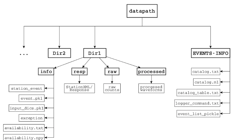
ObspyDMT organizes retrieved seismograms and metadata in a standardized directory structure, as shown in Fig. A1.

Figure A1.For each request, obspyDMT creates the depicted directory tree inside the user-specified directorydatapath/and arranges the retrieved data either in event subdirectories (for event-based requests) or in chronologically named subdirectories (for continuous requests). It also creates a subdirectoryEVENTS-INFO/in which a catalog of all requested events or time spans is stored. Earthquake metadata (date and time, latitude, longitude, depth, magnitude, moment tensor, source time function) are stored in CSV and QuakeML formats (files

Appendix B: Instrument correction

Seismograms recorded by digital broadband seismometers are stored as digitized voltage signals called “raw counts”. The relation between this signal and ground motion (e.g., displacement) depends on the response functions of the seis-mometer and data logger components (sensor, amplifiers, A/D converters, digital filters). Each component is referred to as a “stage” characterized by a transfer function, and the entire system can be described by the cumulative transfer function, i.e., a product in the frequency domain of the in-dividual stage transfer functions. The instrument sensor, i.e., the analog measurement apparatus before A/D conversion, is referred to as the analog stage or the poles-and-zeros stage. Following the nomenclature of the SEED Manual (Ahern et al., 2012), its frequency responseGcan be written as

G(j ω)=SdA0 QN

n=1(j ω−rn) QM

m=1(j ω−pm)

. (B1)

r andpstand for zeros and poles of a system.N andMare the number of zeros and poles, respectively.Sd is the stage gain.A0is the normalization factor, which scales the ampli-tude of the poles-and-zeros polynomial to unity at a reference frequency (usually 1 Hz):

A0 QN

n=1(j ωref−rn) QM

m=1(j ωref−pm)

=1. (B2)

Grelates the ground motionV (input signal) to recorded raw countsRby (Scherbaum, 1996):

R(j ω)=G(j ω)×V (j ω), (B3)

in which, R(j ω) andV (j ω) are the Fourier transforms of raw counts and ground motion, respectively. Instrument re-sponse correction can be carried out by transforming the raw seismogramR(t )to the spectral domain, dividingR(j ω)by G(j ω) (deconvolution in time) and transforming the result back into the time domain, in order to obtain V (t ) in the physical units of displacement, velocity or acceleration.

Instrument responses are provided by data centers in dif-ferent formats. An older format called SEED describes trans-fer functions of all analog and digital stages in a seismome-ter and is hence sufficient to calculate the frequency response function of a seismic channel (G(j ω)in Eq. B3). In practice, this format is usually converted to human readable ASCII files called SEED RESP that can be read by other instru-ment correction software such as evalresp. Recently, FDSN defined a new format FDSN StationXML which contains the most important and commonly used structures of SEED metadata in XML representation (FDSN, 2015). Compared to SEED, StationXML simplifies and adds clarification to station metadata. All data centers that support FDSN web services deliver instrument responses in this format. Obspy-DMT can read and interpret both StationXML and SEED.

Appendix C: Installation and system requirements

C1 ObsPy

ObsPy (Beyreuther et al., 2010; Megies et al., 2011; Krischer et al., 2015) is currently running and tested on Linux (32 and 64 bit), Windows (32 and 64 bit) and Mac OS X. Please refer to the ObsPy web page for complete notes regarding ObsPy installation on different platforms.

In addition to Python and ObsPy tools, obspyDMT builds onNumPy, an extension for performing numerical calcula-tions on large arrays and matrices (van der Walt et al., 2011);

matplotlib, a popular plotting package (Hunter, 2007);

matplotlib basemap toolkit (Whitaker, 2015) to project the data on a map; andSciPy(Jones et al., 2001), a library for advanced math, signal processing or statistics. Most of these libraries are prerequisites for installing ObsPy and are used in obspyDMT.

C2 obspyDMT

Once working Python and ObsPy environments are avail-able, obspyDMT can be installed in different ways:

1. Install obspyDMT package locally (using PyPi). This

tends to be the most user-friendly option:

pip install obspyDMT

2. Install obspyDMT from the source code.The latest

version of obspyDMT is available on GitHub. After in-stallinggit:

git clone https://github.com/kasra-hosseini/ obspyDMT.git /path/to/my/obspyDMT

cd /path/to/my/obspyDMT

obspyDMT can be installed by:

pip install -e .

or

python setup.py install

obspyDMT can be used from a system shell without explicitly calling the Python interpreter. The following command checks the dependencies required for running the code properly:

obspyDMT contains various option flags for customizing the request. Each option has a reasonable default value, which the user can change to adjust obspyDMT option flags to a specific request. The following command displays all available options with their default values:

obspyDMT - -help

The options are grouped by topics. To display only a list of these topic headings, use

obspyDMT - -options

To see the full help text for only one topic (e.g., group 2), use