https://doi.org/10.5194/se-9-373-2018
© Author(s) 2018. This work is distributed under the Creative Commons Attribution 3.0 License.
Remote-sensing data processing with the multivariate regression
analysis method for iron mineral resource potential mapping:
a case study in the Sarvian area, central Iran
Edris Mansouri1, Faranak Feizi2, Alireza Jafari Rad1, and Mehran Arian1
1Department of Geology, Science and Research branch, Islamic Azad University, Tehran, Iran 2Department of Mining Engineering, South Tehran branch, Islamic Azad University, Tehran, Iran
Correspondence:Faranak Feizi ([email protected]) Received: 10 March 2017 – Discussion started: 13 March 2017
Revised: 31 January 2018 – Accepted: 5 February 2018 – Published: 28 March 2018
Abstract.This paper uses multivariate regression to create a mathematical model for iron skarn exploration in the Sarvian area, central Iran, using multivariate regression for mineral prospectivity mapping (MPM). The main target of this pa-per is to apply multivariate regression analysis (as an MPM method) to map iron outcrops in the northeastern part of the study area in order to discover new iron deposits in other parts of the study area. Two types of multivariate regression models using two linear equations were employed to dis-cover new mineral deposits. This method is one of the re-liable methods for processing satellite images. ASTER satel-lite images (14 bands) were used as unique independent vari-ables (UIVs), and iron outcrops were mapped as dependent variables for MPM. According to the results of the probabil-ity value (p value), coefficient of determination value (R2) and adjusted determination coefficient (R2adj), the second re-gression model (which consistent of multiple UIVs) fitted better than other models. The accuracy of the model was confirmed by iron outcrops map and geological observation. Based on field observation, iron mineralization occurs at the contact of limestone and intrusive rocks (skarn type).
1 Introduction
The remote-sensing layer is one of the significant data lay-ers which is applicable for different levels of mineral ex-ploration especially at reconnaissance levels. This data layer is processed based on the most common techniques for the identification of minerals. Mineral exploration is a complex
process (Gupta, 2003). The complexities of mineral explo-ration can be solved by using remote-sensing techniques in the early stages of mineral exploration for the reconnaissance of target areas with the goal of continuing exploratory opera-tions. One of the most recognizable uses with remote sensing is mineral exploration and the identification of various geo-logical structures, faults and lineaments, geogeo-logical units, al-terations, indicator, and tracer minerals (Melesse et al., 2007; Carranza, 2008; Abedi et al., 2013; Golshadi et al., 2016 and Feizi and Mansouri, 2012). The factors mentioned play im-portant roles for recognizing mineralization in the region of interest; so the identification of these factors saves time and cost as well as giving a more precise result (Xiong and Zuo, 2017).
There are various techniques in remote-sensing processes for recognizing minerals. The satellite images were pro-cessed with specific mathematical algorithms in all remote-sensing techniques with the goal of the generation of useful information. The information mentioned can be integrated with other information and layers for the evaluation and in-terpretation of exploratory results (Li et al., 2015, Abedi et al., 2012; Bonham-Carter and Agterberg, 1990; Carranza, 2009; Carranza and Sadeghi, 2010; Ford and Blenkinsop, 2008; Lindsay et al., 2014; Lisitsin et al., 2013; Pan and Har-ris, 2000; Porwal et al., 2010; Feizi and Mansouri, 2013a).
mathemat-ical basics and the fact that it is compatible with geologmathemat-ical data.
The identification of stream sediment anomalies has been used by multiple regression analyses (e.g. Carranza, 2010a, b). Likewise, multivariate regression has been effectively uti-lized by Granian et al. (2015) to display subsurface min-eralization from lithogeochemical information. Granian et al. (2015) used four types of multivariate regression mod-els to depict significant surface geochemical anomalies in-dicating subsurface gold mineralization and utilizing bore-hole data as dependent variables and surface lithogeochemi-cal data as independent variables.
Based on previous work such as Allbed et al. (2014), mod-elling and mapping of mineral potentials based on satellite image data and processing it based on remote-sensing and regression analysis is a promising approach as it facilitates timely detection with a low-cost procedure and allows deci-sion makers to decide what necessary action should be taken as the first step in the mineral prospectivity mapping (MPM) field.
There are multiple types of regression analyses. Among these types, multivariate regression analysis is selected and used in this paper. In multivariate regression analysis, the relationships between independent variables and dependent variables is predicted in order to analyse the effects of in-dependent variables on in-dependent variables. This method can be used in remote sensing by modelling the mineraliza-tion outcrop points for further exploramineraliza-tion and finding new prospective zones, directly. One of the advantages of this method is the directness and quickness of mineral identifi-cations without the need for other exploration layers.
The aim of this paper is the processing of satellite images by the mathematical method of regression analyses and us-ing its applications in remote-sensus-ing and geological units. In addition, recognizing new mineralization in the region of interest with modelling mines and known deposits is another purpose of this paper. This aim is reached by identifying geo-logical dependent variables and finding relationships among them for the exploration of new deposits with an acceptable accuracy in the study area.
The Sarvian iron ore deposit with 8 million tons reserve is a calcic iron skarn deposit. Due to intrusive rocks and carbon-ate rocks in many parts of the study area, new iron skarn min-eralization can be introduced. In this paper we used the re-gression method to identify new iron mineralization in other parts of the study area.
In order to perform this method, the existence of a de-pendent variable is the main condition for the use of ana-lytic regression. In this study, Advanced Spaceborne Ther-mal Emission and Reflection Radiometer (ASTER) satellite image pixels located in the northeastern part of the study area were considered to be dependent variables. Also, ASTER satellite image pixels of other parts of the study area were considered to be independent variables.
Two types of multivariate regression models were used to find new mineral deposits: the 14 bands of ASTER satel-lite images were set as unique independent variables (UIVs), while iron outcrop area (digitized as a 1 : 5000 geology map of the study area and field) data were set as dependent vari-ables.
2 Methodology 2.1 Study area
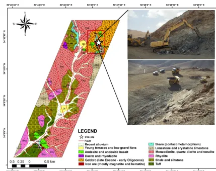
The Sarvian area is in the Or¯um¯ıyeh-Dokhtar magmatic arc in central Iran (Fig. 1a). This magmatic arc is the most impor-tant metallogenic area inside the district; it hosts large metal deposits such as lead, zinc, copper and iron. A set of crys-tallized limestone dolomite are the oldest geological units in the study area, dating to the Permian and Triassic. Sedimen-tation of limestone and marl in the Qom formation occurred concurrent with continental sedimentation at the Oligocene. Most tectonic activity in the study area was in the form of vertical movements ,which caused instability in the basin and changed the depth of the sea. Vertical movements at the be-ginning of the Miocene caused volcanic activity in the study area, which was impressive. Important magmatism occurred in the late of Miocene, which caused skarn mineralization where carbonate units of the Qom formation were in contact. The main fault of the study area is Bidehend. The Bidehend is a strike-slip fault with a length of 43 km. The Bidehend fault is 10 km away from the study area. The effect of this major fault on the study area is limited to the creation of parallel faults and fractures with the same direction as the Bidehend fault. There is no relationship between the skarn mineraliza-tion and faults in the Sarvian area because no mineralizamineraliza-tion has been reported in faults and fractures (Feizi et al., 2016, 2017).
The study area is dominated by Eocene intrusive rocks and carbonates of the Qom formation. Several types of metal and non-metal mineral ore deposits have, up to now, been re-ported in the study area. According to the 1 : 100 000 geolog-ical map of Kahak, the lithology of this area includes cream limestone with intercalations of marls (Qom formation), dark green, andesitic–basaltic lava, volcanic breccia, hyaloclas-tic limestone, green megaporphyrihyaloclas-tic andesihyaloclas-tic–basalhyaloclas-tic lava, rhyodacitic domes, tonalite–quartz-diorite, microquartz-diorite–microquartz-monzodiorite, granite–granodiorite, al-ternations between light green and grey tuff, tuffaceous sand-stone and shale with the intercalation of nummulitic sandy limestone and andesitic lava, andOrbitolina-bearing, thick-bedded to massive grey limestone (Aptian–Albian) (Feizi et al., 2016) (Fig. 1b).
Figure 1. (a)The location of the Sarvian area in the Or¯um¯ıyeh–Dokhtar magmatic belt, Iran.(b)Geological map of the Sarvian area (scale 1 : 25 000).
alteration are localized along the contact zone between intru-sive rocks and carbonate sequences (Zuo et al., 2014).
2.2 Multivariate regression
For uncovering relationships between independent and de-pendent variables, an appropriate statistical tool was intro-duced into geoscience by Granian et al. (2015) which is called regression analyses. If dependent variables are called
(Y )and independent variables are called (xi), the formula is
Y=f (xi). (1)
Based on regression analysis theory,Ycan be a linear or non-linear function. IfY is linear, the formula is
Y=a0+a1x1+a2x2+. . .+aixi+ε, i=1,2, . . ., n. (2)
For the formula mentioned, the constant factor isa0, the
Figure 2.Location of the Sarvian iron mine in the study area.
arensamples in a data set, for each sampletvariables were measured. Therefore, formula (2) can be written as
Yi= ˆa0+ ˆa1Xi1+ ˆa2Xi2+. . .+ ˆatXit+εi,
i=1,2, . . ., n. (3)
Formula (3) can be presented as a linear function matrix:
[Y]=[X] [A]+[ε] (4)
[Y]= Y1 Y2 .. . Yn
; [A]= ˆ a0 ˆ a1 .. . ˆ at ; [X]=
1 X11 X12 . . . X1t 1 X21 X22 . . . X2t
.. .
1 Xn1 Xn2 . . . Xnt ; [ε]= ε1 2 .. . n . (5)
For calculating the coefficient matrix [A] the least squares method is utilized:
[A]=hXi −1
[C]= [X]0[X]−1[X]0[Y]. (6)
The inverse of the variance–covariance sample matrix is P−1
, and the covariance matrix among independent vari-able and samples is [C]. So the regression coefficient model is computed by formula (6).
Based on Granian et al. (2015), the following criteria were utilized for the examination of the regression analysis:
1. The variance and the mean of the random error should be a constant value and zero, respectively.
2. The coefficient of determination value which is called (R2)should be tested (Granian et al., 2015).R2is pre-sented as
R2= Pn
i=1
ˆ Yi−Y
2
Pn
i=1 Yi−Y
2 =1−
Pn i=1
Yi− ˆYi
2
Pn
i=1 Yi−Y
3. Given the fact that adding independent variables to the model will increase theR2value, the adjusted determi-nation coefficient which is called (Radj2 )is presented as (Granian et al., 2015):
R2adjusted=1−n−1 n−t
1−R2. (8)
In Eq. (8),nis the number of data andtis the number of regression coefficients. If a set of explanatory variables are introduced into a regression one at a time, with the R2adjcomputed each time, the level at whichR2adjreaches a maximum, and decreases afterward, would be a well-fitted model.
4. In regression analyses, thepvalue of final coefficients for each specific model could be applied after choosing the best model. Accordingly, thepvalue of the regres-sion model in the analysis of variance (ANOVA) test should be acceptable (less than or equal to 0.05).
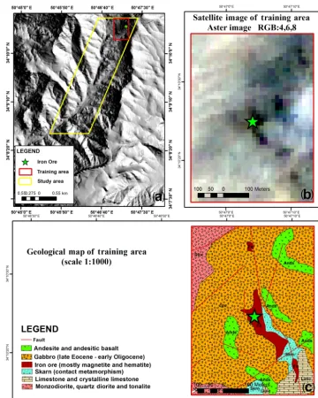
2.3 Data collection
There are several iron ore bodies and one iron mine in the northeastern Sarvian study area. The regional geological con-ditions of the area suggest that the Sarvian iron mine is a good model for exploring the surrounding area. In this pa-per, a geology map of the mine is used as a training area for satellite imagery. In the training area, this method can model the iron outcrops (a dependent variable) based on ASTER satellite image bands (independent variables) (Fig. 3). 2.3.1 Remote-sensing data (independent variables) The ASTER sensor was launched in December 1999 on board the Earth Observation System (EOS) US Terra satel-lite. ASTER provides high-resolution images of the land surface, water, ice, and clouds using three separate sensor subsystems covering 14 multi-spectral bands from visible to thermal infrared (Table 1). Resolutions are 15, 30 and 90 m in the visible and near infrared (VNIR), shortwave infrared (SWIR) and thermal infrared (TIR), respectively. For more information see Feizi and Mansouri (2013b) and Mansouri and Feizi (2016).
In this study after corrections, the pixel size of the SWIR and TIR bands based on the VNIR3 band (panchromatic band) was converted to 15 m. The layer stacking function was then used to build a new multiband file from georefer-enced images of various pixel sizes, extents and projections (Mansouri et al., 2015). The date of the images is 11 June 2002.
2.3.2 Mapping of iron outcrops (dependent variable) There are several iron veins and outcrops around the iron ore skarn mine in the northeastern part of the Sarvian area. Iron
outcrops in the training area were mapped using a geological map on a scale of 1 : 1000 of the iron ore deposit. The map was then field checked. The shape file layer of iron outcrops was converted to a raster file with a pixel size of 15 m.
3 Results
Multiple, factorial, polynomial and response surface regres-sions have been utilized in many fields including the geo-sciences (e.g. Granian et al., 2015). In this study, Model 1 (Y1)was generated as a multiple linear regression model and
Model 2 (Y2)was created fromY1plus many UIVs. The
for-mulas for the two models are presented in Table 2. Thus, two linear equations (Y1andY2)were used to discover new
min-eral deposits, using pixel values from ASTER satellite data as independent variables and a map of iron outcrops as de-pendent variables. Of the two models proposed in this paper, model 2 has 106 coefficients (14 for UIVs, 1 as constant, 91 for multiples of UIVs) and model 1 has 15 coefficients (14 for UIVs, 1 as constant, 0 for multiples and exponents of UIVs) (Table 2).
Regression analyses were performed to assess the models in Table 2, and the critical criteria mentioned above were ex-amined. TheR2,Radj2 andpvalues from the ANOVA test of two multivariate regression models are provided in Table 3.
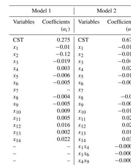
Table 4 presents the calculated coefficients of indepen-dent variables in regression models. Excluded indepenindepen-dent variables are not mentioned in Table 4. Excluded variables were those that had no effect on iron mineralization and the mapped distribution of iron outcrops.
We used several criteria to review the differences between the two models. Firstly, the variance and the mean of the ran-dom error were acceptable for both models. Secondly, based on Table 4, thepvalues of the ANOVA test of the two mod-els were equal to 0. For regression modmod-els, the acceptablep value should be less than or equal to 0.05. Thus, this criterion confirmed the validity of the models without specifying the most appropriate model.
The value ofR2is close to 1 for well-fitted models. TheR2 values of regression models are presented in Table 3. Model Y1has a lowerR2thanY2. Thus, theY2model is better than
theY1model.
Because adding independent variables to the model will increase theR2value, theR2adjvalue should be checked. The Radj2 values of regression models are presented in Table 3. As mentioned above, if a set of variables is introduced into a regression, with theR2adjcomputed each time, the level at whichRadj2 reaches a maximum, and decreases afterwards, would result in a well-fitted model. So, according to Table 3, Y2, as opposed to the other models, is the fitted model. Thus,
theY2 regression model is the most appropriate model for
mineral prospectivity mapping.
op-Figure 3. (a)Location of training area in the study area.(b)ASTER satellite image in the training area (RGB: 4, 6, 8).(c)Geological map (scale 1 : 1000) of training area.
Table 1.Wavelength ranges and spatial resolutions of ASTER bands (Abrams, 2000).
Module VNIR SWIR TIR
Spectral bandwidth (µm) Band 1 0.52–0.60 Band 4 1.650–1.700 Band 10 8.125–8.475
Band 2 0.63–0.69 Band 5 2.145–2.185 Band 11 8.475–8.825
Band 3 N 0.78–0.86 Band 6 2.185–2.225 Band 12 8.925–9.275 Band 3 B 0.78–0.86 (backward looking) Band 7 2.235–2.285 Band 13 10.25–10.95 Band 8 2.295–2.395 Band 14 10.95–11.65 Band 9 2.360–2.430
Table 2.Formula of regression models used for ASTER satellite image bands.
Types of Number of Formula regression coefficients
First-degree 15 Y1=a0+a1x1+a2x2+. . .+a14x14
First-degree 106 Y2=Y1+a15x1x2+a16x1x3+. . .+a27x1x14+a28x2x3+a29x2x4+. . .+a39x2x14+ a40x3x4+a41x3x5+. . .+a50x3x14+a51x4x5+. . .+a60x4x14+a61x5x6+. . .+ a69x5x14+a70x6x7+. . .+a77x6x14+a78x7x8+. . .+a84x7x14+a85x8x9+. . .+ a90x8x14+a91x9x10+. . .+a96x9x14+a97x10x11+. . .+a100x10x14+a101x11x12+ . . .+a103x11x14+a104x12x13+a105x12x14+a106x13x14
Table 3.TheR2,R2adjandpvalues of the ANOVA test of two mul-tivariate regression models.
Models R2 Radj2 pvalue (ANOVA)
Y1 0.738 0.715 0
Y2 0.847 0.829 0
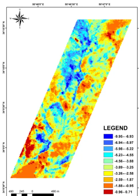
posed to the other models, would be the fitted model. For generating a mineral prospectivity map the model Y2 was
implemented in ArcGIS using the raster calculator tool. The normalized mineral prospectivity map of the study area is presented in Fig. 4.
4 Discussion
A large part of the study area is formed based on carbon-ate units of the Qom formation and intrusive rocks such as diorite, granodiorite and gabbro. These rock units increases the probability of skarn mineralization in the study area. The type of the Sarvian iron ore, which is used in this paper from its outcropping pixels as dependent variables, is also skarn. According to the observations in the field operations and the study of the geological map of the area, there is contact between the intrusive units (diorite, granodiorite) and host rocks (limestone and siltstone of the Qom formation). In the contact area of intrusive units and host rocks, the skarn geo-logical unit was seen as a narrow strip. The major economical mineralization of skarn iron ores in this region is magnetite.
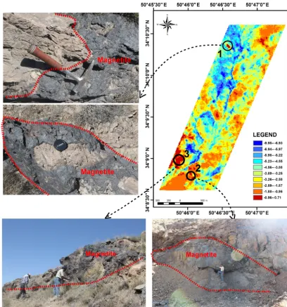
To assess the accuracy of the selected model, the created prospectivity map was checked against the iron outcrops map in the northeastern part of the study area (Fig. 5). The loca-tions of iron outcrops are in close agreement with predic-tions from the mineral prospectivity map. In addition, three target areas with very high potential were checked for iron outcrops, and the prospectivity map was confirmed by geo-logical observations (Fig. 6). Based on field observation, iron mineralization occurs at contacts between limestone and in-trusive rocks (skarn type). Iron mineralization consists
dom-Table 4.The calculated coefficients of regression models 1 and 2. CST indicates the constant.
Model 1 Model 2
Variables Coefficients Variables Coefficients
(ai) (ai)
CST 0.275 CST 0.677
x1 −0.01 x1 −0.014
x2 −0.12 x2 −0.019
x3 −0.019 x3 −0.045
x4 0.003 x4 0.022
x5 −0.006 x5 −0.017
x6 −0.005 x6 −0.001
x7 – x7 –
x8 −0.004 x8 −0.02
x9 −0.005 x9 −0.006
x10 0.009 x10 −0.014
x11 0.005 x11 0.024
x12 0.016 x12 0.024
x13 0.002 x13 0.018
x14 0.022 x14 0.036
– – x1x4 −0.0009
– – x1x6 −0.0002
– – x4x9 −0.0009
– – x7x8 0.00082
inantly of magnetite (Fig. 6). Therefore, the accuracy of the mineral prospectivity map is confirmed in the Sarvian area.
It is obvious that satellite images consist of various bands, and each pixel in different bands has a specific pixel value. Thus, some quantitative information is obtained which should be processed for reaching the goal of interest. In re-mote sensing, selecting the appropriate method and algo-rithm is significant for obtaining the best results.
Remote-sensing methods were mostly generated based on spectral or pixels. Based on this categorization, various statis-tical and spectral methods are available. One of the methods that can be used in remote sensing is analytical regression. This method is a statistical process for estimating the rela-tionships between variables.
sup-Figure 4.Mineral prospectivity map of the Sarvian area.
porting vector machine (SVM) technique is a supervised ap-proach which can be compared to multivariate regression analysis because both methods are supervised and based on regression functions.
The theory of SVM is based on classification and regres-sion. This method is one of the most recent approaches that has shown appropriate performance in recent years. The clas-sification in SVM is according to the linear data classifica-tion, and the user should select an appropriate line for classi-fication. This method is a linear training method which uses the empty spaces between data. The SVM uses kernel func-tions to separate and classify classes. The more kernels can locate the classes with maximum distance from each other, the greater the accuracy with which the classification will be done. This refers to the maximum distance between the sep-arator screen and the closest samples of each class (Forkuor et al., 2017; Cheng and Bao, 2014).
The most important advantages of SVM are that it has good application in various fields and produces an optimal re-sponse. The most important disadvantages of SVM are men-tioned below:
1. In SVM method an appropriate kernel should be se-lected. Determining the proper kernel is very important. Selecting an inappropriate kernel causes errors in calcu-lations and conclusions.
2. Accuracy sensitivity to SVM parameters.
3. SVM has limitations in speed and time because in this method an optimization issue needs to be solved. 4. This method may not provide good results for all data.
The similarity between SVM and the method used in this paper is that both are based on regression mathematics the-ory and functions, but there are also some differences be-tween them. The SVM classifies and separates the categories, but the analytic regression method uses existing relationships and correlations between the data for introducing the best possible model for predicting the result.
The most important advantages of the analytical regression method are mentioned below:
1. Almost all data can be used in this method.
2. The analytical regression method does not depend on a particular parameter, and it does not have any special restrictions like the SVM.
3. The analytical regression method does not have any lim-itations in speed and time.
4. Due to the fact that the model predicts the results ac-cording to the data as well as the relationships between the data, the results are closer to reality.
Forkuor et al. (2017) used four methods, i.e. multiple lin-ear regression (MLR), random forest regression (RFR), sup-port vector machine (SVM) and stochastic gradient boosting (SGB), to study soil properties in southwestern Burkina Faso. The results of all four methods are confirmed by Forkuor et al. (2017), who stated that other methods are preferable in comparison with methods based on regression according to the model performances statistics. This statement can obvi-ously not be accurate in iron ore exploration of the Sarvian area. The results of regression analyses in the Sarvian area showed that all of the areas predicted by the appropriate re-gression model are iron ore minerals.
Also Allbed et al. (2014) used regression analyses to iden-tify soil properties on satellite imagery and achieved good results; but the difference between this paper and other simi-lar papers is the use of regression analyses in mineral explo-ration as well as the geneexplo-ration of a mineral potential map.
To examine and compare the results of using multivariate analytic regression with other similar methods on mineral ex-ploration, Feizi and Mansouri (2013b) is used.
Figure 5.Mineral prospectivity map of the Sarvian area, which is confirmed by iron outcrops.
reasons. Firstly, the northern part of the study area in this pa-per is similar to some areas of the southern part of the study area in Feizi and Mansouri (2013b); secondly, like this paper, Feizi and Mansouri (2013b) is published with the aim of iron ore exploration. Feizi and Mansouri (2013b) used methods such as the Spectral Angle Mapper (SAM), principal compo-nent analysis (PCA), least-squares fit linear band prediction (LS-Fit), Minimum Noise Fraction Transform (MNF) and band ratio for iron ore exploration. According to the results obtained by these methods, the identified regions are iron ox-ide zones containing magnetite, hematite, goethite, limonite and jarosite minerals. In the Sarvian area, magnetite ore is more economical than other minerals and all active mines with more magnetite (in comparison with other minerals such as hematite, goethite, limonite and jarosite) are more eco-nomical. Therefore, the methods, such as SAM, PCA, LS-Fit, MNF and band ratio, used by Feizi and Mansouri (2013b) introduced iron oxide alterations and a variety of iron min-erals such as hematite, goethite, limonite, and jarosite with magnetite, which are not significant or economically valu-able. So, to identify the areas with the most magnetite, the field study should be performed with a high accuracy, which prevents wasting time and money; the results of multivari-ate regression in this paper recognized magnetite areas accu-rately. In this paper, the pixels for the magnetite veins of the Sarvian iron ore mine are considered to be base pixels, and, therefore, the results obtained from this method demonstrate exactly the magnetite anomalies in the study area. Iron oxide alterations and a variety of uneconomical iron minerals such
as hematite, goethite, limonite, and jarosite in the study area were not observed based on the results of multivariate re-gression. Thus, the multivariate regression method performs more accurately than other methods mentioned, which re-sults in saving time and money, specifically with regard to the field study. It should be noted that the use of analytical regression in remote sensing is most recent, and it needs fur-ther studies especially for different types of deposits in min-eral exploration.
The novelty of this paper is the use of regression analyses in mineral exploration as well as the generation of a mineral potential map. For mineral exploration, various geo-data lay-ers, such as geochemical, geophysical, remote sensing and geological geo-data layers, should be integrated into GIS, but the most important achievement of this method is that it can be used as a direct method for mineral exploration with the least requirement of other exploration layers. The direct de-tection of minerals such as copper, lead, zinc and some eco-nomically valuable minerals is difficult using remote sens-ing, but due to the accuracy of this method, these elements can be explored more easily than before. Selecting pixels as dependent variables has a direct effect on the results and is very important in regression analyses; therefore, the higher the resolution of the images, the more accurate the results will be.
5 Conclusion
Figure 6.Mineral prospectivity map of the Sarvian area, which was confirmed by a field sample of the three target areas.
1. Regression analysis is an appropriate and direct method for mineral prospectivity mapping (MPM) with satellite image data. In this paper, the output of processed satel-lite images using regression analysis indicates the iron potential zones accurately.
2. The application of multivariate regression analysis (as an MPM method) was confirmed in the Sarvian area. This paper used multivariate regression to create a math-ematical model (with reasonable accuracy) for iron min-eral exploration in the region of interest.
3. Two types of multivariate regression models, in the form of two linear equations, were employed to discover new mineral deposits. According to the results of the
pvalue,R2andR2adj, the second-regression model pro-vided the best appropriate observations.
4. The accuracy of the model was confirmed by iron out-crop mapping and geological observations. Based on field observation, iron mineralization occurs as contact between limestone and intrusive rocks (skarn type).
6. The regression analysis method is a subset of supervised classification due to the procedure mentioned. In this method, target spectrums of the training area are used for modelling and MPM.
Data availability. ASTER satellite image data used in this pa-per are available at https://earthexplorer.usgs.gov/ (U.S. Geological Survey, 2016).
Competing interests. The authors declare that they have no conflict of interest.
Acknowledgements. The authors would like to thank Amirab-bas Karbalaei Ramezanali for his helpful suggestions.
Edited by: Marc Oliva
Reviewed by: Colin Pain and one anonymous referee
References
Abedi, M., Torabi, S. A., Norouzi, G.-H., and Hamzeh, M.: ELEC-TRE III: a knowledge-driven method for integration of geo-physical data with geological and geochemical data in mineral prospectivity mapping, J. Appl. Geophys., 87, 9–18, 2012. Abedi, M., Torabi, S. A., and Norouzi, G. H.: Application of fuzzy
AHP method to integrate geophysical data in a prospect scale, a case study: Seridune copper deposit, B. Geofis. Teor. Appl., 54, 145–164, 2013.
Abrams, M.: The Advanced Spaceborne Thermal Emission and Re-flection Radiometer (ASTER): Data products for the high spa-tial resolution imager on NASA’s Terra platform, Int. J. Remote Sens., 21, 847–859, 2000.
Allbed, A., Kumar, L., and Sinha, P.: Mapping and Modelling Spa-tial Variation in Soil Salinity in the Al Hassa Oasis Based on Remote Sensing Indicators and Regression Techniques, Remote Sens., 6, 1137–1157, 2014.
Bonham-Carter, G. and Agterberg, F.: Application of amicrocomputer-based geographic information system to mineral potential mapping, Microcomput. Geol. 2, 49–74, 1990. Carranza, E. J. M.: Geochemical anomaly and mineral prospectivity mapping in GIS, Handbook of Exploration Environmental Geo-chemistry, Elsevier, Amsterdam, the Netherlands, 368 pp., 2008. Carranza, E. J. M.: Geochemical Anomaly and Mineral Prospectiv-ity Mapping in GIS, Elsevier Science Ltd, Oxford, UK, 351 pp., 2009.
Carranza, E. J. M.: Catchment basin modelling of stream sediment anomalies revisited: incorporation of EDA and fractal analysis, Geochem.-Explor. Env. A., 10, 365–381, 2010a.
Carranza, E. J. M.: Mapping of anomalies in continuous and discrete fields of stream sediment geochemical landscapes, Geochem.-Explor. Env. A., 10, 171–187, 2010b.
Carranza, E. J. M. and Sadeghi, M.: Predictive mapping of prospec-tivity and quantitative estimation of undiscovered VMS deposits
in Skellefte district (Sweden), Ore Geol. Rev., 38, 219–241, 2010.
Cheng, L. and Bao, W.: Remote Sensing Image classification based on Optimized Support Vector Machine, TELKOMNIKA Indone-sian Journal of Electrical Engineering, 12, 1037–1045, 2014. Feizi, F. and Mansouri, E.: Identification of Alteration Zones with
Using ASTER Data in A Part of Qom Province, Central Iran, J. Basic Appl. Sci. Res., 2, 73–84, 2012.
Feizi, F. and Mansouri, E.: Separation of Alteration Zones on ASTER Data and Integration with Drainage Geochemical Maps in Soltanieh, Northern Iran, Open Journal of Geology, 3, 134– 142, 2013a.
Feizi, F. and Mansouri, E.: Introducing the Iron Potential Zones Using Remote Sensing Studies in South of Qom Province, Iran, Open Journal of Geology, 3, 278–286, 2013b.
Feizi, F., Mansouri, E., and Karbalaei Ramezanali, A.: Prospect-ing of Au by Remote SensProspect-ing and Geochemical Data ProcessProspect-ing Using Fractal Modelling in Shishe-Botagh, Area (NW Iran), J. Indian Soc. Remot., 44, 539–552, 2016.
Feizi, F., Karbalaei Ramezanali, A., and Mansouri, E.: Calcic iron skarn prospectivity mapping based on fuzzy AHP method, a case Study in Varan area, Markazi province, Iran, Geosci. J., 21, 123– 136, 2017.
Ford, A. and Blenkinsop, T. G.: Combining fractal analysis of min-eral deposit clustering with weights of evidence to evaluate pat-terns of mineralization: application to copper deposits of the Mount Isa Inlier, NW Queensland, Australia, Ore Geol. Rev., 33, 435–450, 2008.
Forkuor, G., Hounkpatin, O. K. L., Welp, G., and Thiel, M.: High Resolution Mapping of Soil Properties Us-ing Remote SensUs-ing Variables in South-Western Burkina Faso: A Comparison of Machine Learning and Multiple Linear Regression Models, PLOS ONE, 12, e0170478, https://doi.org/10.1371/journal.pone.0170478, 2017.
Golshadi, Z., Karbalaei Ramezanali, A., and Kafaei, K.: Interpre-tation of magnetic data in the Chenar-e Olya area of Asadabad, Hamedan, Iran, using analytic signal, Euler deconvolution, hor-izontal gradient and tilt derivative methods, B. Geofis. Teor. Appl., 57, 329–342, 2016.
Granian, H., Tabatabaei, S. H., Asadi, H. H., and Carranza, E. J. M.: Multivariate regression analysis of lithogeochemical data to model subsurface mineralization: a case study from the Sari Gu-nay epithermal gold deposit, NW Iran, J. Geochem. Explor., 148, 249–258, 2015.
Gupta, R. P.: Remote sensing geology, Springer Berlin Heidelberg, Germany, 2003.
Li, X., Yuan, F., Zhang, M., Jia, C., Jowitt, S. M., Ord, A., Zheng, T., Hu, X., and Li, Y.: Three-dimensional mineral prospectiv-ity modeling for targeting of concealed mineralization within the Zhonggu iron orefield, Ningwu Basin, China, Ore Geol. Rev., 71, 633–654, https://doi.org/10.1016/j.oregeorev.2015.06.001, 2015. Lindsay, M. D., Betts, P. G., and Ailleres, L.: Data fusion and por-phyry copper prospectivity models, southeastern Arizona, Ore Geol. Rev., 61, 120–140, 2014.
Mansouri, E. and Feizi, F.: Introducing Au potential areas, using remote sensing and geochemical data processing using fractal method in Chartagh, western Azarbijan – Iran, E. Archive of Mining Sciences, 2, 397–414, 2016.
Mansouri, E., Feizi, F., and Karbalaei Ramezanali, A. A.: Identifica-tion of magnetic anomalies based on ground magnetic data anal-ysis using multifractal modelling: a case study in Qoja-Kandi, East Azerbaijan Province, Iran, Nonlin. Processes Geophys., 22, 579–587, https://doi.org/10.5194/npg-22-579-2015, 2015. Melesse, A. M., Weng, Q., Thenkabail, P. S., and Senay, G. B.:
Remote Sensing Sensors and Applications in Environmental Re-sources Mapping and Modelling, Sensors, 7, 3209–3241, 2007. Pan, G. and Harris, D. P.: Information Synthesis for Mineral
Explo-ration, Oxford University Press, New York, USA, 461 pp., 2000.
Porwal, A., González-Álvarez, I., Markwitz, V., McCuaig, T., and Mamuse, A.: Weights-of-evidence and logistic regression mod-eling ofmagmatic nickel sulfide prospectivity in the Yilgarn Cra-ton, Western Australia, Ore Geol. Rev., 38, 184–196, 2010. U.S. Geological Survey (USGS): Earth explorer, available at: https:
//earthexplorer.usgs.gov/, last access: 16 May 2015.
Xiong, Y. and Zuo, R.: Effects of misclassification costs on mapping mineral prospectivity, Ore Geol. Rev., 82, 1–9, https://doi.org/10.1016/j.oregeorev.2016.11.014, 2017.