R. P. Damadeo1, J. M. Zawodny1, L. W. Thomason1, and N. Iyer2 1NASA Langley Research Center, Hampton, VA, USA
2Science Systems and Applications Inc., Hampton, VA, USA Correspondence to: R. P. Damadeo ([email protected])
Received: 16 May 2013 – Published in Atmos. Meas. Tech. Discuss.: 10 June 2013 Revised: 7 November 2013 – Accepted: 8 November 2013 – Published: 17 December 2013
Abstract. This paper details the SAGE (Stratospheric Aerosol and Gas Experiment) version 7.0 algorithm and how it is applied to SAGE II. Changes made between the previ-ous (v6.2) and current (v7.0) versions are described and their impacts on the data products explained for both coincident event comparisons and time-series analysis. Users of the data will notice a general improvement in all of the SAGE II data products, which are now in better agreement with more mod-ern data sets (e.g., SAGE III) and more robust for use with trend studies.
1 Introduction
The Stratospheric Aerosol and Gas Experiments (SAGE I, II, III/METEOR-3M, and III/ISS) are an ongoing series of satellite-based solar occultation instruments spanning over twenty-six years. Measurements from the SAGE series have been a cornerstone in studies of stratospheric change, includ-ing havinclud-ing played a key role in numerous international as-sessments (e.g., WMO, 2011). Given the importance of the data, it is imperative that the data sets, and the processing codes that produce them, be maintained and, when necessary, updated and improved to reflect the evolving “best practices” for processing occultation data to science products. To facili-tate using data from multiple instruments to investigate long-term variability in atmospheric components, it is important to maintain consistency in methodology (when applicable) and fundamental assumptions made in processing data from each instrument. This paper describes the first standard algo-rithm to process SAGE data, SAGE version 7 (v7.0). The basis of the version 7.0 algorithm derives primarily from the SAGE III/M3M version 4.0 algorithm and is intended to form the basis for the reprocessing of all members of the
SAGE series, including the Stratospheric Aerosol Measure-ment (SAM II) instruMeasure-ment. This paper provides an overview of the instrument operation and algorithm, followed by a de-tailed description of each step of the processing algorithm and how it is applied to SAGE II, including differences be-tween the previous (v6.2) and current (v7.0) versions. 1.1 Instrument operation
SAGE II operated on board the Earth Radiation Budget Satel-lite (ERBS) from its launch in October 1984 until its retire-ment in August 2005. It employed the solar occultation tech-nique to measure multi-wavelength slant-path atmospheric transmission profiles at seven channels during each sunrise and sunset encountered by the spacecraft. The optical proper-ties of most channels were defined by the position of exit slits along a Rowland spectrometer where photodiodes measured the impinging light. The seven channels, in channel number order, were nominally located at 1020, 935, 600, 525, 452, 448, and 386 nm. Due to limitations on the size of the diodes (i.e., placing them next to each other), channels 2 and 5 were placed at the zero order location with filters providing the desired band-pass. Channel 6 required a narrow band-pass and also employed a filter to relax the requirements on high tolerance mechanical positioning of the channel 6 exit slit.
field-of-view scanned vertically across the Sun while each channel recorded solar irradiance data (count values) at a rate of 64 Hz (packets per second) to construct a series of solar limb-darkening curves (counts observed as a function of time). The instrument continued this process until the Sun disappeared below Earth’s limb (for sunsets) or a pre-set amount of time had elapsed (for sunrises). The benefit of scanning back and forth across the Sun, as opposed to sim-ply staring at the Sun, is that during the course of a sunrise or sunset, the instrument was able to observe the same alti-tude multiple times, albeit through slightly different viewing geometries. Stated differently, the instrument was able to ob-serve the same point on the solar disk through multiple ray tangent altitudes. This allowed for excellent vertical resolu-tion (∼1 km) in retrieved SAGE II data products. (Mauldin et al., 1985)
1.2 Algorithm overview
The general approach of the version 7.0 algorithm is the same as previous versions. The process begins with the produc-tion of slant-path transmission profiles at each wavelength, followed by the separation of the spectral information into species slant-path column abundances, and finally, the in-version to species density and aerosol extinction profiles. SAGE II processing begins with the assimilation of instru-ment data (time of each packet, scan-mirror elevation posi-tion of each packet, and count value in each channel of each packet), spacecraft and solar ephemeris data, meteorological data for the time and location of the observation, and spec-tral information related to trace gas species involved in the retrieval process.
Spacecraft and solar ephemeris data are processed to de-termine where the spacecraft was, where the Sun was, and what the viewing geometry was at all times during the event. Meteorological data are processed to create vertical profiles of temperature and density that are used to calculate refrac-tion angles that are subsequently used to construct the proper refracted viewing geometry observed by the instrument. As an additional preprocessing step to facilitate later calcula-tions, spectral characteristics of the Sun, atmospheric molec-ular scattering, and trace gas species are combined with the spectral filtering characteristics of each channel to create band-pass averaged effective cross-sections observed by each channel.
The solar limb-darkening curves are used to determine the location of the physical edges of the Sun, which, when com-bined with ephemeris data, allow for an accurate mapping of instrument data to viewing geometry data. The instrument observed every point on the Sun both through the attenuated atmosphere and high above it, which allowed for SAGE II to be self-calibrating. Exoatmospheric scans are combined to create an exoatmospheric limb-darkening curve (orIzero curve). Scans observed through the atmosphere are then com-pared to the standardI zero curve; each point on the surface
of the Sun as viewed through the atmosphere is calculated as a ratio to the same point in the I zero curve to create slant-path transmission data for each channel. Several cali-brations and corrections are included in the iterative process-ing of transmission to compensate for biases in the edge time calculations, reflectivity of the scan-mirror as a function of elevation position, rotation of the field-of-view on the so-lar disk due to orbital motions, and other minor corrections. Transmission data are then interpolated to a 0.5 km grid to facilitate the inversion process.
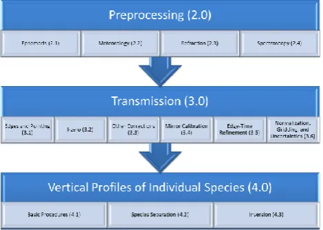
Slant-path transmission profiles are converted into optical depths and then combined with spectroscopy data to separate into species-specific slant-path optical depth profiles. These are then inverted to produce vertical profiles of ozone (O3), nitrogen dioxide (NO2), water vapor (H2O), and aerosol ex-tinction (at 1020, 525, 452, and 386 nm) using a simple onion-peeling technique. In order to do this, the inversion algorithm must make the assumption that the layer of atmo-sphere at each altitude is homogeneous, or at least has a con-stant gradient, through the whole swath that the instrument observes. This assumption has obvious limitations in the tro-posphere and well-understood biases at higher altitudes for certain species due to rapid photochemistry, giving rise to a nonlinear variation across the terminator (Chu and Cunnold, 1994), but works well through most of the stratosphere (Cun-nold et al., 1989). A general outline of the algorithm can be seen in Fig. 1. The sections that follow provide greater de-tail on the various steps just outlined and note when and how these differ from the approach of SAGE II version 6.2.
2 Preprocessing
Before anything can be done with the solar irradiance data measured by the instrument, a series of preprocessing steps must be performed so that this data can be placed in the proper context. The algorithm needs to determine where the instrument was looking during the collection of each data packet. This requires processing spacecraft orbital ephemeris data, along with atmospheric refraction information and the requisite meteorological information. In addition, some cal-culations related to the spectroscopy of the instrument are performed to facilitate later calculations.
2.1 Ephemeris
Fig. 1: A general outline of the SAGE II algorithm. The numbers correspond to sections in this paper.
Fig. 1. A general outline of the SAGE II algorithm. The numbers correspond to sections in this paper.
than 61◦ or events that occur during spacecraft viewed so-lar eclipses are excluded from further processing. High beta angles are excluded because the duration of an event (and subsequent ground track) becomes long and the assumption of atmospheric spherical symmetry, used for the inversion process, breaks down. For each remaining event, the original spacecraft state vectors just prior to the start of the event are used as input to the processing algorithm. Using a model for Earth’s gravitational potential, the equations of motion are calculated and the state vectors are propagated throughout the event. In addition to the state vectors, the position of the Sun is calculated for each time. Then, for each time, coordi-nate and geometrical data required by the algorithm are cal-culated. This includes information related to the spacecraft (sub-spacecraft latitude, longitude, and altitude), the Sun (an-gular size, right-ascension, declination, and azimuth), and the tangent point (altitude, latitude, longitude) looking at the cen-ter, top, and bottom of the Sun.
The methodologies for these calculations originate from Buglia (1988). For the most part, these methods are straight-forward geometry but, in pre-version 7.0 algorithms, some aspects (e.g., sidereal time, precession, nutation, and Sun po-sition) were approximated using numerical constants derived from pre-1984 data. It is important to note that in 1984, na-tional and internana-tional almanacs adopted a revised set of physical constants put forth by the International Astronom-ical Union in 1976, which necessitated a change to vari-ous numerical constants used in these approximations. How-ever, these changes were not uniformly implemented and data quality in versions prior to version 7.0 was adversely impacted by an inconsistency in ephemeris epoch usage.
In version 7.0, all physical constants (e.g., Earth’s equa-torial and polar radii and gravitational constant) have been updated to those used in the World Geodetic System 1984 (WGS84, updated in 2004) (NIMA Technical Report, 1997), which is the current standard. The constants used for the
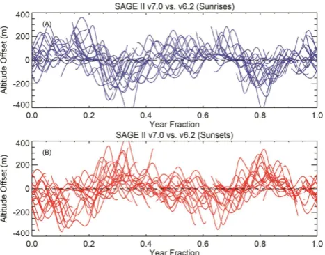
Toolkit routine has corrected what was a previously unknown quasi-random error in the altitude registration in the SAGE II data products. For any given event, this correction manifests itself as an altitude offset between SAGE II versions 6.2 and 7.0. This altitude offset can be positive or negative, can have a magnitude up to a few hundred meters, and varies from event to event. While there is no simple dependence upon beta angle or latitude, there is some correlation with time of year, as expected, as shown in Fig. 2.
2.2 Meteorology
SAGE processing algorithms require ancillary meteorolog-ical data that relates density and temperature to altitude. SAGE II version 6.2 used multiple sources of data to yield density and temperature data (i.e.,P/T data) from the surface up to 100 km. NCEP reanalysis data (Kalnay et al., 1996) was used first, yieldingP/T data from 1000 mbar up to 10 mbar (∼30 km). Above that, operational model data provided by NCEP was used up to 0.4 mbar (∼50 km). Lastly, the Global Reference Atmospheric Model-1995 (GRAM-95) (Johnson et al., 1995) was used to extend the profiles up to 100 km. Since each atmospheric layer is assumed to be uniform, a sin-gle location was chosen to retrieveP/T data from, namely, the 20 km subtangent latitude and longitude. The temperature and pressure data sets were then combined and interpolated to a standard 0.5 km-spaced altitude grid.
Fig. 2: Tangent height registration differences between version 7.0 and 6.2 for the same time index near a tangent height of 60 km for sunrises/sunsets (top/bottom) as a function of time of year. A single point is plotted for each SAGE II event.
Fig. 2. Tangent height registration differences between version 7.0 and 6.2 for the same time index near a tangent height of 60 km for sunrises/sunsets (top/bottom) as a function of time of year. A single point is plotted for each SAGE II event.
MERRA data for the reprocessing of SAGE III/M3M data to the version 7.0 standard and to use operational GEOS data for the upcoming SAGE III/ISS mission. SAGE II version 7.0 uses MERRA data from the surface up to 0.1 mbar and GRAM-95 above that up to 100 km. Instead of using the ac-tual GRAM-95 temperature values, the GRAM-95 lapse rate is used to extrapolate above the MERRA data. This is done because the MERRA lower mesospheric temperature values are often smaller than those from GRAM-95. Any attempt to merge the two data sets can introduce an artificial inversion layer in the lower mesosphere.
In both versions, afterP/T profiles are determined, num-ber density profiles are calculated. In order to have uncer-tainty estimates in derived quantities in the inversion process (e.g., uncertainty estimates for Rayleigh scattering slant-path extinction), we calculate an uncertainty estimate in this den-sity calculation, based on the uncertainty in the original tem-perature data. NCEP reanalysis does not provide uncertainty estimates for their model products; however, we obtained some temperature uncertainty values (ranging from 4 K in the troposphere to 15 K in the mesosphere) to use at each pressure level (Finger et al., 1993). MERRA also does not provide uncertainty estimates for their model products. We continue to discuss the topic of model uncertainties with the MERRA group. In the meantime, we are currently adapting the NCEP uncertainty values as a rough guideline.
2.3 Refraction
Our refraction algorithm calculates the elevation angle (rel-ative to the local horizontal plane at the position of the spacecraft) of the refracted Sun (where the instrument sees the Sun) and the total refraction angle of the light ray as a
Fig. 3: Coincident event temperature profile comparisons between SAGE III and SAGE II. The biases in the middle stratosphere between SAGE III and SAGE II v6.2 data are unexplained. The comparison with v7.0 illustrates differences in the shape of the upper stratosphere between MERRA and NCEP/GRAM-95, with MERRA typically having a less well-defined transition to the mesosphere and a cooler and/or higher (in altitude) stratopause.
Fig. 3. Coincident event temperature profile comparisons between SAGE III and SAGE II. The biases in the middle stratosphere between SAGE III and SAGE II v6.2 data are unexplained. The comparison with v7.0 illustrates differences in the shape of the upper stratosphere between MERRA and NCEP/GRAM-95, with MERRA typically having a less well-defined transition to the meso-sphere and a cooler and/or higher (in altitude) stratopause.
function of wavelength and possible tangent heights assum-ing spherical geometry (Fig. 4). It also calculates the layer slant-path matrix with which it determines the total number density of the slant-path air column (mass path) by integrat-ing along the curved path of the light ray (again with a spher-ical model). The use of a spherspher-ical model for these calcula-tions provides a good first guess before refinement using an oblate Earth model can be done. These parameters are chosen because, for each packet, the algorithm needs to know pre-cisely where on the Sun the instrument is pointing and these parameters allow it to easily go between where the instru-ment is pointing in space and where the instruinstru-ment is look-ing on the face of the Sun. The methodology of computation remains largely unchanged from version 6.2 and comes from Chu (1983) and Auer and Standish (2000). After refraction, tangent point altitudes, latitudes, and longitudes are updated, taking an oblate Earth model into account.
Fig. 4: SAGE refracted viewing geometry.
Fig. 4. SAGE refracted viewing geometry.
range, and would be interpreted as non-physical characteris-tics in the atmosphere, which could propagate downward in the inversion process. However, while this potentially intro-duced random deviations in derived products (e.g., as large as a few percent in ozone), the effect averaged out, even within a single event, to zero. As such, correcting this error in version 7.0 did not uncover or correct any biases in prior versions. 2.4 Spectroscopy
The retrieval process requires absorption cross-sections for O3, NO2, the oxygen dimer (O2-O2), and molecular (Rayleigh) scattering at all wavelengths. This is done by first combining each channel’s measured spectral response function with the solar spectrum (Kurucz et al., 1984). The spectral response of channels 2, 5, and 6 also incor-porate the long-term evolution in the spectral characteris-tics of their respective band-pass filters. These spectral re-sponses are then combined with cross-section data for each species (i.e., O3, NO2, O2-O2, and Rayleigh) and integrated across each channel’s spectral range. Rayleigh cross-sections (cm2molecule−1) are wavelength-dependent and are calcu-lated in the same fashion as in Bucholtz (1995). O2-O2 cross-sections (cm5molecule−2) are taken to be wavelength-dependent, are assumed to scale with density, and are cal-culated in the same fashion as Mlawer et al. (1998) (for wavelengths encompassing channels 1 and 2) and Newnham and Ballard (1998) (for wavelengths encompassing channels 3 through 7). O3and NO2cross-sections (cm2molecule−1) are taken to be both wavelength-dependent and temperature-dependent. In version 6.2, they were derived from the Shet-tle and Anderson cross-section compilation (ShetShet-tle and Anderson, 1995), which is the same cross-section compila-tion that was used in SAGE III version 3.0. In SAGE III version 4.0 (Thomason et al., 2010), however, the O3 cross-sections were updated to the Bogumil (Scanning Imag-ing Absorption Spectrometer for Atmospheric Chartogra-phy (SCIAMACHY) V3) cross-sections (Bogumil et al., 2003), which had a positive impact on several data products
Fig. 5: Absorption cross-sections for SAGE II retrieved species at 250 K over SAGE II measurement wavelengths for v7.0.
Fig. 5. Absorption cross-sections for SAGE II retrieved species at 250 K over SAGE II measurement wavelengths for v7.0.
and produced better agreement with in-atmosphere measure-ments (Pitts et al., 2006). As such, SAGE II version 7.0 uses the SCIAMACHY V3 O3cross-sections, including compan-ion measurements of NO2absorption cross-sections encom-passing SAGE II measurement wavelengths (Fig. 5). These band-pass averaged, or effective, cross-sections are com-bined with vertical density (for O2-O2)or temperature pro-files (for O3and NO2)to create vertical “profiles” of effec-tive cross-sections for these species in each channel, facili-tating later computations.
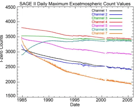
Fig. 6: Daily maximum exoatmospheric “I-zero” count values for each channel. While a general degradation in response can be seen in each channel over time, a few channels, namely 2, 6, and 7, went through periods of rapid change during the beginning of the mission.
Fig. 6. Daily maximum exoatmospheric “I zero” count values for each channel. While a general degradation in response can be seen in each channel over time, a few channels, namely 2, 6, and 7, went through periods of rapid change during the beginning of the mis-sion.
line data for version 6.2 were provided by L. Brown (per-sonal communication, 2002), which were later incorporated into the water vapor line data for the 2004 version of the HITRAN (high resolution transmission) molecular spectro-scopic database (Rothman et al., 2004). The version 7.0 wa-ter vapor line data come from the 2008 version of HITRAN (including the 2009 update to water vapor) (Rothman et al., 2009). These line data are used to precompute derivatives of absorption as a function of temperature, pressure, and line-of-sight molecular number density for later use with an emissivity curve-of-growth approximation (EGA) as the for-ward model for water vapor absorption (Gordley and Russell, 1980).
After SAGE II had been operating for some time, a long-term analysis of the water vapor product showed it to be in poor agreement with other satellites and ground measure-ments. While many possibilities were considered, and even-tually ruled out, it was determined that the poor quality of water vapor data was a result of a shift in the spectral re-sponse of the water vapor channel (channel 2) prior to 1986 (Fig. 6). The primary reason behind this thinking was an in-cident associated with the SAGE II instrument during one of its final thermal vacuum tests just prior to being shipped off for integration with the ERBS. An incomplete shutdown of the cooling system caused condensation within the instru-ment. It is believed that the channel filters absorbed water and then subsequently dried out on orbit, affecting their spectral characteristics. Unfortunately, it was impossible to reproduce this in the lab as no original filter material remained and the company that created it was no longer in business. Version 6.2 was the first version to attempt to account for an apparent shift in the location of the water vapor channel filter. In order
Fig. 7: SAGE II v6.1/v6.2 (top/bottom) water vapor data (dots) and HALOE climatological data (lines). (Thomason et al., 2004) Fig. 7. SAGE II v6.1/v6.2 (top/bottom) water vapor data (dots) and
HALOE climatological data (lines) (Thomason et al., 2004).
to attempt to model the filter characteristics, it was decided to adjust the spectral response of the water vapor channel to make the mean SAGE II water vapor data at one latitude and season agree with a HALOE (UARS (Upper Atmosphere Re-search Satellite) Halogen Occultation Experiment) (Russell et al., 1993) climatological profile for the same latitude and season (northern mid-latitudes in March). The center wave-length and full-width at half-max (FWHM) were adjusted and the two data sets were again compared. While it was im-possible to completely match these data sets, it was found that the best match came from a center wavelength shift of +10 nm (945 nm) and an increase in the FWHM of 10 % (22 nm). This was then applied to all SAGE II data from 1986 onward. The before and after comparisons of that work can be seen in Fig. 7. (Thomason et al., 2004)
Fig. 8: SCIAMACHY V3 O3 cross-sections minus the Shettle and Anderson compilation at 250 K in the range of 930-970 nm.
Fig. 8. SCIAMACHY V3 O3cross-sections minus the Shettle and Anderson compilation at 250 K in the range of 930–970 nm.
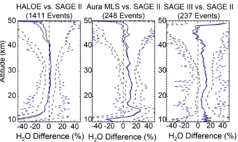
to the details of ozone (Chu et al., 1993), the evolution of the water vapor channel spectral response was reevalu-ated. A comparison of SAGE II version 6.2 with newer data sets (Fig. 9) shows that, while version 6.2 matches well to HALOE, as expected, there is an offset of about 10 % with both SAGE III and the MLS (Microwave Limb Sounder) (Lambert et al., 2007) on board the Aura satellite, perhaps suggesting the choice of HALOE as a standard for inferring channel drift was not optimal. The channel 2 drift assessment was repeated, except SAGE III water vapor was used to infer the location of the water vapor channel rather than HALOE. The smallest difference between data sets came from an addi-tional center wavelength shift of+2.7 nm (947.7 nm) and an additional increase in the FWHM of 5 % (23 nm). An updated set of instrument-to-instrument comparisons can be seen in Fig. 10.
SAGE II is able to measure NO2 by observing the dif-ference in absorption between the two channels located at 452 nm (channel 5) and 448 nm (channel 6). Another look at exoatmospheric data (Fig. 6) shows that, like the water vapor channel, channel 6 may have had a change in spec-tral response prior to 1990 as a result of the aforementioned thermal vacuum testing incident. We chose a similar, but slightly different approach, to that used to correct the wa-ter vapor channel. Since NO2measurements are derived pri-marily from the differential extinction between the two chan-nels, we chose to use one channel to calibrate the other, since the long-term variation in solarI zero showed channel 5 to be well behaved. The differential effective cross-sections be-tween the two channels were compared to the differences in their exoatmospheric counts. It was assumed that any differ-ence in the exoatmospheric counts of channel 6 relative to that seen in channel 5 over time were a result of a change in the band-pass of its filter. In this way, a time-dependent fit could be made that allowed the application of a differential cross-section correction to the effective cross-sections in
Fig. 9: A comparison of HALOE/Aura MLS/SAGE III minus SAGE II v6.2 water vapor products over their coincident events (<2° lat, <10° lon, <2.5 hr.). For each plot, mean data are shown in black while median data are shown in blue (uncertainties are shown with dashed lines). Since HALOE was used to infer channel drift in v6.2, they are obviously in good agreement. However, there is an offset of about 10% with both Aura MLS and SAGE III.
Fig. 9. A comparison of HALOE/Aura MLS/SAGE III minus SAGE II v6.2 water vapor products over their coincident events (< 2◦lat, < 10◦lon, < 2.5 h). For each plot, mean data are shown in black while median data are shown in blue (uncertainties are shown with dashed lines). Since HALOE was used to infer channel drift in v6.2, they are obviously in good agreement. However, there is an offset of about 10 % with both Aura MLS and SAGE III.
channel 5 to obtain the effective cross-sections in channel 6 for any time during the mission. The time-dependent model for the channel 6 spectral band-pass required the determina-tion of the initial properties and the rate of change relative to the observed long-term anomalousI zero drift. To compute these, the SAGE II NO2 stratospheric column abundances were compared to twilight NO2 measurements at Lauder, New Zealand (Johnston and McKenzie, 1984). This proce-dure was applied in version 6.2, though only at one temper-ature (240 K). The dependence of SAGE II NO2retrieval on O3necessitated a repeat of this procedure after both the O3 and NO2cross-section databases were changed. The differ-ence in version 7.0 is the implementation of a temperature-dependent differential cross-section correction and the use of SAGE III NO2data to determine the starting spectral location of channel 6. The overall quality of SAGE II NO2 measure-ments relative to the SAGE III NO2measurements remains mostly unchanged between versions (Fig. 11).
3 Transmission
The transmission algorithm combines measured limb-darkening curves with timing and pointing data to produce slant-path optical depths for each tangent altitude between 0.5 km and 100 km in 0.5 km increments. In order to do this, a number of physical and instrumental sources of variation must be compensated for.
Fig. 10: A comparison of HALOE/Aura MLS/SAGE III minus SAGE II v7.0 water vapor products over their coincident events (<2° lat, <10° lon, <2.5 hr.). For each plot, mean data are shown in black while median data are shown in blue (uncertainties are shown with dashed lines). This shows the SAGE II v7.0 water vapor product to be in much better agreement with Aura MLS and SAGE III data sets than v6.2.
Fig. 10. A comparison of HALOE/Aura MLS/SAGE III minus SAGE II v7.0 water vapor products over their coincident events (< 2◦lat, < 10◦lon, < 2.5 h). For each plot, mean data are shown in black while median data are shown in blue (uncertainties are shown with dashed lines). This shows the SAGE II v7.0 water vapor prod-uct to be in much better agreement with Aura MLS and SAGE III data sets than v6.2.
Fig. 11: SAGE III NO2 minus SAGE II v6.2/v7.0 (left/right) over coincident events (<2° lat,
<10° lon, <2.5 hr.). The overall quality of SAGE II NO2 remains mostly the same between
versions. The bias above 38 km is a source of ongoing study.
Fig. 11. SAGE III NO2minus SAGE II v6.2/v7.0 (left/right) over coincident events (< 2◦lat, < 10◦lon, < 2.5 h). The overall quality of SAGE II NO2remains mostly the same between versions. The bias above 38 km is a source of ongoing study.
information (Sect. 3.1) to place each data packet on the face of the Sun, followed by computing a preliminary I zero (Sect. 3.2). From this, a preliminary transmission is cre-ated (avoiding sunspots) and the mirror calibration is com-puted (avoiding PMCs and accounting for Rayleigh scatter-ing) (Sect. 3.4). TheI zero curves are then updated (includ-ing a correction for the electronic transient (Sect. 3.3) if the event is a sunset). OnceI zero curves have been obtained, a refined estimate of transmission is computed. The edge-time refinement algorithm (Sect. 3.5) is iterated for convergence to improve the point registration on the face of the Sun and
Fig. 12: Solar irradiance data measured by SAGE II for a typical sunset event showing both exoatmospheric and in-atmosphere scans. The shortening of scan duration as a function of flattening of the Sun due to refraction can clearly be seen. The alternating duration of each scan is a byproduct of spacecraft and orbital motions. Typically for sunset events, scans that move from the bottom to the top of the Sun (“up” scans) take less time than scans that move from the top to the bottom of the Sun (“down” scans).
Fig. 12. Solar irradiance data measured by SAGE II for a typi-cal sunset event showing both exoatmospheric and in-atmosphere scans. The shortening of scan duration as a function of flattening of the Sun due to refraction can clearly be seen. The alternating dura-tion of each scan is a byproduct of spacecraft and orbital modura-tions. Typically for sunset events, scans that move from the bottom to the top of the Sun (“up” scans) take less time than scans that move from the top to the bottom of the Sun (“down” scans).
a resultant transmission profile is computed (Sect. 3.6). If the event is a sunrise, the electronic transient correction is computed and applied. Lastly, a time-dependentI zero cor-rection is performed and the entire process is reiterated so that the algorithm can take advantage of every correction available. The algorithm then proceeds to resample the trans-mission data to the standard grid and compute uncertainties (Sect. 3.6).
3.1 Edges and pointing
The first step in transmission processing requires that the limb-darkening curves (Fig. 12) be combined with pointing data to place every data packet accurately on the face of the Sun. First the limb-darkening curves in the 1020 nm chan-nel are used to determine where the physical top and bot-tom edges of the Sun are by looking for the inflection points and the times associated with them. The timing of science packet data and ephemeris pointing data can then be accu-rately mapped to each other. This mapping is done by as-suming that the rate of motion of the scan-mirror is constant during a scan so that each packet of data within a scan can be interpolated to a location on the face of the Sun.
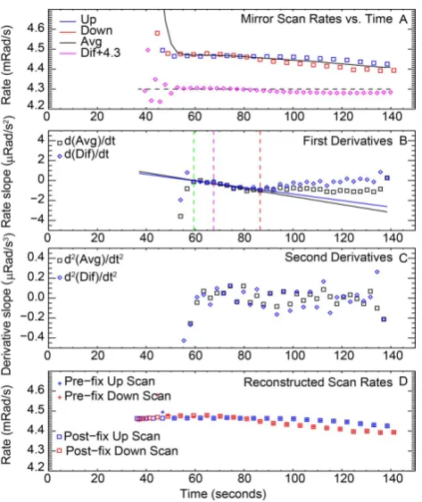
Fig. 13: Scan-mirror rate data for a sunrise event. Fits to the first derivatives of the average scan rate and difference between up and down scan rates are used to reconstruct scan rate data at low altitudes where scan rate data have gone bad. Only the scans just above where rate data go bad are used (between the green and red dashed lines in plot B). To avoid any programmatic errors with using the second derivative data to determine where rates have gone bad, an altitude upper limit of 60 km is used (dashed purple line). The comparison between original and reconstructed scan rates is shown in plot D.
Fig. 13. Scan-mirror rate data for a sunrise event. Fits to the first derivatives of the average scan rate and difference between up and down scan rates are used to reconstruct scan rate data at low alti-tudes where scan rate data have gone bad. Only the scans just above where rate data go bad are used (between the green and red dashed lines in (B). To avoid any programmatic errors with using the second derivative data to determine where rates have gone bad, an altitude upper limit of 60 km is used (dashed purple line). The comparison between original and reconstructed scan rates is shown in (D).
the scan-mirror itself and the orbital and attitudinal motions of the spacecraft. A look at the average scan rates and the dif-ference between up and down scan rates for a typical event shows that they are generally well behaved and slowly vary-ing with time (Fig. 13a). The derivatives of these quantities show linearity with respect to time (Fig. 13b). However, at any time during the event, the attitude actuators on the space-craft (these keep the spacespace-craft in a desired orientation) can turn on or off and cause an abrupt shift in these derivatives. While attitude control maneuvers do not affect retrieved scan rates due to the fact that they affect the retrieved top and bottom edge times equally, they do account for the kink in Fig. 13b. The linearity of derivatives with respect to time al-lows for a fit of these quantities to data just above where the rate data begins to go bad, which is characterized by large values in the first or second derivatives (Fig. 13c). These fits are then used to reconstruct low altitude rate data (Fig. 13d) in order to compensate for scans with bad edge calculations resulting from the bottom of the Sun being occluded by cloud or the limb of the Earth.
determining the tangent point altitude was determined to be better than 20 meters. Lower in the atmosphere (in the tropo-sphere), where refraction effects can become large, the un-certainty in the tangent point altitude is dominated by uncer-tainties in the meteorological data. Each packet of data, in each channel, is subsequently assigned a time, tangent alti-tude, position on the face of the Sun, scan-mirror elevation position, and photodiode count value.
3.2 Izero
In order to create transmission profiles, the algorithm cal-culates ratio measurements made by the instrument looking at a particular point on the Sun through the atmosphere to the same point seen above the atmosphere. Thus one of the first things the transmission algorithm does is create a stan-dard exoatmospheric limb-darkening curve (Izero curve) ra-tio measurement to map other scans to. The instrument gen-erally collects between 10 and 20 exoatmospheric scans, so these are combined into a pair ofI zero curves, one for up-scans and one for down-up-scans, which are then interpolated to a fine grid in position on the face of the Sun (∼1000 points in version 7.0 versus∼100 points in version 6.2). As the I zero curve is mapped onto each scan (including the exoatmospheric or I zero scans), an edge time refinement (see Sect. 3.5) is made for theI zero scans. A new addition in version 7.0 is the introduction of a time-dependentI zero correction, which was first introduced in SAGE III version 4.0. A time-dependent I zero correction benefits high alti-tude scans by helping to correct for apparent rotation of the scan track across the face of the Sun due to orbital motions (Burton et al., 2010).
required the user to manually screen them out (Wang et al., 2002). In version 7.0, all events without a minimum num-ber ofI zero scans are dropped from processing and flagged accordingly.
3.3 Other corrections
Once anI zero curve is established (and mapped to each scan), a preliminary transmission can be computed for each scan. This then allows the calculation of a few corrections that need to be made. An initial correction for Rayleigh at-tenuation is done (for the benefit of other corrections) and a polar mesospheric cloud (PMC) detection routine is run (Burton and Thomason, 2000). While no overall correction is made in the presence of PMCs, the use of data within PMCs will be avoided when determining the mirror calibration (see Sect. 3.4). A sunspot detection routine is also run and mea-surements inside of sunspots are flagged so that they can be filtered later. It was found that the sunspot detection routine in version 6.2 would often overcompensate in its sunspot fil-tering (i.e., it would often omit all data from the start of a sunspot to the edge of the Sun) and a more robust algorithm has been introduced for version 7.0, which identifies sunspots by their characteristic shapes in both the first and second derivatives of the limb-darkening curves. In order to avoid false positives resulting from noise in the limb-darkening curves, the derivatives are normalized and the magnitude and shape of both derivatives are used simultaneously to identify sunspots.
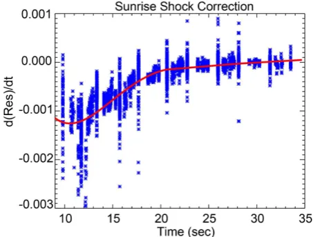
As the SAGE II instrument began taking data during each event, a small transient was observed in channels 5 and 6. This so-called thermal shock needed to be accounted for in the data processing. For sunset events, this is relatively easy as the data are fairly homogenous (exoatmospheric scans) and any time dependency is easily recognized and removed. For sunrise events, however, the transient occurs while the instrument is looking through the attenuated atmosphere and the correction is necessarily at low altitudes. In this case, scan-to-scan variations in the channel 5 and 6 differential extinction at a given altitude, which are correlated in time across multiple scans, are examined. By looking at the ratio of channel 6 to channel 5, which is used for the NO2retrieval, the algorithm determines the rate of change of differential extinction, which is then integrated to produce a correction that is applied to these two channels (Fig. 14). The impact on the transmission in these channels is on the order of 0.25 %, whereas the impact on other channels (were it to be applied) would be no more than 0.05 % (SPARC/IOC/GAW, 1998).
3.4 Mirror calibration
SAGE operates by using a scan-mirror to move the instru-ment field-of-view up and down across the solar disk (normal to the Earth’s limb). The reflectivity of the scan-mirror varies slightly with the angle of incidence and requires calibration.
Fig. 14: The sunrise shock correction fits the differential extinction between channels 5 and 6 with an exponential and computes the residuals. The residuals within an altitude bin are then analyzed, computing the rate of change of the residuals as a function of time. The blue asterisks in the plot denote the computed derivatives while the red line denotes the fit. Once computed, this fit is integrated to derive a correction factor to apply to the originally computed differential extinctions.
Fig. 14. The sunrise shock correction fits the differential extinction between channels 5 and 6 with an exponential and computes the residuals. The residuals within an altitude bin are then analyzed, computing the rate of change of the residuals as a function of time. The blue asterisks in the plot denote the computed derivatives while the red line denotes the fit. Once computed, this fit is integrated to derive a correction factor to apply to the originally computed differential extinctions.
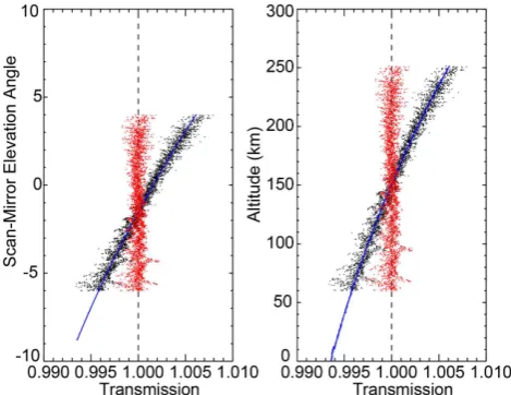
This is not an absolute reflectance calibration as only the rel-ative change in reflectivity with angle is required. In version 6.2, this calibration was determined through a quadratic fit to exoatmospheric transmission data as a function of alti-tude and was performed only once at the end of transmission processing. In version 7.0, this quadratic fit is to exoatmo-spheric transmission data as a function of the elevation angle of the scan-mirror and is performed in the overall iterations of transmission processing. In each case, the mirror calibra-tion is applied as a multiplicative correccalibra-tion to remove cur-vature in the high altitude transmission data, which should theoretically be a constant value of 1 with some instrument noise. Since smaller angles (higher altitudes) are used for the fit, an extrapolation of the correction term to larger an-gles (lower altitudes) is necessary to correct attenuated data. An example of the mirror correction can be seen in Fig. 15, demonstrating that the angular dependence of the reflectivity of the scan-mirror is on the order of 0.5 %.
3.5 Edge-time refinement
The edge-time refinement algorithm is designed to minimize any biases in the limb-darkening curves created by slight er-rors of the initial calculation of the edge times of each scan. The measured solar intensity of a scan (I) in a given channel (λ)is a function of both position on the face of the Sun (p) and altitude (z), which are themselves both functions of time (t), and can be written as
Fig. 15: SAGE II v7.0 mirror correction for the 452 nm channel on the very first iteration of a sunset event. The correction is a quadratic fit to raw high-altitude transmission as a function of scan-mirror elevation angle. The black dots show the raw transmission values and the blue line shows the correction factor. The corrected transmission (red dots) are raw transmission divided by the correction factor. The plot on the left shows transmission data points and correction factors versus scan-mirror elevation angle while the plot on the right shows the same points plotted against the corresponding altitude. The correction factors are extrapolated outside of the range of the fitted transmission data points for use with low altitude transmission data. Fig. 15. SAGE II v7.0 mirror correction for the 452 nm channel on the very first iteration of a sunset event. The correction is a quadratic fit to raw high-altitude transmission as a function of scan-mirror el-evation angle. The black dots show the raw transmission values and the blue line shows the correction factor. The corrected transmission (red dots) are raw transmission divided by the correction factor. The plot on the left shows transmission data points and correction fac-tors versus scan-mirror elevation angle while the plot on the right shows the same points plotted against the corresponding altitude. The correction factors are extrapolated outside of the range of the fitted transmission data points for use with low altitude transmission data.
whereI0is theI zero limb-darkening curve,T is the slant-path transmission, andεis the error in the measurements or estimates. Since there is some inherent uncertainty in the cal-culated edge times, Eq. (1) can realistically be rewritten as
I (λ, p (t+εt) , z (t+εt))=I0(λ, p (t )) T (λ, z (t ))
+ε (λ, p (t ) , z (t )) , (2) whereεt is related to uncertainties in the edge times. There
are two cases that can be considered separately. The first case is for high altitude measurements whereT (z)=1, and Eq. (2) can be expanded into
I (λ, p (t+εt))=I λ, p+εp
=I0(λ, p)+
dI0(λ, p) dp εp
=I0(λ, p)+
dI0(λ, p)
dp (c1+c2p) , (3)
whereI0is the estimate for theIzero curve andc1andc2are the linear shift and stretch coefficients, respectively. The cor-rection is a linear function because position on the face of the Sun is linearly mapped to time. The derivative term is calcu-lated using finite differences and a multiple linear regression technique is used to obtain the shift and stretch terms, which yield the correction to the edge times.
The second case involves measurements in the atmosphere whereT (z)can no longer be ignored. In this case, Eq. (2) can
1 2
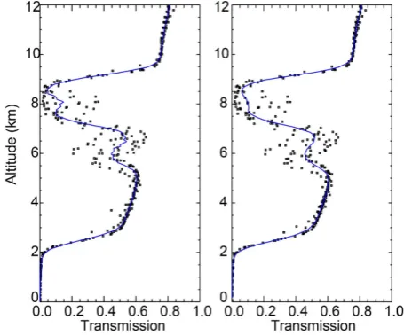
coefficients. Following the same procedure, the correction to the edge times is obtained. Since the pair of edge times apply equally to all spectral channels, the derivatives are performed at each wavelength and used together in the regression cal-culation. The shift and stretch algorithm has the effect of re-moving spectrally and vertically correlated noise in the trans-mission profile, typically at low altitudes (Fig. 16).
3.6 Normalization, gridding, and uncertainties
Fig. 16: The effect of the shift and stretch algorithm on 1020 nm transmission during the first iteration for two separate SAGE II events. The black marks/lines denote pre-S&S transmission (shifted to the left by 0.2 in transmission for ease of viewing) while the blue marks/lines denote post-S&S transmission. The shift and stretch algorithm helps to remove a lot of the noise associated with inaccurate edge times.
Fig. 16. The effect of the shift and stretch (S&S) algorithm on 1020 nm transmission during the first iteration for two separate SAGE II events. The black marks/lines denote pre-S&S transmis-sion (shifted to the left by 0.2 in transmistransmis-sion for ease of viewing) while the blue marks/lines denote post-S&S transmission. The shift and stretch algorithm helps to remove a lot of the noise associated with inaccurate edge times.
in the Sun’s photosphere (e.g., granulation) combined with the apparent rotation of the solar disk during the event, as op-posed to instrumental noise. These variations manifest them-selves as low amplitude oscillatory patterns in high altitude transmission (on the order of 0.1 %) that are periodic in al-titude (due to their high correlation with surface features on the Sun) and correlated between channels (Fig. 18). An ex-tension of the time-dependentI zero algorithm to compen-sate for this effect is in development. Lastly, all slant-path transmission profiles are converted to slant-path optical depth profiles.
4 Vertical profiles of individual species
The inversion algorithm takes slant-path optical depth pro-files and, along with other data such as P/T data, sepa-rates them into species-specific slant-path optical depth pro-files before finally inverting them into vertical propro-files of O3 and NO2 number densities, H2O volume mixing ratio, and aerosol extinction. While much of this follows the same ba-sic procedure described in Chu et al. (1989), there are some important differences between versions 6.2 and 7.0, some of which include more subtle aspects of the algorithm. As such, this section will generally review the entire inversion process. The uncertainties throughout this process are prop-agated from uncertainties in the neutral density and derived transmission profiles.
Fig. 17: The normalization and fitting process for most iterations (left) and the final iteration (right) of the algorithm. Black marks denote transmission values for each packet while the blue lines denote the fitting process.
Fig. 17. The normalization and fitting process for most iterations (left) and the final iteration (right) of the algorithm. Black marks denote transmission values for each packet while the blue lines de-note the fitting process.
4.1 Basic procedures
The viewing geometry of SAGE is such that at each tangent height the instrument looks through the atmosphere, it is also looking through a slant-path column of air that incorporates all of the tangent heights above it. Accounting for refraction, a triangular path-length matrix is computed. The slant-path total column at each tangent height, derived from a matrix multiplication of the path-length matrix and density profile, is thus comprised of the sum of partial slant-path columns from all overlying 0.5 km thick layers. This simple matrix operation allows for an “onion peeling” process to be per-formed later for inverting a species’ slant-path optical depth profile to the species density profile.
The first step in the retrieval of vertical profiles of indi-vidual species is to account for and remove the contributions of molecular (Rayleigh) scattering in all channels and O2 -O2absorption in a subset of channels. O2-O2cross-sections (cm5molecule−1) are scaled with density and both O2-O2 and Rayleigh effective cross-sections (cm5molecule−2) are combined with the path total column to convert to slant-path optical depths, which are then subtracted from each channel. The largest source of uncertainty in the retrieved profiles of individual species comes from uncertainty in the contribution from molecular scattering, which itself origi-nates from uncertainty in the temperature profile.
4.2 Species separation
Fig. 18: The plots on the left show the creation of an I-zero curve for both up (top) and down (bottom) scans. Each I-zero curve (black line) is created from multiple exoatmospheric scans (red marks). These plots are zoomed in on the center 20% of the scan/Sun to show how there are both minor variations in intensity across the face of the Sun as well as some inherent uncertainty in the resulting value of the I-zero curve. The plots in the middle show normalized up (top) and down (bottom) I-zero curves for each channel to show how these spatial variations are strongly correlated across channels (channels 1-7 are discernible from outermost to innermost). It is very likely that this variation is representative of physical variation on the Sun (e.g. solar granulation). The plot on the right shows high altitude transmission for several channels. The repetitive oscillatory patterns that are strongly correlated between channels are the direct result of this unfiltered physical variation. For now, this is not compensated for in the final transmission profiles but, as a new feature in version 7.0, is accounted for in the uncertainty estimates.
Fig. 18. The plots on the left show the creation of anI zero curve for both up (top) and down (bottom) scans. EachI zero curve (black line) is created from multiple exoatmospheric scans (red marks). These plots are zoomed in on the center 20 % of the Sun scan to show how there are both minor variations in intensity across the face of the Sun as well as some inherent uncertainty in the resulting value of theIzero curve. The plots in the middle show normalized up (top) and down (bottom)Izero curves for each channel to show how these spatial variations are strongly correlated across channels (channels 1–7 are discernible from outermost to innermost). It is very likely that this variation is representative of physical variation on the Sun (e.g., solar granulation). The plot on the right shows high altitude transmission for several channels. The repetitive oscillatory patterns that are strongly correlated between channels are the direct result of this unfiltered physical variation. For now, this is not compensated for in the final transmission profiles but, as a new feature in version 7.0, is accounted for in the uncertainty estimates.
altitudes in which all five channels are available, and alti-tudes above which it is believed there is no aerosol extinction. These five channels are used because the poor quality of the 386 nm channel prevents its use in the broad retrieval. Sig-nificant absorption by water vapor occurs only in the 940 nm channel and is inverted in a separate process.
The first step is to find the highest extent to which one of the five channels is not available (i.e., no valid or non-fill data) and begin just above that. The residual slant-path opti-cal depth (hereafter abbreviated as OD) in each channel con-sists of contributions from O3, NO2, and aerosol, though at longer wavelengths (particularly 1020 nm) the contribution from gas species absorption becomes vanishingly small. At this point we have measurements with seven unknowns: O3, NO2, and aerosol at each wavelength. We solve this set of equations using a least-squares solution where we approxi-mate the aerosol contribution at 600 and 448 nm as the linear combination of aerosol at 1020, 525, and 452 nm. The full set of species separation equations to be solved can be expressed as
c1(λi)ODAer(λ1)+ σO3(λi)
σO3(λ3)
ODO3(λ3)+c2(λi)ODAer(λ4)
+c3(λi)ODAer(λ5)+
σNO2(λi)
σNO2(λ5)
ODNO2(λ5)=OD(λi)
wherei= {1,3,4,5,6}is the channel number,σ (λi)is the
effective cross-section of the stated species at the given chan-nel, OD (λi)is the slant-path optical depth of the stated
chan-nel, and the channel specific aerosol, O3, and NO2ODs are
the unknowns. Most of the coefficients for this process (c1, c2, andc3)are simply “1s” and “0s” (e.g., for channels 1, 4, and 5), and those that are not are determined using an en-semble of single mode log-normal size distributions of sul-fate aerosol at stratospheric temperatures, though, in practice, composition is of secondary importance. The ensemble of log-normal size distributions spans the observed wavelength-dependence of the aerosol spectra and is used to estimate the relative dependence of extinction in channels 3 and 6 as a function of the values in channels 1, 4, and 5. The ensem-ble consists of a large range of mode radii and widths that effectively span the observed relationships of the dependent and independent aerosol channels. Ultimately this is simply a means of interpolating between nominal aerosol channels as, given the log-normal ensemble extinction estimates at 1020, 525, and 452 nm, the range of values possible at 600 or 448 nm is small. Using simple linear processes, the coeffi-cients that relate the dependent extinction values to the three independent extinction values are robust, and residuals of the fit provide at least some information regarding uncertainty in clearing aerosol from each channel.
OD is calculated as a residual. This process separates the var-ious species from lower altitudes (typically in the middle to upper troposphere) up to some maximum altitude (typically set to 75 km).
While this retrieval works very well, it typically suffers from attempting to retrieve species at higher altitudes where extinction values are near detection limits and noise becomes the dominant signal. This noise is a carryover of the channel-correlated solar structure noise first discussed in Sect. 3.6, which does not dampen at higher altitudes. Much of this noise ends up being interpreted by the algorithm as aerosol and detrimentally affects the simultaneous retrieval of all species. To compensate for this in version 6.2, a separate re-trieval scheme was used that uses only 4 channels (600, 525, 452, and 448 nm) and assumes that no aerosol is present to calculate O3OD in the 600 nm channel and NO2OD in the 448 nm channel. Water vapor was again treated as a residual in the 940 nm channel. In lieu of more adaptive methods, this process began at 40 km up to some maximum altitude (typ-ically 75 km). Thereafter, the 5-channel retrieval was transi-tioned into the “no aerosol” retrieval between 40 and 45 km. The version 7.0 algorithm utilizes the data to determine how to transition into regions where the inclusion of aerosol in the retrieval is no longer necessary, the methods of which are outlined later in this section.
For altitudes below the 5-channel retrieval, there is no longer valid data in the 448 nm channel and thus NO2 can-not be simultaneously retrieved. Instead, the NO2OD profile from the 5-channel retrieval is inverted to get extinction val-ues and the algorithm reconstructs ODs at lower altitudes by assuming the NO2 mixing ratio is zero. The OD contribu-tion from NO2at lower altitudes is then removed from all channels. With NO2 removed, the algorithm begins work-ing from the bottom of the 5-channel retrieval and moves down. It first uses a 4-channel retrieval (1020, 600, 525, and 452 nm) so long as there is valid data and then transitions to a 3-channel retrieval (1020, 600, and 525 nm) when necessary. The main retrieval algorithm stops if there is no longer any valid data in any of these three channels. Aerosol extinction in the 1020 nm channel is thereafter retrieved until no further data exists. These data are then used to estimate the contri-bution of aerosol in the 940 nm channel so that water vapor can again be calculated as a residual.
This entire process goes through two iterations. The first iteration uses a default set of weighting coefficients to de-termine the contribution of aerosol at 600 and 448 nm. In the second iteration, we use the measured 525 to 1020 nm aerosol extinction ratio to select sets of coefficients deter-mined using the fits to the ensemble of aerosol spectra for values around the observed value. This accounts for a small degree of nonlinearity observed in the fits to 600 and 448 nm aerosol extinction. In reality, this is a distinctly second order correction but seems to reduce the sensitivity of the quality of the ozone data product to aerosol, particularly when aerosol levels are high. However, for the same reasons that version
6.2 has a “no aerosol” retrieval, at altitudes near and above 40 km, the 525 to 1020 aerosol OD ratio can begin to vary wildly through non-physical numbers. This has a detrimental effect on the second iteration retrievals, producing extremely “noisy” data above 35 km. In version 7.0, once the retrieved aerosol OD in each channel drops below a predetermined threshold, a nonlinear least squares fit is made to the data in the form of an exponential decay curve. Above the alti-tude where these fits drop below the amplialti-tude of the noise, the fits are used for the 525 to 1020 ratio instead of the ac-tual data. The second iteration retrievals then have far more realistic weighting coefficients to work from.
While the use of fits to determine the 525 to 1020 ratio does improve the quality of the 5-channel retrievals, partic-ularly above 35 km, it can still suffer from the same limi-tations that necessitated the use of a “no aerosol” retrieval above 40 km, namely the fact that the aerosol ODs at higher altitudes can still become non-physical and detrimentally af-fect the simultaneous retrieval of all species. Typically this is a byproduct of retrieved non-physical aerosol OD values in the shorter wavelengths at higher altitudes detrimentally im-pacting the retrieved values in longer wavelengths. This had the tendency (in version 6.2) to result in O3and NO2values that were biased high at altitudes above∼40 km. To compen-sate for this, in version 7.00, the algorithm looks only at the 600 nm channel to retrieve ozone in these altitude regimes. When the fit to the 600 nm aerosol OD drops below a cer-tain threshold, the algorithm subtracts out the fit (which is generally below the “noise level”) and inverts only the re-maining 600 nm OD to retrieve ozone. A more adaptive al-gorithm is being developed for retrieving NO2at higher al-titudes though, for now, the high bias persists from version 6.2.
Fig. 19: Coincident event mean water vapor mixing ratio profiles between SAGE III (blue) and SAGE II (black) (v6.2 left and v7.0 right). In v6.2, SAGE II water vapor mixing ratio profiles tended to asymptote towards large values near the top of the retrieval, a trait that SAGE III v4.0 also exhibits. In v7.0, this has been corrected. The overall change in bias between v6.2 and v7.0 comes from a change in ozone spectroscopy and a modification of the water vapor channel filter response towards results in better agreement with SAGE III and Aura MLS.
Fig. 19. Coincident event mean water vapor mixing ratio profiles between SAGE III (blue) and SAGE II (black) (v6.2 left and v7.0 right). In v6.2, SAGE II water vapor mixing ratio profiles ap-proached asymptote towards large values near the top of the re-trieval, a trait that SAGE III v4.0 also exhibits. In v7.0, this has been corrected. The overall change in bias between v6.2 and v7.0 comes from a change in ozone spectroscopy and a modification of the wa-ter vapor channel filwa-ter response towards results in betwa-ter agreement with SAGE III and Aura MLS.
4.3 Inversion
After species separation, water vapor is the first retrieved species. The slant-path optical depth data are first converted to extinction and then smoothed to help mitigate noise in the weak signal. The algorithm to retrieve water vapor mixing ratio remains mostly unchanged from Chu et al. (1993) with one small exception. Originally the process began at 50 km and worked down. The algorithm requires a small range of al-titude at the top of the retrieval process to establish the abun-dance and scale height of the H2O profile as a boundary con-dition. Improvements in the version 7.0 transmission allow the starting altitude to be moved up to 60 km. This, combined with the aforementioned aerosol fit method, has greatly im-proved the water vapor product above 40 km. In version 6.2, water vapor mixing ratio profiles would suffer from a char-acteristic “hook” towards unrealistically large values nearing 50 km. This can also be seen in SAGE III version 4.0 water vapor mixing ratio profiles. With these modifications to the retrieval, this “hook” has been removed (Fig. 19).
Prior to version 7.0, once water vapor was retrieved at the end of the first iteration, its contribution to the 600 nm chan-nel was removed and the second iteration began. This had an inconsequential impact on ozone above the hygropause. However, below the hygropause, SAGE II ozone retrievals have consistently been biased low when compared with other data (Wang et al., 2002). This feature was turned off in
mains is to invert the O3and various aerosol slant-path col-umn optical depth profiles into vertical extinction profiles. As with NO2, the O3vertical extinction profile is then con-verted to a vertical number density profile by simply divid-ing by the effective cross-section. The inversion technique used in version 7.0 is different from that used in version 6.2, which utilized Twomey’s modification of Chahine’s al-gorithm (Chahine, 1972; Twomey, 1975) to retrieve extinc-tion values and a simple onion-peeling technique to retrieve uncertainty estimates. The Twomey–Chahine algorithm was found to have several undesirable behaviors. It would not al-low negative values and therefore introduced a positive bias in regions of the density (extinction) profile where the signal-to-noise ratio was small, typically at the higher altitude end of the retrieved profile. It also systematically approached the solution from one direction and stopped once the tolerance criterion was met, producing another form of bias as a result. Lastly, its use introduced discontinuities in the profile when the slant-path extinction fell below a preset value and verti-cal smoothing was activated. Given the high quality of the SAGE II version 7.0 transmission profiles and the algorith-mic limitations of the Twomey–Chahine inversion method, it was replaced entirely with onion-peeling in version 7.0.
Lastly, with all primary data products computed, the aerosol extinction in the 525 and 1020 nm channels are used to compute some physical parameters to characterize aerosol at each altitude. The methods outlined in Thomason et al. (2008) are used to determine the effective radius and surface area density of aerosol particles.
5 Results of version 7.0
This paper describes the SAGE II version 6.2 and version 7.0 algorithms. Prior versions of SAGE II data products have been well validated (e.g., Wang et al., 2002) and included in numerous international assessments (e.g., WMO, 2011). Several of the version 7.0 changes affect the quality of these data products and a brief assessment of the differences seen in the version 7.0 data products follows.
5.1 Event comparisons
almost entirely from the change in spectroscopy, resulting in a nearly uniform decrease in concentration of∼1.5 % in the stratosphere. The magnitude of the offset increases to about 2 % above 40 km due to the removal of the “no aerosol” method of retrieval. The large increase in ozone below 10 km is a result of the removal of the water vapor correction to ozone. The difference between the mean and median below 20 km is a result of using onion-peeling for inversion instead of Twomey–Chahine, as the outliers in version 6.2 were bi-ased positive whereas in version 7.0 they can take on nega-tive values, though overall the same number of outliers exist. While the changes move SAGE II ozone values further from SAGE III concentrations by about 1.5 % despite using the same spectroscopy, the changes in the retrieval method make the offset vary less with altitude.
Given the diurnal nature of NO2, sunrise and sunset events are compared separately. Figure 21, left and middle panels, show comparison plots for sunset and sunrise NO2, respec-tively. Due to changes in spectroscopy, the overall concen-tration of sunset NO2 has dropped by 5–10 % in the mid-stratosphere. The large decrease below 20 km is again a re-sult of using onion-peeling instead of Twomey–Chahine for inversion. As previously mentioned, sunset NO2values are biased high above 40 km and an algorithm to better retrieve NO2at these higher altitudes is in development. Net changes in sunrise NO2 are an amalgamation of changes made in transmission, spectroscopy, species separation, and inver-sion. Sunrise NO2remains somewhat of a research product as quantifying the impact on sunrise NO2data quality is ham-pered by the fact that insufficient high quality sunrise NO2 measurements exist for comparison during the time period where SAGE II measured sunrise NO2(all comparisons with SAGE III are sunset events due to power problems late in the mission, forcing operation at half duty cycle). Looking at the sunset/sunrise NO2ratio, however, reveals that the data are more consistent in the mid-stratosphere in version 7.0 than in version 6.2 (Fig. 21 right panel).
While no changes have been made to the retrieval of aerosol extinction in version 7.0 specifically, the data in various channels are impacted by the changes made to the spectroscopy and the technique used for inversion (Fig. 22). As a result of using onion-peeling instead of Twomey– Chahine for inversion, aerosol extinction tends to decrease more quickly at higher altitudes, as opposed to asymptot-ing to some positive non-zero value as in previous versions. The overall data quality through the mid-stratosphere has re-mained mostly unchanged for aerosol extinction in the 1020 and 385 nm channels. The change in spectroscopy has had a large impact on the comparisons between SAGE II and SAGE III aerosol extinction in the 525 and 452 nm chan-nels. SAGE II version 7.0 aerosol extinction at 525 nm is in much better agreement with SAGE III version 4.0 as compared to SAGE II version 6.2, whereas the opposite is true for aerosol extinction at 452 nm. We have transitioned the aerosol derived products including surface area density
Fig. 20: Comparison plots of ozone. The figure on the left shows SAGE II v7.0 minus v6.2 for all events excluding the time period of heavy aerosol interference from the Mount Pinatubo eruption. The other two figures show SAGE III v4.0 minus SAGE II v6.2/v7.0 (middle/right) over their coincident events. The comparison of each of SAGE III’s main ozone data products is shown. MLR ozone (retrieved by a multiple linear regression technique) is represented in blue while aerosol ozone (retrieved in a fashion similar to SAGE II) is represented in red. Fig. 20. Comparison plots of ozone. The panel on the left shows SAGE II v7.0 minus v6.2 for all events, excluding the time period of heavy aerosol interference from the Mount Pinatubo eruption. The other two panels show SAGE III v4.0 minus SAGE II v6.2 and v7.0 (middle and right, respectively) over their coincident events. The comparison of each of SAGE III’s main ozone data products is shown. MLR ozone (retrieved by a multiple linear regression tech-nique) is represented in blue while aerosol ozone (retrieved in a fashion similar to SAGE II) is represented in red.
(SAD) and effective radius (Reff) from the technique out-lined in Thomason et al. (1997) to a more robust method developed in Thomason et al. (2008). Since there is some concern about the newer technique’s performance at low 525 to 1020 nm aerosol extinction coefficient levels, the new op-erational method transitions from the 2008 method for ratios above 2.0 to the old method for ratios below 1.5 with a linear mix in between. As a result, aerosol products do not change significantly during the post-Pinatubo period but change sub-stantially during the clean period, particularly after 1998. The change in this period can be seen in Fig. 23 where the SAD has increased by 50 % throughout the lower stratosphere and theReffhas decreased by about 10 %.
Fig. 21: Comparison plots of NO2. The plots at the left/middle show SAGE II v7.0 sunset/sunrise NO2 minus SAGE II v6.2 sunset/sunrise NO2 for all events excluding the time period of heavy aerosol interference from the Mount Pinatubo eruption. The plot on the right shows the mean NO2 sunset over sunrise ratio for all events (again excluding Pinatubo) in the tropics for v6.2 (black) and v7.0 (blue). Results are similar in other latitude bands.
Fig. 21. Comparison plots of NO2. The plots at the left and mid-dle show SAGE II v7.0 sunset and sunrise NO2, respectively, mi-nus SAGE II v6.2 sunset and sunrise NO2, respectively, for all events, excluding the time period of heavy aerosol interference from the Mount Pinatubo eruption. The plot on the right shows the mean NO2sunset over sunrise ratio for all events (again excluding Pinatubo) in the tropics for v6.2 (black) and v7.0 (blue). Results are similar in other latitude bands.
of the channel. However, removing the remaining “ozone-like” signal from water vapor required nearly doubling the FWHM of the channel. It is well understood that some level of uncertainty exists in laboratory experiments to retrieve temperature-dependent ozone absorption cross-sections, par-ticularly in the Wulf bands (Bogumil et al., 2003). Since the release of the SCIAMACHY V3 ozone cross-section database, several other ozone cross-section databases have been released that show significant changes in the Wulf bands relative to the Chappius (e.g., Chehade et al., 2013; Serdyuchenko et al., 2011). While we are hesitant to adopt a new cross-section database until it has been validated, SAGE II data suggests that the relative ozone spectroscopy in the SCIAMACHY V3 database could be off by on the or-der of 10 %. We have identified many possible combinations of changing both the filter location and the relative ozone spectroscopy in order to minimize differences with SAGE III water vapor. However, any change to the ozone spectroscopy creates a coupled problem when comparisons are made with SAGE III water vapor, as the same spectroscopy would have to be adopted by SAGE III as well. As it currently stands, the water vapor product in SAGE II version 7.0 is in much bet-ter agreement with SAGE III version 4.0 than was SAGE II version 6.2. However, we are still not satisfied with the result and this issue remains a topic of further study.
5.2 Time series analysis
Herein we present a new way of fitting SAGE II data for use with time series analysis; namely, we fit the entirety of the data at a single altitude simultaneously using the dates and latitudes of the measurements as they were made (i.e., no
Fig. 22: Comparison plots of aerosol extinction. The figure on the left shows SAGE II v7.0 minus v6.2 for all events. The other two figures show SAGE III v4.0 minus SAGE II v6.2/v7.0 (middle/right) over their coincident events.
Fig. 22. Comparison plots of aerosol extinction. The panel on the left shows SAGE II v7.0 minus v6.2 for all events. The other two panels show SAGE III v4.0 minus SAGE II v6.2 and v7.0 (middle and right, respectively) over their coincident events.
Fig. 23: Comparison plots of aerosol derived products. The figure on the left shows SAGE II aerosol surface area density in v7.0 minus v6.2 for all events after and including 1998. The figure on the right shows SAGE II aerosol effective radius in v7.0 minus v6.2 for all events after and including 1998.
Fig. 23. Comparison plots of aerosol derived products. The panel on the left shows SAGE II aerosol surface area density in v7.0 minus v6.2 for all events after and including 1998. The panel on the right shows SAGE II aerosol effective radius in v7.0 minus v6.2 for all events after and including 1998.
latitude gridding or monthly means). The purpose of this fit was for the creation of climatologies, but has revealed some interesting data quality impacts between versions 6.2 and 7.0. Since the content of this paper focuses on the residuals of the fit rather than the fits themselves, we will only briefly outline the fitting process.
The fitting process begins by applying a modification of the Wang et al. (2002) filtering criteria to each event and then taking daily (zonal) means of collocated events. The follow-ing functional form is then regressed to all of the data:
Fig. 24: Left – SAGE III and SAGE II mean water vapor mixing ratio profiles over all coincident events after shifting the water vapor channel center wavelength +12.0 nm. Right – SAGE III minus SAGE II water vapor comparison over coincident events after adjusting the water vapor channel in various ways: A – center wavelength +12.0 nm, FWHM +50%; B – center wavelength +11.5 nm, FWHM +40%, ozone effective cross-section in water vapor channel artificially decreased by 10%; C – center wavelength +11.3 nm, FWHM +45%, ozone cross-section database changed to Serdyuchenko (2011); D – center wavelength +12.7 nm, FWHM +15% (channel location prior to inclusion of MERRA in SAGE II v7.0).
Fig. 24. Left – SAGE III and SAGE II mean water vapor mixing ratio profiles over all coincident events after shifting the water va-por channel center wavelength+12.0 nm. Right – SAGE III mi-nus SAGE II water vapor comparison over coincident events af-ter adjusting the waaf-ter vapor channel in various ways: A – cen-ter wavelength+12.0 nm, FWHM+50 %; B – center wavelength +11.5 nm, FWHM+40 %, ozone effective cross-section in water vapor channel artificially decreased by 10 %; C – center wavelength +11.3 nm, FWHM+45 %, ozone cross-section database changed to Serdyuchenko et al. (2011); D – center wavelength+12.7 nm, FWHM+15 % (channel location prior to inclusion of MERRA in SAGE II v7.0).
whereηis the concentration of the given species (i.e., O3, NO2, and H2O),2(θ )is the functional form of the latitudi-nal dependence, andT (t )is the functional form of the time dependence.2(θ )is simply a Fourier series (6 harmonics) with the constraint of zero derivative at the poles.T (t ) con-tains semiannual (3, 4, and 6 month terms), annual, quasi-biennial oscillation (QBO) (Singapore wind proxy at 30 hPa and 50 hPa), solar cycle (11 yr period terms), and equiva-lent effective stratospheric chlorine (EESC) (Newman et al., 2007) (for fits to O3)terms as well as an additional piece-wise term to account for any potential diurnal variation in a species. Both 2(θ )andT (t )also contain a constant term, which collectively provide the constant for the fit. Residual analysis is performed to omit any outliers with large influ-ence on the data and a correction is made for lag-1 autocor-relation (Reinsel et al., 1981). This fit is performe