Determination of circumsolar radiation from Meteosat Second Generation

www.atmos-meas-tech.net/7/823/2014/ doi:10.5194/amt-7-823-2014

© Author(s) 2014. CC Attribution 3.0 License.

Atmospheric

Measurement

Techniques

Determination of circumsolar radiation from Meteosat Second

Generation

B. Reinhardt1, R. Buras2, L. Bugliaro1, S. Wilbert3, and B. Mayer2

1_{Deutsches Zentrum für Luft- und Raumfahrt e.V., Institut für Physik der Atmosphäre, Oberpfaffenhofen, Germany} 2_{Meteorologisches Institut München, Ludwig-Maximilians-Universität, Munich, Germany}

3_{Deutsches Zentrum für Luft- und Raumfahrt e.V., Institute of Solar Research, Plataforma Solar de Almería (PSA),}

Tabernas, Spain

Correspondence to: B. Reinhardt (bernhard.reinhardt@dlr.de)

Received: 24 April 2013 – Published in Atmos. Meas. Tech. Discuss.: 25 June 2013 Revised: 16 October 2013 – Accepted: 17 December 2013 – Published: 31 March 2014

Abstract. Reliable data on circumsolar radiation, which is caused by scattering of sunlight by cloud or aerosol parti-cles, is becoming more and more important for the resource assessment and design of concentrating solar technologies (CSTs). However, measuring circumsolar radiation is de-manding and only very limited data sets are available. As a step to bridge this gap, a method was developed which al-lows for determination of circumsolar radiation from cirrus cloud properties retrieved by the geostationary satellites of the Meteosat Second Generation (MSG) family. The method takes output from the COCS algorithm to generate a cirrus mask from MSG data and then uses the retrieval algorithm APICS to obtain the optical thickness and the effective ra-dius of the detected cirrus, which in turn are used to deter-mine the circumsolar radiation from a pre-calculated look-up table. The look-up table was generated from extensive cal-culations using a specifically adjusted version of the Monte Carlo radiative transfer model MYSTIC and by developing a fast yet precise parameterization. APICS was also improved such that it determines the surface albedo, which is needed for the cloud property retrieval, in a self-consistent way in-stead of using external data. Furthermore, it was extended to consider new ice particle shapes to allow for an uncertainty analysis concerning this parameter.

We found that the nescience of the ice particle shape leads to an uncertainty of up to 50 %. A validation with 1 yr of ground-based measurements shows, however, that the frequency distribution of the circumsolar radiation can be well characterized with typical ice particle shape mixtures, which feature either smooth or severely roughened particle

surfaces. However, when comparing instantaneous values, timing and amplitude errors become evident. For the circum-solar ratio (CSR) this is reflected in a mean absolute devia-tion (MAD) of 0.11 for both employed particle shape mix-tures, and a bias of 4 and 11 %, for the mixture with smooth and roughend particles, respectively. If measurements with sub-scale cumulus clouds within the relevant satellite pix-els are manually excluded, the instantaneous agreement be-tween satellite and ground measurements improves. For a 2-monthly time series, for which a manual screening of all-sky images was performed, MAD values of 0.08 and 0.07 were obtained for the two employed ice particle mixtures, respec-tively.

1 Introduction

angular distance from the Sun. The steepness and shape of this angular gradient depends on the particles’ type, shape and size as well as on the optical thickness. Thus, percep-tion of circumsolar radiapercep-tion by any optics pointed at the Sun is strongly dependent not only on its opening half-angleα

but also on the sky conditions. Such optics can be a pyrhe-liometer withα=2.5◦(World Meteorological Organization standard according to CIMO Guide, 2008, Chap. 7) but, for example, also a concentrating solar thermal power plant with

α <1◦. Furthermore, the discrepancy in perception caused by different opening angles is not constant and also varies with sky conditions. Since circumsolar radiation is com-monly included in direct normal irradiance (DNI) measure-ments at higher amounts than perceived by CST plants, this can lead to systematic overestimation of the solar resource when DNI alone is available.

There has been some effort to measure circumsolar radi-ation from the ground (e.g. Noring et al., 1991; Neumann et al., 2002; DeVore et al., 2009; Wilbert et al., 2011, 2013) and also to simulate it for a range of atmospheric conditions (e.g. Thomalla et al., 1983). So far, however, circumsolar radiation has not been determined from satellite measure-ments, which have large advantages considering global cov-erage, site intra-comparability and financial costs compared to ground measurements. Moreover, satellite data are readily available for many regions of the world and covering longer time spans than most available ground measurement time se-ries of circumsolar radiation. In this study a method is devel-oped to derive the circumsolar radiation utilizing the Spin-ning Enhanced Visible and Infrared Imager (SEVIRI) aboard the geostationary Meteosat Second Generation (MSG) satel-lites (Schmetz et al., 2002).

The focus of this study lies on circumsolar radiation caused by cirrus clouds with an optical thicknessτ ranging from 0.1 to 3.0. Clouds in this optical thickness range affect radiation, but still allow for the operation of CSTs; however they are also detectable by satellites. Cirrus clouds typically occur in this range, while water clouds usually exhibit an op-tical thickness too large to allow for the operation of CSTs.

The presented method to derive the circumsolar radiation comprises two steps. First the particle size and optical thick-ness of the cirrus clouds are determined using the Algo-rithm for the Physical Investigation of Clouds with SEVIRI (APICS) (Bugliaro et al., 2011, 2012, 2013). A parameteri-zation is then applied to convert these cloud properties into circumsolar radiation. We developed this parameterization based on simulations of the sunshape with an improved ver-sion of the radiative transfer solver “Monte Carlo Code for the Physically Correct Tracing of Photons in Cloudy Atmo-spheres”, MYSTIC (Mayer, 2009).

The manuscript is structured as follows. In Sect. 2, basic definitions are made. The problems and solutions with re-spect to the exact simulation of the sunshape with MYSTIC are described. Furthermore the difficulties of retrieving prop-erties of thin cirrus clouds with APICS and respective

improvements are outlined. Finally, the parameterization of the circumsolar radiation is developed. In Sect. 3, we ap-ply the method to 1 yr of SEVIRI data processed through APICS and study the impact of the ice particle shape that so far cannot be determined from MSG. The results are also compared to ground measurements of the circumsolar ratio (CSR) performed at the Plataforma Solar de Almería (PSA) with the measurement system presented by Wilbert et al. (2013). A conclusion is given in Sect. 4.

2 Material and methods

2.1 Sunshape and circumsolar ratio

The one-dimensional radiance distribution along a radial cut outwards from the Sun’s centre is called sunshape. The cir-cumsolar ratio (CSR) is a common scalar quantity that can be used to characterize the sunshape (Buie et al., 2003). It is defined as the normal irradiance coming from an annular region around the Sun divided by the normal irradiance from this circumsolar region and the sun disk. For the remainder of the document the term irradiance always refers to normal irradiance, i.e. irradiance on a surface perpendicular to the direction pointing at the Sun.

The disk angleαsungives the extent of the sun disk

mea-sured from its centre to the edge. The circumsolar region reaches from the Sun’s edge to the angleαcir(> αsun), which

is subject to arbitrary definition and measured from the Sun’s centre as well. With this we can write

CSR(αcir)=

R2π

0

Rαcir

αsunL(α)cos(α)sin(α)dαdφ R2π

0

Rαcir

0 L(α)cos(α)sin(α)dαdφ

, (1)

whereLis the sunshape – i.e. the radiance depending on the angular distanceαfrom the Sun’s centre. The cosine term is safely neglected in our calculations, as even for the maximum

αcir of 5◦considered in this study, the errors due to this are

smaller than 0.2 %.

2.2 Radiative transfer modelling

The parameterization for the circumsolar radiation that is de-veloped in the following is based on extensive simulations of the sunshape under different atmospheric conditions. Let us therefore briefly consider the radiative transfer code MYS-TIC and how it was improved to allow for an exact simulation of the sunshape.

The scattering phase function of ice crystals exhibits a strong forward peak. This may cause rare but result-dominating events – so-called “spikes”. Levelling the spikes increases computing time excessively. A solution for this problem was given recently by Buras and Mayer (2011). The variance reduction methods described in this publication are implemented in MYSTIC. It is therefore well suited to simu-late the radiance distribution in the circumsolar region.

To simplify the radiative transfer, the Sun is commonly as-sumed to be a point source at infinite distance. All sunrays are therefore parallel and enter the atmosphere under the same angle. However this approximation is not appropriate when simulating radiance in the vicinity of the sun disk since the Sun has a finite angular extent. Furthermore the centre of the sun disk is brighter than the limb. This so-called limb darkening is caused by absorption in the Sun’s atmosphere and is therefore wavelength-dependent. To take account of these effects, a sun disk source was implemented in MYSTIC which uses the wavelength-dependent limb-darkening model as given in Scheffler and Elsässer (1990) and Köpke et al. (2001). This disk source is used in the simulation of the dif-fuse, as in the simulation of the direct radiation.

All simulations in the following neglect the temporal course of the Sun’s angular radiusαsunand refer to a mean

angular sun radius of 0.266◦. From reference simulations we estimate that the absolute error in CSR that arises from this is less than±0.004 as long asαcir>0.375◦. However,

as Neumann et al. (2002) demonstrated, it is important that the integration limit αsun in Eq. (1) is consistent with the

Sun’s radius, or otherwise larger errors will arise. Therefore, the Sun’s actual radius according to the Sun–Earth distance should be taken into account in Eq. (1) when calculating CSR from real ground-based sunshape measurements.

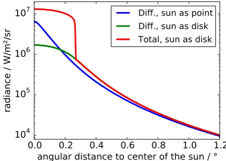
The model extensions are illustrated in Fig. 1. The dif-ferences between a simulation of the diffuse radiance with a point source (blue) and a sun disk source (green) are pro-nounced for angles smaller than≈1◦from the Sun’s centre, which is in line with findings by Grassl (1971). The red curve shows the total sunshape consisting of direct and diffuse ra-diation.

2.3 Optical properties of cirrus clouds

Passive satellite instruments with only one viewing direction do not provide information about the ice particle shape com-position within a cloud, which therefore has to be assumed a priori. The particle shape influences the optical proper-ties of the cloud, such as the scattering phase function and the single-scattering albedo. This in turn influences both the cloud property retrieval and the modelling of the circumsolar radiation. To assess the uncertainty that is caused by the as-sumption of the ice particle shape, we use several cloud bulk optical properties for modelling the circumsolar radiation, as well as for the cloud property retrieval with APICS.

0.0 0.2 0.4 0.6 0.8 1.0 1.2

angular distance to center of the sun / °

10

10

10

10

radiance / W/m²/sr

Diff., sun as point

Diff., sun as disk

Total, sun as disk

Fig. 1. Simulated broadband sunshape (integrated solar) for a

cir-rus cloud with optical thickness 0.5 and with the Sun in the zenith. Blue: diffuse radiance for a point source. Green: diffuse radiance for a disk source. Red: direct and diffuse radiance for a disk source. Optical properties for a cirrus composed of HEY solid columns (see Sect. 2.3) with an effective radius of 40 µm were employed in the simulations.

The effective radiusreff is a parameter that is commonly

used to characterize the scattering and absorption properties of disperse particle size distributions by means of a single scalar (Hansen and Travis, 1974; McFarquhar and Heyms-field, 1998). For spherical particles like water droplets it is defined as the ratio of the third to the second moment of the size distribution. There is, however, an ambiguity in the def-inition ofrefffor non-spherical particles. We stick to the

def-inition that was used in the generation of the bulk optical properties (e.g. Baum et al., 2005a):

reff=

3RV (D)n(D)dD

4RA(D)n(D)dD, (2)

wherenis the number concentration, D the maximum di-mension,V the volume andAthe projected area of the par-ticles.

2.4 Remote sensing of ice clouds with APICS and its optimization for optically thin clouds

This study relies on the APICS framework to derive effec-tive radius and optical thickness of the cirrus clouds. APICS (Bugliaro et al., 2011, 2012, 2013) implements a cloud prop-erty retrieval based on the work of Nakajima and King (1990) for SEVIRI channels 1 and 3 in the solar spectrum (centred at 0.6 and 1.6 µm). APICS was originally developed as a multi-purpose cloud property retrieval. However for this study it is of special importance that optically thin cirrus clouds are re-trieved with as little error as possible. To account for that, we modified APICS as described in the following.

The retrieval is only performed for pixels classified as cir-rus. While APICS originally relied on a cirrus cloud mask generated by the Meteosat Second Generation Cirrus Detec-tion Algorithm v2 (MeCiDa) (Krebs et al., 2007; Ewald et al., 2013), we produced cloud masks based on the algorithm “Cloud Optical properties derived from CALIOP and SE-VIRI” (COCS) (Kox et al., 2011; Kox, 2012) since it detects more of the optically thin cirrus. Ostler (2011) and Bugliaro et al. (2012) compared the detection efficiency of COCS and MeCiDa utilizing airborne high-spectral-resolution lidar (HSRL) observations. They found that both algorithms de-tect virtually all of the cirrus clouds withτ >0.5, but COCS has advantages at smaller optical thickness: while MeCiDa detects about 50 % of the cirrus clouds withτ≈0.2, COCS shows a higher detection efficiency of over 80 %. COCS uses a neural network approach to convert the brightness temper-ature information from the infrared channels of SEVIRI into the parameters ice optical thickness and cloud-top pressure. The neural network was trained with a collocated data set of SEVIRI observations and retrieval results for the CALIOP lidar, which is onboard the polar-orbiting satellite CALIPSO (Winker et al., 2009). As mentioned, the output of COCS is not a cloud flag per se, but an optical thickness value. To generate a cloud mask, all pixels that are assigned an optical thickness larger than 0.1 by COCS are assumed to be cloudy.

This cut-off criterion ofτ >0.1 is necessary to keep the false alarm rate at an acceptable level (S. Kox, personal communi-cation, 2012).

For the operation of APICS in this study it was assumed that channels 1 and 3 of the SEVIRI instrument aboard the “Meteosat 9” MSG satellite exhibit an underestimation of about 6 % (Ham and Sohn, 2010) and an overestimation of 2 %, respectively (P. Watts, EUMETSAT, personal com-munication, 2009). A preprocessing step takes care of the corresponding recalibration of reflectance values. Recently, Meirink et al. (2013) published similar calibration coeffi-cients. In a satellite inter-calibration study they found an un-derestimation of 8 % and an overestimation of 3.5 % for the SEVIRI channels 1 and 3, respectively.

The APICS retrieval uses look-up tables (LUTs) in which pre-simulated reflectivity values for the two SEVIRI chan-nels are stored as a function of the most relevant parameters, namely as a function of the sun and satellite zenith angles, the relative azimuth between the Sun and satellite, the albedo in both channels, the particle size in terms of the effective radius and the optical thickness. Simplifications and assump-tions about the state of the atmosphere are required because the two independent pieces of information (the two satellite channels) only allow for the retrieval of two quantities, in our case optical thickness and effective radius.

The most important sources of uncertainty concerning thin ice clouds are the assumptions about the ground reflectivity, aerosol beneath the clouds and the ice particle shape. While we have no solution for the latter, we adapted APICS such that errors in the cloud property retrieval due to wrong as-sumptions of the ground reflectivity and long-term aerosol variability are reduced. This is outlined in the following.

APICS relies on an albedo value to describe the ground reflectivity. It must be determined a priori for both SE-VIRI channels at every pixel. The original version of APICS used albedo products based on measurements of the Moder-ate Resolution Imaging Spectroradiometer (MODIS) aboard polar-orbiting satellites – either the “blacksky” or “whitesky” albedo from the Ambrals processing scheme (Strahler et al., 1999). During this study APICS was modified so that it gen-erates its own self-consistent albedo product. This product is based on the SEVIRI clear-sky reflectance map, which is the average of the reflectance for a given time of day over the seven preceding days under clear-sky conditions (EUM OPS DOC 09 5165, 2011). The clear-sky reflectance con-tains contributions from the ground as well as from the atmo-sphere. From this combined signal the ground albedo needs to be extracted. The albedo values in both SEVIRI chan-nels are therefore retrieved using the APICS LUTs. To this end it is evaluated for which albedo the psimulated re-flectivity values match the clear-sky reflectance best, where

albedo also corrects for some of the long-term variability in the aerosol properties, which may deviate from the constant aerosol properties assumed in the simulations for the APICS LUTs.

The clear-sky reflectance map is routinely only available for 12:00 UTC. Therefore the albedo is only retrieved at this time and assumed to be constant during the day. The success rates (defined in the following) reached by APICS with this method are superior when compared to using the MODIS albedo data sets.

The cloud property retrieval results can be erroneous because of the uncertainties in the assumptions described above, and because of other shortcomings (e.g. 1-D radiative transfer calculations). Often the measured reflectivity pair cannot even be reproduced by any parameter combination in the LUT. In these cases the retrieval will return the maximal or minimal values ofτorrefffrom the LUT such that the

dif-ference between the measured and pre-simulated reflectivity combination is minimized. We call these occurrences “out-liers”. This definition of “outlier” is very strict. In principle one could add all those data points to the “hits”, which lie within the uncertainty range of the retrieval due to errors in the measurements and in the assumptions. These errors are, however, difficult to quantify. Since we use the number of outliers only as a relative quality criterion, the exact defini-tion is not relevant. The success rateSof the cloud property retrieval is defined as 1 minus the ratio of the number of out-liers to the total number of considered pixels in a domain:

S=1− number of outliers

number of considered pixels. (3) The success rate was calculated within a test sector (lo-cation shown in Fig. 5) for four months meant to represent the four different seasons (June 2011, September 2011, De-cember 2011 and March 2012). The averages over these four months for the MODIS blacksky, the MODIS whitesky and the APICS-generated albedo are 62, 62 and 81 %, respec-tively, when using the Baum v2.0 optical properties. Con-sidering the better results with the APICS-generated albedo, APICS was operated with this new albedo product for the re-trieval of circumsolar radiation. Note that success means the retrieval obtained values covered by the LUT, which, how-ever, still need not be correct. In the following, all retrieval results are considered, successful or not, because they have an inherent uncertainty and even the outliers are the best pos-sible result for the given set of measurements.

One can conclude from the imperfect success rate of 81 % that this approach of generating a self-consistent sur-face albedo alleviates the problems with wrong a priori as-sumptions, but does not solve them completely. The APICS-generated albedo product can adapt to changes of the real surface albedo only on the scale of a few days, while real changes can occur on the scale of hours. Further reading on the influence of an inhomogeneous surface albedo on

Nakajima and King-like cloud property retrievals can be found in Fricke et al. (2012).

Bugliaro et al. (2013) examined the APICS optical thick-ness especially for optically thin cirrus clouds also utilizing the airborne HSRL measurements. In their study the Baum and HEY bulk optical properties were used as well. In gen-eral APICS delivered larger optical thickness values than the HSRL. In a linear regression, slopes of 1.26 and 1.54 were found for Baum v2.0 and Baum v3.5, respectively. The cor-relation coefficient is close to 0.8 for all optical property data sets. However, only approximately 150 data pairs could be used in their study. They all belong to the same flight that was conducted under low-sun conditions (θsunapproaching 80◦),

which poses a challenge for the APICS cloud property re-trieval. Furthermore Bugliaro et al. (2013) used a similar, but not completely identical, method to derive the ground albedo from SEVIRI measurements as in this study.

2.5 Parametrization of circumsolar radiation

In this section a way of efficiently parameterizing the CSR is developed. We thereby build on the concept of an apparent optical thickness. We also evaluate the uncertainty of the pa-rameterization under the fact that the ice particle shape can-not be retrieved from MSG.

As mentioned previously, the circumsolar radiation rele-vant for CST applications is mainly caused by scattering by aerosol or thin cirrus layers. When modelling circumsolar ra-diation it is sufficient to focus on the properties of the atmo-spheric layers containing scattering particulates. Therefore, varying Rayleigh scattering due to changing sun zenith an-gle or different elevations as well as surface albedo changes are neglected in the following. The effects of these simpli-fications were analysed by means of several simulations for the largest, and therefore most sensitive, field of view (FOV) considered in this study ofαcir=5◦. The control simulations

show that Rayleigh scattering causes a circumsolar irradi-ance of less than 1 W m−2and a CSR of less than 0.0015, even for the extreme assumption of the surface albedo be-ing 1. This was tested for varybe-ing sun zenith anglesθsun

be-tween 0 and 88◦. The effect of changing the surface albedo was assessed by varying it between 0 and 1, while different cloud types were incorporated. Resulting changes in diffuse irradiance were always below 2 W m−2 or 0.0025 in CSR. Therefore, all simulations used for the development of the circumsolar radiation parameterization were performed with

θsun=0◦, albedo 0 and elevation 0 m.

2.5.1 Concept of the apparent optical thickness

We will use the apparent optical thickness in the following to parameterize the circumsolar radiation.

The direct transmissionT through the atmosphere can be decomposed into a particulate and molecular transmission:

T =TpTm. (4)

The particulate transmissionTpcan be expressed as

Tp=exp(−τs), (5)

whereτsis the particulate slant path optical thickness along

the line of sight from the observer to the Sun. The molecu-lar transmissionTmis determined by Rayleigh scattering and

absorption on air molecules.

Diffuse radiation – that is, radiation that has been scat-tered in the atmosphere – will enter any optics with a finite FOV pointed towards the Sun in addition to the direct radia-tion. By definition, direct radiation has not been scattered and therefore stems only from the Sun, while diffuse radiation can come from both the sun disk region and the circumsolar region.

Considering the total radiation entering the FOV, one may consider an apparent transmissionT0, which describes both the diffuse and the direct contribution.T0can also be decom-posed into a particulate and molecular part:

T0=T_p0T_m0. (6)

Since Rayleigh scattering on molecules contributes only a negligible part to the radiation in the circumsolar region, one can approximateT_m0 =Tm. The molecular transmission

Tmwill not be further discussed here, since it will cancel out

later in the relevant formulas.

The apparent particulate transmissionT_p0can be parame-terized as

T_p0=exp(−kτs), (7)

withk taking values between 0 and 1. This means that the difference between the direct particulate transmission – fol-lowing Beer’s law – and the apparent particulate transmission can be accounted for with the factork. Defining the apparent optical thicknessτapp=kτsone obtains

T_p0=exp(−τapp). (8)

It is notable that the corrective factorkdepends mainly on

reff, FOV and particle type or shape but is almost independent

ofτs itself. This holds true as long as the optical thickness

does not get too large: extensive Monte Carlo simulations for cirrus clouds with different ice particle shapes but also for varying aerosol types showed that, as long as 0< τs<3,k

varies by less than 3 % if all other parameters except the op-tical thickness are kept constant. This is due to the fact that the effect of multi-scattering is reduced whenever scattering in the atmosphere exhibits a strong peak in the forward di-rection.

Shiobara and Asano (1994) showed thatkcan be approx-imated by evaluating the single-scattering phase functionP:

k≈1−ω0

Rαcir

0 P (θ )sin(θ )dθ

Rπ

0 P (θ )sin(θ )dθ

, (9)

withω0being the single-scattering albedo. We verified this

with the cirrus optical properties considered in this study at one wavelength (550 nm) by performing MYSTIC simula-tions. We found that the approximation leads to deviations of less than 5 % ink (550 nm)as long asτs<3 andαcir>0.5◦.

For smaller angles the extent of the Sun which is not captured by the approximation causes larger deviations from the val-ues obtained from MYSTIC simulations. Therefore we used the more exact results from MYSTIC to computek.

Interestingly, the concept of apparent optical thickness, which was born out of shortcomings in measuring direct ra-diation, shows parallels to a concept developed due to short-comings in simulating diffuse radiation – the well-knownδ -scaling approach (e.g. Joseph et al., 1976). The basic concept ofδ-scaling is that the forward peak of the phase function is truncated, which is accounted for by a reduction of the opti-cal thickness; that is, forward-scattered radiation is treated as direct radiation.

APICS diagnoses the optical thickness at 550 nm; however for this study we are interested in integrated broadband (bb) circumsolar radiation. The conversion from optical thickness at 550 nm to the integrated solar value is also accounted for by the factork. Hence the tabulated values ofkwill translate a slant path optical thickness at 550 nm into a broadband

ap-parent optical thickness. We tabulatedkfrom MYSTIC sim-ulations for cirrus clouds as a function of three parameters: the FOV which is characterized by the instrument’s opening half-angleα, the particle shape and the effective radius of the particlesreff. For technical reasons the wavelength range

considered in the radiative transfer simulations of solar inte-grated values differs between the Baum (430–2000 nm) and the HEY (300–2600 nm) optical properties. The Baum and HEY spectral ranges include 82 and 98 % of the extraterres-trial solar irradiance, respectively. Due to the strong absorp-tion in the atmosphere in the UV spectrum, the figures are even higher for the solar irradiance at ground level. An ex-emplary excerpt of thek table is given in Table 1. The full table, including additional documentation, is available as an electronic supplement to this paper.

A look-up table approach allows the fast computation of CSR(α) from the cloud parametersτ andreffusing a

param-eterization instead of solving the radiative transfer equation. Therebykis interpolated linearly between the tabulated val-ues.

If we denote the circumsolar irradiance within a given FOV by an opening angleαasIcir, the total irradiance from

Fig. 2. Possible circumsolar ratio (CSR) values as a function of the limiting angleαfor a variety of cirrus clouds, each composed of a random mixture of the five particle shapes and the two particle mixtures (described in Sect. 2.3). Left:τs=0.4. Right:τs=2.0. Different symbols

denote different effective radii (labelled Reff, units µm).

Table 1. Exemplary values ofk(Eq. 7) for varying ice optical prop-erties. The listedkvalues translate a slant path optical thickness at 550 nm into a broadband (430 nm–2000 nm) apparent optical thick-ness.

Optical Properties k(0.266◦) k(2.5◦) k(5.0◦)

Baum v2.0,reff=10 µm 0.97 0.65 0.55

Baum v2.0,reff=25 µm 0.82 0.46 0.43

Baum v2.0,reff=60 µm 0.52 0.33 0.32

Baum v3.5,reff=10 µm 0.96 0.60 0.53

Baum v3.5,reff=25 µm 0.80 0.52 0.49

Baum v3.5,reff=60 µm 0.65 0.50 0.47

CSR= Icir

Itot, sun+Icir

=Itot, sun+Icir−Itot, sun

Itot, sun+Icir

=1− Itot, sun

Icir+Itot, sun

=1−Itot, sun

Itot,α

. (10)

In general we can express the total irradiance Itot, sun and

Itot,αfor a given atmosphere as

Itot, sun=I0Tp, sun0 =I0exp(−ksunτs), (11)

Itot,α =I0Tp0, α=I0exp(−kατs) , (12)

withksunbeing the corrective factor for a FOV corresponding

to the Sun’s angular radius andkα for a FOV corresponding to the limiting angle for which the CSR shall be calculated.

I0denotes the solar constantIscorrected for molecular

trans-mission:

I0=IsTm. (13)

Applying Eqs. (11) and (12) to Eq. (10) yields CSR=1−exp(−ksunτs)

exp(−kατs)

=1−exp [−(ksun−kα) τs]. (14)

ksunandkα are subtracted, which can lead to addition of the individual errors. Therefore the error in CSR due to tabulat-ing them independently of the optical thickness can reach up to 20 %, but most times it is well below 10 %. Since the an-gular radius of the Sun is assumed constant, we can rewrite Eq. (14) as

CSR=1−exp(−1kατs), (15)

where 1kα=ksun−kα. One can even simplify further: CSR≈1kατsas long as1kατsis much smaller than 1.

Other circumsolar radiation parameters besides CSR can be derived with this approach as well. The diffuse irradiance in the circumsolar regionIcir=Itot,α−Itot, sun, for example,

is the relevant parameter when considering solar resource overestimation by pyrheliometers. SinceItot,αis basically the integral of the sunshapeL(compare denominator in Eq. 1) over the solid angle, one can also obtain the mean value of the sunshapeLbetween the limiting anglesα1andα2by

nu-merical differentiation ofItot,αwith respect to the solid angle

enclosed by the corresponding FOV as

L (α1< α < α2)=

Itot,α2−Itot,α1

 (α2)− (α1)

. (16)

This way the sunshape can be coarsely reproduced from thekLUT, although this may not be the most straightforward way of use.

2.5.2 Uncertainty due to unknown ice particle shape

0.0 0.5 1.0 1.5 2.0 2.5 3.0 3.5 4.0 4.5

slant path optical thickness

0

20

40

60

80

100

120

140

160

∆

I

/

W

m

−

2

α

=

0.38

α

=

0.50

α

=

1.00

α

=

2.00

α

=

4.00

Fig. 3. Uncertainty in circumsolar irradiance for certain fields of

view (legend gives opening half-angle in degrees). Solid lines: for

reff=25 µm and undefined ice particle shape. Dashed lines: for

un-definedreffand ice particle shape.

the only one which is easy to determine. The effective ra-dius can be retrieved from MSG with APICS, but is subject to uncertainties, particularly for optically very thin clouds. The ice particle shape cannot at all be retrieved with pas-sive remote sensing methods like APICS. In Fig. 2 possible CSR values are depicted as a function of the FOV for a vari-ety of cirrus clouds, each composed of a random mixture of particle shapes. The left panel shows values for clouds with

τs=0.4, the right one forτs=2.0. From the scatter of the

data points one can deduce which uncertainties arise in the determination of CSR if either the information about one pa-rameter (particle shape) or about both papa-rameters (particle shape and effective radius) are absent. The possible CSR val-ues for the whole range of particle shapes and effective radii contained in thekLUT (see Sect. 2.3) are displayed: if the optical thickness is the only information available, the whole band composed of the different symbols must be considered. In this case the determined values have a large uncertainty. If the effective radius is known, the range of possible values narrows to the band filled by the corresponding symbol type. The remaining uncertainty originates from differences in the optical properties of the ice particle shapes. This is the un-certainty that is inherent to the method even for an otherwise perfect retrieval of the cloud propertiesτsandreff.

For the slant path optical thickness range of 0< τs≤3

un-certainties are also depicted in Figs. 3 and 4. The first figure shows the maximum difference between possible values of the circumsolar irradiance1Icirin W m−2depending on the

FOV and the optical thicknessτsconsidering varying

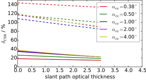
parti-cle shapes. The latter shows the relative uncertainties in CSR

δCSRfor the same parameters, computed as

δCSR=

CSRmax−CSRmin

0.5·(CSRmax+CSRmin)

.

In both graphs solid lines stand for a fixedreff of 25 µm

and dashed lines for an undefined effective radius. Again it

0.0 0.5 1.0 1.5 2.0 2.5 3.0 3.5 4.0 4.5

slant path optical thickness

0

20

40

60

80

100

120

140

δ

/

%

α

=

0.38

α

=

0.50

α

=

1.00

α

=

2.00

α

=

4.00

Fig. 4. Relative uncertaintyδCSRfor certain fields of view (legend

gives opening half-angle in degrees). Solid lines: forreff=25 µm

and undefined ice particle shape. Dashed lines: for undefinedreff

and ice particle shape.

becomes apparent that knowledge about the effective radius considerably reduces the uncertainties.

3 Results

So far the components of our method have been treated in-dividually. In this section we apply the complete circumsolar retrieval chain on real data; that is, we process the SEVIRI measurements identified to contain cirrus clouds by COCS through the APICS cloud property retrieval. The obtainedreff

values are used to pick appropriate values from thek LUT. These together with the optical thickness from APICS are then used in Eq. (14) to calculate CSR.

We compare CSR retrieval results for different ice particle shape assumptions. Maps of the average circumsolar irradi-ance for the two Baum ice particle parameterizations are pre-sented and, finally, a validation against ground measurements of the CSR is offered.

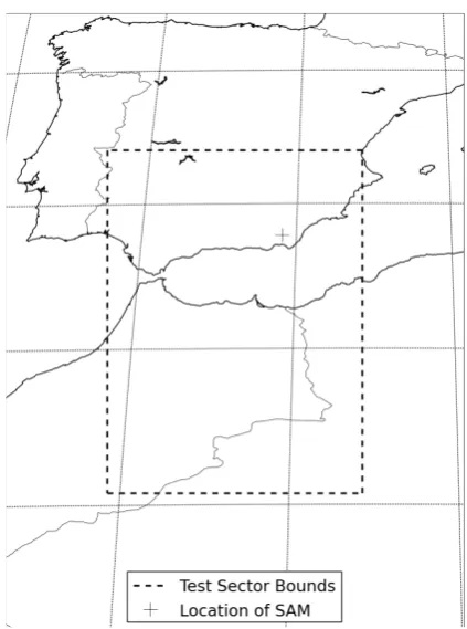
A test sector of 189×252 satellite pixels within the whole MSG disk of 3712×3712 pixels was selected for evaluation. The sector includes the southern part of the Iberian Peninsula as well as parts of northern Africa (see Fig. 5). One year of data was evaluated for this sector (May 2011–April 2012). Unless stated otherwise, MSG-related statements refer to this area. Ocean pixels and pixels containing continental water surfaces were excluded using a land–water mask from the EUMETSAT Land Surface Analysis Satellite Applications Facility.

3.1 Consideration of different ice particle shapes in the whole retrieval chain

B. Reinhardt et al.: Determination of circumsolar radiation from Meteosat Second Generation 831

Fig. 3.Uncertainty in circumsolar irradiance for certain fields of

view (legend gives opening half angle in degrees). Solid lines: for

reff= 25µmand undefined ice particle shape. Dashed lines: for

un-definedreffand ice particle shape.

Fig. 4.Relative uncertaintyδCSRfor certain fields of view (legend

gives opening half angle in degrees). Solid lines: forreff= 25µm

and undefined ice particle shape. Dashed lines: for undefinedreff

and ice particle shape.

Fig. 5.Map covering the test sector. SEVIRI pixels are evaluated

inside the sector (only over land). The cross marks the location of the SAM instrument at the Plataforma Solar de Almer´ıa (Sect. 3.3).

2

4

6

8

10

droxtal

rosette 6

rough aggregate

hollow column

solid column

Baum 3.5

Baum 2.0

0.0

0.2

0.4

0.6

0.8

1.0

CSR(

α

=2

.

5

)

0.0

0.1

0.2

0.3

0.4

0.5

0.6

Relative occurrence / %

Fig. 6.Histograms of the relative occurrence of circumsolar ratio

(CSR) values under the conditionItot,α=2.5>200 W m−2with

re-spect to the total number of SEVIRI measurements withItot,α=2.5> 200 W m−2

for one year within the test sector considering the dif-ferent ice particle shapes.

Fig. 5. Map covering the test sector. SEVIRI pixels are evaluated

inside the sector (only over land). The cross marks the location of the SAM instrument at the Plataforma Solar de Almería (Sect. 3.3).

Therefore the overall variability was investigated by apply-ing the complete retrieval chain yieldapply-ing circumsolar radia-tion from SEVIRI measurements several times using differ-ent setups.

To this end CSR values for a limiting angleα=2.5◦have been retrieved from 1 yr within the SEVIRI test sector. This was done for the five ice particle shapes and the two shape mixtures described in Sect. 2.3; that is, seven distinct APICS runs were performed with different cloud optical properties. In the following conversion from the retrieved cloud proper-ties to CSR values, optical properproper-ties for the same particle shape were used as in the corresponding APICS run. There-fore seven different CSR data sets were obtained in total.

A histogram of the occurrence of CSR values was com-puted for every ice particle shape considering the whole do-main, excluding, however, measurements for which total ir-radiance valuesItot,α=2.5◦≤200 W m−2were calculated. We consideredItot,α=2.5◦=200 W m−2 _{to be the lower}

opera-tion limit of a hypothetical CST plant. These histograms are shown in Fig. 6, which gives a first illustration of the un-certainty induced by not knowing the particle shape. The Baum optical properties are based on a realistic mixture of particle shapes, and thus an operational retrieval would rely on them rather than on individual particle shapes. There-fore the corresponding lines are highlighted. The occurrence

2

4

6

8

10

droxtal

rosette 6

rough aggregate

hollow column

solid column

Baum 3.5

Baum 2.0

0.0

0.2

0.4

0.6

0.8

1.0

CSR(

α

=2

.

5

)

0.0

0.1

0.2

0.3

0.4

0.5

0.6

Relative occurrence / %

Fig. 6. Histograms of the relative occurrence of circumsolar

ra-tio (CSR) values under the condira-tion Itot,α=2.5>200 W m−2

with respect to the total number of SEVIRI measurements with

Itot,α=2.5>200 W m−2for 1 yr within the test sector considering

the different ice particle shapes.

is shown relative to the number of all measurements that fulfil Itot,α=2.5◦>200 W m−2, i.e. inclusive corresponding clear-sky measurements. For the calculation ofItot,α=2.5◦the clear-sky direct irradianceI0is required (Eq. 12). It was

ob-tained from libRadtran calculations assuming an elevation of 0 m a.s.l. everywhere. In the presence of water clouds,

Itot,α=2.5◦ was assumed to be below the 200 W m−2 thresh-old because water clouds are at most times too optically thick to allow higher values. These cases were identified with a general cloud mask from EUMETSAT (EUM OPS DOC 09 5164; EUM MET REP 07 0132). Pixels marked cloudy in this mask but not in the COCS cirrus cloud mask were assumed to contain water clouds. While on average 22 % of the SEVIRI measurements in the test data set produce a cirrus cloud detection, only 8–10 % additionally satisfy the 200 W m−2criterion (depending on the assumed ice particle shape).

To gain insight into how much the retrieval results scatter, Fig. 7 shows, as an example, the distribution of CSR from the retrieval with Baum v2.0 applied to a subset of SEVIRI measurements – namely to the subset for which the retrieval with Baum v3.5 yielded CSR values between 0.17 and 0.18. Ideally, if the ice particle shape had no influence, all Baum v2.0 results would also fall into the same interval. However in reality the distribution is clearly wider.

832 B. Reinhardt et al.: Determination of circumsolar radiation from Meteosat Second Generation

Fig. 7. Normalized distribution of retrieval results using “Baum

v2.0” for SEVIRI measurements for which the retrieval with “Baum v3.5” yielded circumsolar ratio (CSR) values between 0.17 an 0.18. Dashed lines mark the 25th and 75th percentiles (q25andq75).

Fig. 7. Normalized distribution of retrieval results using Baum

v2.0 for SEVIRI measurements for which the retrieval with Baum v3.5 yielded circumsolar ratio (CSR) values between 0.17 an 0.18. Dashed lines mark the 25th and 75th percentiles (q25andq75).

(specified in they axis label of each panel). The resulting new CSR distribution is colour-coded along they axis. Fig-ure 7 shows the Baum v2.0 CSR distribution within one of these subsets and is simply a vertical cross section through the upper left panel. From Fig. 8 one can see that hollow-columns and rough aggregates have rather narrow distribu-tions but also show some curvature – implying a bias com-pared to Baum v3.5. Rosettes, which account for a good share of the particles with a maximum dimension larger than 150 µm in Baum v3.5, produce a relatively narrow distribu-tion close to the 1:1 line. Droxtals, which are only used to represent small particles in the two Baum parameterizations, yield quite different CSR results compared to Baum v3.5: the results within the individual CSR subsets scatter widely and most times droxtals yield smaller CSR values than Baum v3.5 (distribution is curved to lower values). The distribu-tions for Baum v2.0 and solid columns are quite similar, be-ing rather broad with no clear bias visible.

3.2 Circumsolar irradiance

The average circumsolar irradiance during CST plant op-eration is strongly dependent on the lower DNI limit the plant can work at. Nevertheless, we calculated the mean cir-cumsolar irradiance in W m−2 _{for a FOV of α=2.5}◦ _to

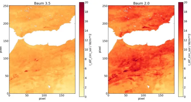
provide an example. Again we considered only values for this for which the total irradianceItot,α=2.5◦ was computed as being above 200 W m−2. Figure 9 shows two maps of the circumsolar irradiance averaged over all time steps with

Itot,α=2.5◦>200 W m−2 – one for the Baum v3.5 optical properties and one for Baum v2.0. The values for Baum v2.0 are on average about 50 % higher than for Baum v3.5 but the

regional distribution patterns are similar. Therefore intra-site comparisons are possible with our method with considerably less dependence on the assumed ice particle shape. There are few red pixels visible in the figure that stand out from their environment. These are caused by unusually frequent cloud detections by COCS at these locations. In this example the Baum parameterizations also mark the extremes of the tem-porally and spatially averaged values and the HEY param-eterizations lie in between (not shown here). Interestingly, HEY aggregates produce the mean circumsolar irradiance value closest to Baum v3.5 result and HEY solid columns show the mean value closest to Baum v2.0. Aggregates are the only roughened particles of the HEY data set which may explain the similarity of their results to the ones obtained with Baum v3.5. Considering the similarities between HEY solid columns and Baum v2.0 it should be mentioned that the medium-sized particles in Baum v2.0 are mainly represented by solid columns. Similarities between Baum v3.5 and HEY aggregates as well as between Baum v2.0 and HEY solid columns are also visible in the histograms of Fig. 6.

3.3 Validation with ground measurements

In this section we compare our results with ground mea-surements of the CSR performed at the Plataforma Solar de Almería (location marked in Fig. 5) with the system pre-sented in (Wilbert et al., 2013). This system consists of the Sun and Aureole Measurement system (SAM) (DeVore et al., 2009), a Cimel sun photometer that is part of AERONET (Holben et al., 1998) and dedicated post-processing software. The software determines the broadband sunshape and the broadband circumsolar ratio based on the spectral radiance measurements from the SAM and the AERONET data. This involves also the use of a slightly modified version of the SMARTS2.9.5 code (Gueymard, 2001). CSR measurements were available for the same period of 1 yr length that was evaluated in the previous sections (May 2011–April 2012). The SAM-based measurements show varying frequency but were generally done at least once per minute, except for a few days which had to be discarded due to technical failures of the instrument.

Fig. 8. Normalized circumsolar ratio (CSR) retrieval distributions for 100 bins of CSR from Baum v3.5 (xaxis, bin width 0.01). Dashed lines markq25andq75; that is, they enclose 50 % of the measurements. Black vertical line in upper left panel marks the cross section that is

displayed in Fig. 7.

The retrieval results from three consecutive SEVIRI mea-surements at timest0−15 min,t0andt0+15 min were

aver-aged to reduce short-term variability, which can deteriorate the validation results if the SEVIRI and SAM measurements are not perfectly collocated.

SAM only measures CSR at one place, while our method delivers an average CSR for several square kilometres. To alleviate this scale discrepancy we brought the ground mea-surements to the same time grid as the SEVIRI measure-ments by averaging them within a symmetrical time span1t

aroundt0. The averaging of the CSR from SAM was done

ap-plying a Gaussian weighting functionwto the measurements

w=exp

_−2(t−t

0)2

1t2

, (17)

witht being the time of the SAM measurement andt0

be-ing the time of the central SEVIRI measurement. Underlybe-ing this is the assumption that a temporal average of the advected cloud properties is more representative of the spatial average of cloud properties that we retrieve at distinct times from SE-VIRI. We found the averaging time of1t=35 min to deliver good agreement between satellite and ground measurements, and did not see much better agreement for longer averaging times. Only SAM measurements meeting the condition

|t−t0|< 1t (18)

Fig. 9.Circumsolar irradiance for a limiting angle of 2.5◦averaged over all time steps in the test dataset withItot,α=2.5◦>200 W m−2.

0.0 0.1 0.2 0.3 0.4 0.5 0.6 0.7

CSR SAM

0.0

0.1

0.2

0.3

0.4

0.5

0.6

0.7

CSR APICS Baum 3.5

All data

Manually filtered

0.0 0.1 0.2 0.3 0.4 0.5 0.6 0.7

CSR SAM

0.0

0.1

0.2

0.3

0.4

0.5

0.6

0.7

CSR APICS Baum 2.0

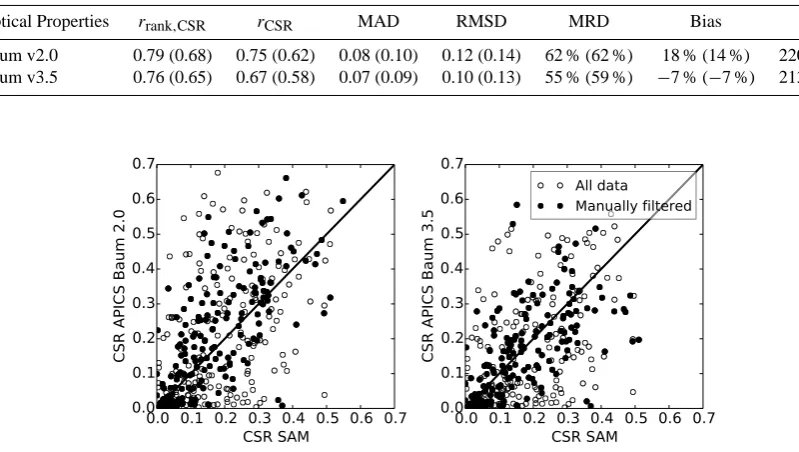
Fig. 10.Scatter plots for the shortened validation time series (May 2011–Jun. 2011). Left panel: CSR retrieved using “Baum v2.0”. Right

panel: CSR retrieved using “Baum v3.5”. Filled circles indicate that the data pair has passed the manual cumulus cloud screening on the basis of all-sky images.

04:00:0006:00:0008:00:0010:00:0012:00:0014:00:0016:00:0018:00:0020:00:0022:00:00 0.0

0.1 0.2 0.3 0.4 0.5 0.6 0.7

CSR

2011-05-11

SAM

APICS Baum 2.0

04:00:0006:00:0008:00:0010:00:0012:00:0014:00:0016:00:0018:00:0020:00:0022:00:00

2011-06-05

04:00:0006:00:0008:00:0010:00:0012:00:0014:00:0016:00:0018:00:0020:00:0022:00:00

2011-06-11

Fig. 11.Exemplary excerpt of the circumsolar ratio (CSR) time series used for the validation. In total 107 data pairs are shown. Grey symbols

indicate that water clouds were identified in the manual screening of sky camera images. Time is given as UTC.

Fig. 9. Circumsolar irradiance for a limiting angle of 2.5◦averaged over all time steps in the test data set withItot,α=2.5◦>200 W m−2.

Before comparing CSR values for a 2.5◦ FOV the mea-surements were filtered: only time steps with a positive cir-rus cloud detection from MSG were considered. Furthermore we required the total irradianceItot,α=2.5◦calculated from the averaged SEVIRI measurements to be above 200 W m−2as in Sect. 3.2 to ensure relevance for CST plants.

The following validation measures were calculated using the N remaining CSR pairs in the time series: the relative bias, the mean absolute deviation (MAD), the root-mean-square deviation (RMSD), the median relative deviation (MRD), the Pearson correlationr(Wilks, 2005, Eq. 3.23) and the Spearman rank correlationrrank(Wilks, 2005, Eq. 3.28).

We show the RMSD and the Pearson correlation since they are widely used validation measures; however it should be noted that they have to be interpreted with care because the deviations between SAM and the satellite retrieved values are not normally distributed and we do not expect a truly lin-ear relationship between the CSR from SAM and from our method. This is because errors in1korτswill not propagate

linearly (comp. Eq. 15). The Spearman rank correlationrrank

is simply the Pearson correlation applied not on the data, but on the ranks of the data. It is not a measure of linear relation-ship but of monotone relationrelation-ship. The Pearson correlation is neither robust nor resistant, whereas the Spearman rank correlation is – it requires no assumption about the kind of monotone relationship (e.g. linear) and is not unduly influ-enced by a few outliers (Wilks, 2005, Chap. 3).

Bias= PN

i=1CSRSEVIRI,i−PNi=1CSRSAM,i PN

i=1CSRSAM,i

(19)

MAD=

N X

i=1

CSRSEVIRI,i−CSRSAM,i

N (20)

RMSD= v u u t

N X

i=1

(CSRSEVIRI,i−CSRSAM,i)2

N (21)

MRD=q50

_CSR

SEVIRI,i−CSRSAM,i CSRSAM,i

(22)

In Table 2 the different validation measures are listed. The rank correlation of 0.48 and 0.54 and the MAD values of 0.11 show that there are considerable differences between the time series if we look at instantaneous values. This is also confirmed by the MRD of 75 and 74 % meaning that 50 % of the derived CSR values deviate by more than 75 or 74 % from the SAM measurements. It should be noted, however, that the largest relative deviations occur for very small values of the CSR, which are irrelevant in practice.

Table 2. Results of the comparison of CSR measured from ground and retrieved from SEVIRI for different setups: rank correlationrrank,CSR,

Pearson correlationrCSR, mean absolute deviation MAD, root-mean-square deviation RMSD, median relative deviation MRD, bias and the

number of compared data pairsN.

Optical Properties rrank,CSR rCSR MAD RMSD MRD Bias N

Baum v2.0 0.54 0.50 0.11 0.16 75 % 4 % 2021 Baum v3.5 0.48 0.44 0.11 0.15 74 % −11 % 1890

Table 3. Same as Table 2 but for the shortened time series (1 May 2011–30 June 2011) which was manually cumulus-screened. Values in

parenthesis are for unscreened time series.

Optical Properties rrank,CSR rCSR MAD RMSD MRD Bias N

Baum v2.0 0.79 (0.68) 0.75 (0.62) 0.08 (0.10) 0.12 (0.14) 62 % (62 %) 18 % (14 %) 220 (407) Baum v3.5 0.76 (0.65) 0.67 (0.58) 0.07 (0.09) 0.10 (0.13) 55 % (59 %) −7 % (−7 %) 213 (386)

18 B. Reinhardt et al.: Determination of circumsolar radiation from Meteosat Second Generation

Fig. 9.Circumsolar irradiance for a limiting angle of 2.5◦averaged over all time steps in the test dataset withItot,α=2.5◦>200 W m−2

.

0.0 0.1 0.2 0.3 0.4 0.5 0.6 0.7

CSR SAM

0.0

0.1

0.2

0.3

0.4

0.5

0.6

0.7

CSR APICS Baum 3.5

All data

Manually filtered

0.0 0.1 0.2 0.3 0.4 0.5 0.6 0.7

CSR SAM

0.0

0.1

0.2

0.3

0.4

0.5

0.6

0.7

CSR APICS Baum 2.0

Fig. 10.Scatter plots for the shortened validation time series (May 2011–Jun. 2011). Left panel: CSR retrieved using “Baum v2.0”. Right panel: CSR retrieved using “Baum v3.5”. Filled circles indicate that the data pair has passed the manual cumulus cloud screening on the basis of all-sky images.

04:00:0006:00:0008:00:0010:00:0012:00:0014:00:0016:00:0018:00:0020:00:0022:00:00

0.0 0.1 0.2 0.3 0.4 0.5 0.6 0.7

CSR

2011-05-11 SAM

APICS Baum 2.0

04:00:0006:00:0008:00:0010:00:0012:00:0014:00:0016:00:0018:00:0020:00:0022:00:00

2011-06-05

04:00:0006:00:0008:00:0010:00:0012:00:0014:00:0016:00:0018:00:0020:00:0022:00:00

2011-06-11

Fig. 11.Exemplary excerpt of the circumsolar ratio (CSR) time series used for the validation. In total 107 data pairs are shown. Grey symbols indicate that water clouds were identified in the manual screening of sky camera images. Time is given as UTC.

Fig. 10. Scatter plots for the shortened validation time series (May 2011–June 2011). Left panel: CSR retrieved using Baum v2.0. Right

panel: CSR retrieved using Baum v3.5. Filled circles indicate that the data pair has passed the manual cumulus cloud screening on the basis of all-sky images.

values decrease. For Baum v3.5 the bias stays unchanged, while for Baum v2.0 a slight increase in the bias is observed. The MRD, which features a certain robustness in regard to outliers, improves only slightly from Baum v3.5 and stays unchanged for Baum v2.0.

Figure 10 contains scatter plots for the shortened evalu-ation time series for Baum v2.0 and Baum v3.5. Displayed are all data from 1 May 2011 to 30 June 2011. Filled circles mark data pairs which passed the manual cumulus screen-ing. The figure confirms the information from the numeri-cal validation measures: the cumulus screening reduces the scatter. A cloud detection excluding cumulus-contaminated pixels would thus be desirable for future applications.

Excerpts of the evaluated time series are shown in Fig. 11. We selected those three days that contain the most data pairs from shortened data series (May–June 2011). From the figure it becomes apparent that the temporal evolution of the CSR measured by SAM is in general captured by the satellite time

series but due to timing and amplitude errors the CSR values at a given time often disagree. This results in the scatter seen in Fig. 10.

836 B. Reinhardt et al.: Determination of circumsolar radiation from Meteosat Second Generation

Fig. 9.Circumsolar irradiance for a limiting angle of 2.5◦averaged over all time steps in the test dataset withItot,α=2.5◦>200 W m−2.

0.0 0.1 0.2 0.3 0.4 0.5 0.6 0.7

CSR SAM

0.0

0.1

0.2

0.3

0.4

0.5

0.6

0.7

CSR APICS Baum 3.5

All data

Manually filtered

0.0 0.1 0.2 0.3 0.4 0.5 0.6 0.7

CSR SAM

0.0

0.1

0.2

0.3

0.4

0.5

0.6

0.7

CSR APICS Baum 2.0

Fig. 10.Scatter plots for the shortened validation time series (May 2011–Jun. 2011). Left panel: CSR retrieved using “Baum v2.0”. Right

panel: CSR retrieved using “Baum v3.5”. Filled circles indicate that the data pair has passed the manual cumulus cloud screening on the basis of all-sky images.

04:00:00

06:00:00

08:00:00

10:00:00

12:00:00

14:00:00

16:00:00

18:00:00

20:00:00

22:00:00

0.0

0.1

0.2

0.3

0.4

0.5

0.6

0.7

CSR

2011-05-11

SAM

APICS Baum 2.0

04:00:00

06:00:00

08:00:00

10:00:00

12:00:00

14:00:00

16:00:00

18:00:00

20:00:00

22:00:00

2011-06-05

04:00:00

06:00:00

08:00:00

10:00:00

12:00:00

14:00:00

16:00:00

18:00:00

20:00:00

22:00:00

2011-06-11

Fig. 11.Exemplary excerpt of the circumsolar ratio (CSR) time series used for the validation. In total 107 data pairs are shown. Grey symbols

indicate that water clouds were identified in the manual screening of sky camera images. Time is given as UTC.

Fig. 11. Exemplary excerpt of the circumsolar ratio (CSR) time series used for the validation. In total 107 data pairs are shown. Grey symbols

indicate that water clouds were identified in the manual screening of sky camera images. Time is given as UTC.

B. Reinhardt et al.: Determination of circumsolar radiation from Meteosat Second Generation 19

0.0 0.1 0.2 0.3 0.4 0.5 0.6 0.7 0.8

CSR(

α

=2

.

5

)

0

100

200

300

400

500

600

700

#

N = 2021

APICS Baum 2.0

SAM Measurement

0.0 0.1 0.2 0.3 0.4 0.5 0.6 0.7 0.8

CSR(

α

=2

.

5

)

N = 1890

APICS Baum 3.5

SAM Measurement

Fig. 12.Histograms of the circumsolar ratio (CSR) time series measured by SAM and retrieved from SEVIRI that were used for the validation in Sect. 3.3.

Fig. 12. Histograms of the circumsolar ratio (CSR) time series measured by SAM and retrieved from SEVIRI that were used for the validation

in Sect. 3.3.

4 Summary and conclusions

A method to determine circumsolar radiation from measure-ments of the geostationary satellites of the Meteosat Second Generation family was developed. To achieve this, several components were linked together and improved where nec-essary. The Monte Carlo radiative transfer model MYSTIC was extended by introducing a sun disk instead of a point source such that it can simulate the circumsolar region with high accuracy. With this tool at hand, it was possible to estab-lish a database of coefficients that enables the computation of circumsolar radiation by simple analytical expressions from cloud properties instead of performing time-consuming ra-diative transfer simulations. This was facilitated by the de-velopment of a theoretical basis that avoids a dependence on optical thickness in the database. To obtain CSR values from satellite measurements, the database is used in conjunc-tion with the cloud property retrieval from the APICS frame-work. APICS was improved by creating an albedo data set that is consistent with the cloud property retrieval algorithm and that optimizes the retrieval’s success rate. Furthermore APICS was extended with new look-up tables for individual

ice particle shapes and the Baum v3.5 ice particle mixture to allow for an uncertainty analysis.

Retrievals of circumsolar radiation show that the uncer-tainties in the complete retrieval chain due to assumptions of the ice particle shape can sum up to 50 %. A validation of re-trieved CSR values with SAM-based measurements shows that considerable errors must be expected if instantaneous values are compared: the mean absolute deviation is 0.11 and the median relative deviation is approximately 75 %. Nev-ertheless, the frequency distribution of the satellite derived CSR is in good agreement with the ground measurements if the two Baum optical properties are used. In general Baum v2.0 produces slightly higher CSR values than Baum v3.5, which is also reflected in the bias values of 4 % and−11 %, respectively, compared to the ground measurements. A man-ual data screening indicates that the presence of sub-scale water clouds below the cirrus compromises the results. A de-tection and appropriate treatment of “mixed cloud” pixels is an open point for further development.

measurements it is cheap. Satellite data are also readily avail-able for many regions of the world for longer time spans than any of the time series of ground measurements available so far. Furthermore the method allows for easy comparison of the circumsolar radiation characteristics of several sites as long as they are within the field of view of the same satellite. The further development of satellite-based cloud property re-trievals can improve the circumsolar radiation products since the errors in the retrieved cloud properties are a main source of uncertainty in circumsolar radiation. In particular, further information about the ice particle shape composition would help to further reduce the uncertainty.

The presented parameterization with its efficient look-up table approach can in principle be extended and applied to other data sources as well. Aerosols, the other significant source for CST-relevant circumsolar radiation besides cirrus clouds, could be treated by combining the parameterization with an aerosol-resolving weather forecast model.

Supplementary material related to this article is available online at http://www.atmos-meas-tech.net/7/ 823/2014/amt-7-823-2014-supplement.zip.

Acknowledgements. Special thanks go to Stephan Kox (DLR) for

the provision of COCS data. We also thank the AERONET and RIMA staff for their support. The calibration of the Cimel sun photometer was performed at AERONET-EUROPE, supported by ACTRIS (EU FP7 2007–2013). We also thank Christian Guey-mard for providing the SMARTS software that was used in the processing of the ground data and his support for the development of the ground-based measurement system. This study was partially founded by the EU’s FP7 through the project “Solar Facilities for the European Research Area – SFERA”. We also would like to thank Silke Groß and Gerard Kilroy, who provided helpful comments on the manuscript.

The service charges for this open access publication have been covered by a Research Centre of the Helmholtz Association.

Edited by: S. Schmidt

References

Baum, B., Heymsfield, A., Yang, P., and Bedka, S.: Bulk scattering models for the remote sensing of ice clouds, Part 1: Microphysi-cal data and models, J. Appl. Meteorol., 44, 1885–1895, 2005a. Baum, B., Yang, P., Heymsfield, A., Platnick, S., King, M. D.,

Hu, Y. X., and Bedka, S.: Bulk scattering models for the remote sensing of ice clouds, Part 2: Narrowband models, J. Appl. Me-teorol., 44, 1896–1911, 2005b.

Baum, B. A., Yang, P., Heymsfield, A. J., Schmitt, C. G., Xie, Y., Bansemer, A., Hu, Y.-X., and Zhang, Z.: Improvements in short-wave bulk scattering and absorption models for the remote sens-ing of ice clouds, J. Appl. Meteorol. Climatol., 50, 1037–1056, doi:10.1175/2010JAMC2608.1, 2011.

Bugliaro, L., Zinner, T., Keil, C., Mayer, B., Hollmann, R., Reuter, M., and Thomas, W.: Validation of cloud property re-trievals with simulated satellite radiances: a case study for SE-VIRI, Atmos. Chem. Phys., 11, 5603–5624, doi:10.5194/acp-11-5603-2011, 2011.

Bugliaro, L., Mannstein, H., and Kox, S.: Ice cloud properties from space, in: Atmospheric Physics, edited by: Schumann, U., 417– 432, Springer-Verlag Berlin Heidelberg, 2012.

Bugliaro, L., Ostler, A., Wirth, M., Emde, C., and Schumann, U.: Validation of cirrus detection and cirrus optical thickness derived from MSG/SEVIRI with an airborne high spectral resolution li-dar, Atmos. Meas. Tech., in preparation, 2013.

Buie, D. and Monger, A.: The effect of circumsolar radiation on a solar concentrating system, Sol. Energy, 76, 181–185, 2004. Buie, D., Monger, A., and Dey, C.: Sunshape distributions

for terrestrial solar simulations, Sol. Energy, 74, 113–122, doi:10.1016/S0038-092X(03)00125-7, 2003.

Buras, R. and Mayer, B.: Efficient unbiased variance reduction tech-niques for monte carlo simulations of radiative transfer in cloudy atmospheres: the solution, J. Quant. Spectr. R. Transf., 112, 434– 447, doi:10.1016/j.jqsrt.2010.10.005, 2011.

CIMO Guide: Guide to Meteorological Instruments and Methods of Observation, 7th Edn., Tech. rep., World Meteorological Organi-zation, 681 pp., Chap. 7.2, 2008.

DeVore, J. G., Stair, A. T., LePage, A., Rall, D., Atkin-son, J., Villanucci, D., Rappaport, S. A., Joss, P. C., and Mc-Clatchey, R. A.: Retrieving properties of thin clouds from so-lar aureole measurements, J. Atmos. Ocean. Technol., 26, 2531– 2548, doi:10.1175/2009JTECHA1289.1, 2009.

EUM MET REP 07 0132: Cloud Detection for MSG – Algo-rithm Theoretical Basis Document, EUMETSAT, Darmstadt, Germany, v2 edn., EUM/MET/REP/07/0132, 2007.

EUM OPS DOC 09 5164: Cloud Mask Factsheet, EUMETSAT, Darmstadt, Germany, v1 edn., EUM/OPS/DOC/09/5164, 2010. EUM OPS DOC 09 5165: SEVIRI – clear sky reflectance

map factsheet, EUMETSAT, Darmstadt, Germany, v2b edn., EUM/OPS/DOC/09/5165, 2011.

Ewald, F., Bugliaro, L., Mannstein, H., and Mayer, B.: An im-proved cirrus detection algorithm MeCiDA2 for SEVIRI and its evaluation with MODIS, Atmos. Meas. Tech., 6, 309–322, doi:10.5194/amt-6-309-2013, 2013.

Fricke, C., Ehrlich, A., Wendisch, M., and Bohn, B.: Wiss. Mit-teil. Inst. f. Meteorol. Univ. Leipzig, vol. 50, chap. Infuence of Surface Albedo Inhomogeneities on Remote Sensing of Optical Thin Cirrus Cloud Mikrophysics, edited by: Raabe, A., Univer-sität Leipzig, 1–10, 2012.

Grassl, H.: Calculated circumsolar radiation as a function of aerosol type, field of view, wavelength, and optical depth, Appl. Optics, 10, 2542–2543, 1971.

Greuell, W. and Roebeling, R.: Towards a standard proce-dure for validation of satellite-derived cloud liquid wa-ter path, J. Appl. Meteorol. Climatol., 48, 1575–1590, doi:10.1175/2009JAMC2112.1, 2009.

Gueymard, C.: Parameterized transmittance model for direct beam and circumsolar spectral irradiance, Sol. Energy, 71, 325–346, 2001.

applica-tion to Meteosat-8/9 and MTSAT-1R, Atmos. Chem. Phys., 10, 11131–11149, doi:10.5194/acp-10-11131-2010, 2010.

Hansen, J. and Travis, L.: Light scattering in planetary atmospheres, Space Sci. Rev., 16, 527–610, doi:10.1007/BF00168069, 1974. Holben, B. N., Eck, T. F., Slutsker, I., Tanre, D., Buis, J. P.,

Set-zer, A., Vermote, E., Reagan, J. A., Kaufman, Y. J., Nakajima, T., Lavenu, F., Jankowiak, I., and Smirnov, A.: AERONET – a federated instrument network and data archive for aerosol char-acterization, Remote Sens. Environ., 66, 1–16, 1998.

Joseph, J. H., Wiscombe, W. J., and Weinman, J. A.: The Delta–Eddington approximation for radiative flux trans-fer, J. Atmos. Sci., 33, 2452–2459, doi:10.1175/1520-0469(1976)033<2452:TDEAFR>2.0.CO;2, 1976.

Kinne, S., Akermann, T., Shiobara, M., Uchiyama, A., Heyms-field, A., Miloshevich, L., Wendell, J., Eloranta, E., Purgold, C., and Bergstrom, R.: Cirrus cloud radiative and microphysical properties from ground observations and in situ measurements during FIRE 1991 and their application to exhibit problems in cirrus solar radiative transfer modeling, J. Atmos. Sci., 54, 2320– 2344, 1997.

Köpke, P., Reuder, J., and Schween, J.: Spectral variation of the solar radiation during an eclipse, Meteorol. Z., 10, 179–186, doi:10.1127/0941-2948/2001/0010-0179, 2001.

Kox, S.: Remote sensing of the diurnal cycle of optically thin cirrus clouds, Ph. D. thesis, Ludwig–Maximilians–Universität München, available at: http://nbn-resolving.de/urn:nbn:de:bvb: 19-151170, 2012.

Kox, S., Ostler, A., Vazquez-Navarro, M., Bugliaro, L., and Mannstein, H.: Optical properties of thin cirrus derived from the infrared channels of SEVIRI, in: EUMETSAT Meteorological Satellite Conference, Oslo, Norway, ISBN 978-92-9110-093-4, 2011.

Krebs, W., Mannstein, H., Bugliaro, L., and Mayer, B.: Technical note: a new day- and night-time Meteosat Second Generation Cirrus Detection Algorithm MeCiDA, Atmos. Chem. Phys., 7, 6145–6159, doi:10.5194/acp-7-6145-2007, 2007.

Mayer, B.: Radiative transfer in the cloudy atmosphere, Eur. Phys. J. Conferences, 1, 75–99, doi:10.1140/epjconf/e2009-00912-1, 2009.

Mayer, B. and Kylling, A.: Technical note: The libRadtran soft-ware package for radiative transfer calculations – description and examples of use, Atmos. Chem. Phys., 5, 1855–1877, doi:10.5194/acp-5-1855-2005, 2005.

McFarquhar, G. and Heymsfield, A.: The definition and significance of an effective radius for ice clouds, J. Atmos. Sci., 55, 2039– 2052, 1998.

Meirink, J. F., Roebeling, R. A., and Stammes, P.: Inter-calibration of polar imager solar channels using SEVIRI, Atmos. Meas. Tech., 6, 2495–2508, doi:10.5194/amt-6-2495-2013, 2013. Nakajima, T. and King, M. D.: Determination of the optical

thick-ness and effective particle radius of clouds from reflected solar radiation measurements, Part I: Theory, J. Atmos. Sci., 47, 1878– 1893, 1990.

Neumann, A. and Witzke, A.: The influence of sunshape on the DLR solar furnace beam, Sol. Energy, 66, 447–457, doi:10.1016/S0038-092X(99)00048-1, 1999.

Neumann, A., Witzke, A., Jones, S. A., and Schmitt, G.: Repre-sentative terrestrial solar brightness profiles, J. Sol. Energ.-T. ASME, 124, 198–204, doi:10.1115/1.1464880, 2002.

Noring, J., Grether, D., and Hunt, A.: Circumsolar radiation data: the Lawrence Berkely laboratory reduced data base, Tech. Rep. NREL/TP-262-44292, National Renewable Energy Laboratory, available at: http://rredc.nrel.gov/solar/pubs/circumsolar/index. html (last access: 16 March 2011), 1991.

Ostler, A.: Validierung von optischen Wolkeneigenschaften aus MSG-Daten, Mastert Tesis, Ludwig–Maximilians–Universität, München, 2011.

Rabl, A. and Bendt, P.: Effect of circumsolar radiation on perfor-mance of focusing collectors, J. Sol. Energy Eng., 104, 237, 1982.

Scheffler, H. and Elsässer, H.: Physik der Sterne und der Sonne, 2. Auflage, BI-Wiss.-Verl., 1990.

Schmetz, J., Pili, P., Tjemkes, S., Just, D., Kerkmann, J., Rota, S., and Ratier, A.: An introduction to Meteosat Second Generation (MSG), B. Am. Meteorol. Soc., 83, 977–992, 2002.

Schubnell, M.: Influence of circumsolar radiation on aperture, op-erating temperature and efficiency of a solar cavity receiver, Sol. Energ. Mat. Sol. C., 27, 233–242, doi:10.1016/0927-0248(92)90085-4, 1992.

Segal-Rosenheimer, M., Russell, P. B., Livingston, J. M., Ra-machandran, S., Redemann, J., and Baum, B. A.: Re-trieval of cirrus properties by sunphotometry: a new perspec-tive on an old issue, J. Geophys. Res.-Atmos., 118, 1–18, doi:10.1002/jgrd.50185, 2013.

Shiobara, M. and Asano, S.: Estimation of cirrus op-tical thickness from sun photometer measurements, J. Appl. Meteorol., 33, 672–681, doi:10.1175/1520-0450(1994)033<0672:EOCOTF>2.0.CO;2, 1994.

Strahler, A., Muller, J., and Members, M. S. T.: MODIS BRDF/Albedo product: algorithm theoretical basis document version 5.0, available at: http://modis.gsfc.nasa.gov/data/atbd/ atbd_mod09.pdf (last access: 22 March 2011), 1999.

Thomalla, E., Köpke, P., Müller, H., and Quenzel, H.: Circumsolar radiation calculated for various atmospheric conditions, Sol. En-ergy, 30, 575–587, doi:10.1016/0038-092X(83)90069-5, 1983. Wilbert, S., Reinhardt, B., DeVore, J., Röger, M., Pitz-Paal, R.,

and Gueymard, C.: Measurement of solar radiance profiles with the Sun and Aureole Measurement System (SAM), in: Proceed-ings of the SolarPACES Conference 20. – 23 September 2011, Granada, Spain, Publisher: SolarPACES, 2011.

Wilbert, S., Reinhardt, B., DeVore, J., Röger, M., Pitz-Paal, R., Gueymard, C., and Buras, R.: Measurement of solar radiance profiles with the Sun and Aureole Measurement System (SAM), J. Sol. Energ. Eng., 135, 041002, 2013.

Wilks, D.S.: Statistical Methods in the Atmospheric Sciences, Aca-demic Press Inc., 2nd Edn., 2005.

Winker, D. M., Vaughan, M. A., Omar, A., Hu, Y., Pow-ell, K. A., Liu, Z., Hunt, W. H., and Young, S. A.: Overview of the CALIPSO mission and CALIOP data process-ing algorithms, J. Atmos. Oceanic Technol., 26, 2310–2323, doi:10.1175/2009JTECHA1281.1, 2009.

Yang, P., Liou, K., Wyser, K., and Mitchell, D.: Parameterization of the scattering and absorption properties of individual ice crystals, J. Geophys. Res., 105, 4699–4718, 2000.