https://doi.org/10.5194/tc-11-2117-2017
© Author(s) 2017. This work is distributed under the Creative Commons Attribution 3.0 License.
Wave–ice interactions in the neXtSIM sea-ice model
Timothy D. Williams, Pierre Rampal, and Sylvain Bouillon
Nansen Environmental and Remote Sensing Center, Thormøhlensgate 47, N5006, Bergen, Norway and the Bjerknes Center for Climate Research, Bergen, Norway
Correspondence to:Timothy D. Williams ([email protected]) Received: 16 February 2017 – Discussion started: 28 February 2017
Revised: 1 August 2017 – Accepted: 7 August 2017 – Published: 7 September 2017
Abstract. In this paper we describe a waves-in-ice model (WIM), which calculates ice breakage and the wave radi-ation stress (WRS). This WIM is then coupled to the new sea-ice model neXtSIM, which is based on the elasto-brittle (EB) rheology. We highlight some numerical issues involved in the coupling and investigate the impact of the WRS, and of modifying the EB rheology to lower the stiffness of the ice in the area where the ice has broken up (the marginal ice zone or MIZ). In experiments in the absence of wind, we find that wind waves can produce noticeable movement of the ice edge in loose ice (concentration around 70 %) – up to 36 km, depending on the material parameters of the ice that are used and the dynamical model used for the broken ice. The ice edge position is unaffected by the WRS if the ini-tial concentration is higher (&0.9). Swell waves (monochro-matic waves with low frequency) do not affect the ice edge location (even for loose ice), as they are attenuated much less than the higher-frequency components of a wind wave spec-trum, and so consequently produce a much lower WRS (by about an order of magnitude at least).
In the presence of wind, we find that the wind stress dom-inates the WRS, which, while large near the ice edge, decays exponentially away from it. This is in contrast to the wind stress, which is applied over a much larger ice area. In this case (when wind is present) the dynamical model for the MIZ has more impact than the WRS, although that effect too is relatively modest. When the stiffness in the MIZ is lowered due to ice breakage, we find that on-ice winds produce more compression in the MIZ than in the pack, while off-ice winds can cause the MIZ to be separated from the pack ice.
1 Introduction
Wave–ice interactions have received a great deal of attention in recent years (e.g. Dumont et al., 2011; Kohout et al., 2014; Ardhuin et al., 2016, 2017), with progress in both modelling and measuring (particularly via synthetic aperture radar im-agery or SAR) waves in ice. To a large extent, this is due to climate change, with a series of record lows in both mini-mum and maximini-mum Arctic sea-ice extents in the last decade (e.g. Meier, 2017).
Specifically, large parts of the Arctic are becoming, and are expected to become, even more accessible for resource exploitation and shipping in the summer, whereas 10 years ago they were not (e.g. Stephenson et al., 2011). Associated with this low sea-ice extent is an increased open-water fetch available for wave generation, which means there are poten-tially more large-wave events in the Arctic in summer (e.g. in the Beaufort Sea in summer 2012; Thomson and Rogers, 2014). As well as being dangerous for shipping in them-selves, large waves also increase the amount of ice breakage in the marginal ice zone (MIZ), creating an extra hazard as small floes could potentially be thrown onto a ship deck, for example.
warm water to travel under the ice floes and enhance the melting from the edges. This was true even for large floes (∼1 km), when the lateral-to-horizontal surface-area ratio is quite small. Previously, this ratio was used to compute results which indicated lateral melting was unimportant for floes larger than∼100 m; Steele, 1992. Models for full numeri-cal FSDs (Zhang et al., 2016), where a histogram of floe-size bins can evolve in time as well as joint ice thickness and floe-size distributions, have been proposed (Horvat and Tziperman, 2015). In the latter model, each thickness cat-egory can have its own FSD. More parametric approaches have also been used (Dumont et al., 2011; Williams et al., 2013a; Bennetts et al., 2017).
On the sea-ice modelling side, there has been a lot of progress in making sea-ice dynamics more realistic, espe-cially in the Arctic pack. Rampal et al. (2016) presented a validation of the neXt-generation Sea Ice Model (neXtSIM), looking at sea-ice area and extent, sea-ice drift and the spa-tial scaling of sea-ice deformation derived from SAR (see also Bouillon and Rampal, 2015b). The dynamical core of neXtSIM is the EB sea-ice rheology, which is a thin elastic plate model with stresses constrained by a Mohr–Coulomb failure envelope. If stresses become too large and leave this envelope in a grid cell, the ice stiffness inside that cell is re-duced (in practice a parameter called “damage” is increased) in order to bring the stresses back onto the failure envelope (see Rampal et al., 2016, for more details). When one cell is highly damaged, the likelihood of the surrounding cells also becoming damaged is increased, leading to the rapid (i.e. af-ter a few sea-ice-model time steps) emergence of very lo-calised lines of damaged cells where sea ice can deform al-most freely. These lines of concentrated damage can accom-modate large deformation (i.e. opening, ridging and shear-ing) in a way that is similar to the so-called linear kinematic features that are observed from satellites (Kwok, 2001).
In this paper we demonstrate the coupling of a waves-in-ice model (WIM) to neXtSIM in an idealised domain. The physical effects included in the coupling are the break-up of ice by waves, the wave radiation stress (WRS) and an ad-ditional (optional) feedback to the sea-ice model where the ice stiffness is reduced where the ice is broken (in the MIZ). We conduct experiments with waves by themselves to see the impact of the WRS on the ice edge location and also with wind to see the relative importance of the wind stress and the WRS. In addition, we carry out some simulations to see the particular effects of the rheological change.
We also highlight some general numerical issues involved with coupling wave models and sea-ice models on different grids. In addition, we carry out some theoretical reformula-tions of the WIM to put the ice break-up model in the con-text of Mohr–Coulomb failure and test the sensitivity of the MIZ width to the Young’s modulus in particular, as well as the small-scale “cohesion” parameter in the WIM-breaking model. Its response to the Young’s modulus was previously uninvestigated.
2 Sea-ice model 2.1 Evolution equations
The ice is modelled as a thin elastic plate (e.g. Fung, 1965, Sect. 16.8) with a constitutive relation:
σ=C(Y∗, ν)ε, (1)
or in full
σ11 σ22 σ12
= Y∗
1−ν2
1 ν 0
ν 1 0
0 0 (1−ν)/2
ε11 ε22
2ε12
, (2)
whereσij andεij (i, j=1,2) are respectively the stress and
strain tensors, ν is Poisson’s ratio and Y∗ is the effective
Young’s modulus (depending on the concentrationcand the damaged), given by
Y∗(c, d)=Y0(1−d)e−C(1−c), (3)
whereCis the compactness parameter, andY0is the Young’s
modulus of fully compacted, undamaged ice.
The momentum balance equation we will use is the fol-lowing:
ρih
Du
Dt = ∇ ·(σh)− ∇P+τa+τo+τw,i. (4) Hereρi,h anduare the density, actual thickness, velocity
and internal stress tensor of the ice,∇ =(∂x, ∂y)Tis the
hor-izontal gradient, andτoandτa are the applied stresses by
the ocean and the atmosphere. These latter stresses come from quadratic drag laws. Note that we neglect the Corio-lis force and the gravitational force due to the slope of the ocean surface because of our idealised domain. Also appear-ing in Eq. (4) are the WRS,τw,iand the term involvingP,
which is a strictly positive pressure that provides resistance to compaction and ridging (i.e. it is only activated when the divergence∇ ·u<0):
P =max (
0,−P∗h
2e−C(1−c)∇ ·u |∇ ·u| + ˙εmin
)
, (5)
where P∗ is the pressure parameter, and ε˙min= (0.01/86 400)s−1 is the minimum divergence rate. If the ice becomes very damaged and loses its stiffness, this term prevents the ice from piling up and becoming too thick. As a default, we use the standard value of P∗=12 kPa,
We also have equations for the evolution of any conserved quantityφ:
Dφ
Dt = −φ (∇ ·u)+Sφ. (6)
φ could be concentration (c, also requiring c≤1), volume (ch) or variables relating to the damage (retrieved from(1−
d)−1). The termsSφ are thermodynamic source/sink terms
which are switched off for this paper, since the simulations are in an idealised setting and run for short durations. In an Eulerian frame of reference,
Dφ Dt =
∂φ
∂t +u· ∇φ, (7)
but since we work in a Lagrangian frame the relationship is simply Dφ/Dt=dφ/dt. The−φ (∇ ·u)term represents the conserved quantity decreasing if the divergence is positive e.g. if a triangle in the finite element mesh increased in area thenφshould drop in that triangle.
Like Williams et al. (2013a), we will parameterise the floe-size distribution in terms of the maximum floe size, Dmax(see Sect. 3.3), which we wish to advect like a tracer:
D(Dmax)/Dt=0.In the Lagrangian framework, advection is
usually exact, unless a local remeshing is required. This hap-pens if the triangles of the mesh become too deformed and requires (local) interpolation of the advected variable. De-tails on the remeshing procedure in the neXtSIM model can be found in Rampal et al. (2016). Additional (global) inter-polation is required to obtain Dmaxon the fixed grid of the
WIM (see Sect. 4). We found that transporting and interpo-latingDmaxitself led to some errors, which were reduced by
transporting an auxiliary variableNfloes=c/Dmax2 according
to D
Dt log(Nfloes)
= D
Dt log(c)
, (8)
or to progress from the neXtSIM time stepnton+1.Nfloes
should change according toNfloes(n+1)=c(n+1)Nfloes(n) /c(n)and be interpolated when either regridding or communication with the WIM is required.
The evolution of stress and damage from time step nto n+1 is done via an intermediate stress calculation:
σ0=σ(n)+C(c, d)ε˙1t, (9a)
σ(n+1)=9σ0, (9b) d(n+1)=1−9(1−d(n))+8d1t, (9c)
where8d is a thermodynamic source term (again not used
here), while9 (0< 9≤1) is a factor determined from the position of the stress vector relative to the Mohr–Coulomb failure envelope, described in Sect. 2.3. There is no continu-ous version of Eq. (9), since fracturing is an extremely rapid process, well below our typical time step1t.
2.2 Uncoupled neXtSIM simulation
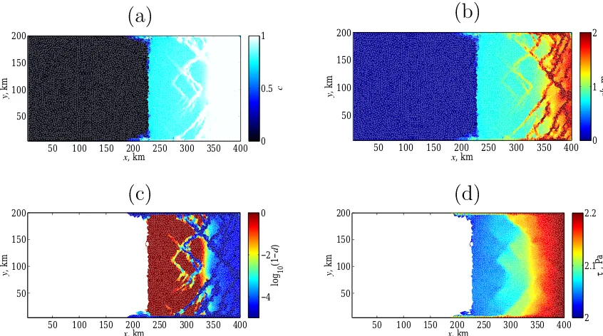
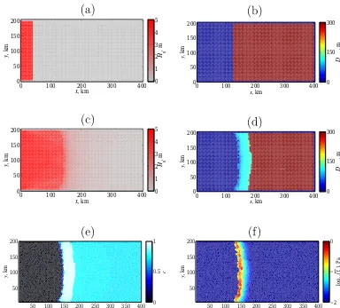
Since the damage variabled is probably unfamiliar to most readers, here we include an example simulation illustrating its main role in the EB rheology. Figure 1 shows four fields after a 2-day simulation. The wind stress plotted is calculated from the quadratic drag law
τa=ρaCd,a|ua−u|(ua−u), (10)
where ρa=1.3 kg m−3 and ua are the density and 10
m-velocity of the air, whileCd,a=7.6×10⁻³is the drag
coef-ficient of the wind on the ice. The gradient in the wind stress comes from the differences in relative velocity. We have plot-ted this stress as a reference for when we discuss the WRS.
Initially, the concentration was relatively low, so the inter-nal stress was also low (see the formulae forY∗ andP in
Eqs. 3, 5), meaning the ice was almost in free drift, being compressed against the right-hand boundary. As the concen-tration increased, the internal stress increased, causing it to fail (increase d) in localised regions. Comparing the dam-age with the concentration and thickness, it can be seen that the regions of high compression and thickening correspond to the regions where the damage is highest. This is the usual role (without waves) of the damage – to produce localised de-formation and features such as thicker regions (under shear-ing or convergent conditions, such as in the current simula-tion) and leads (under shearing or divergent conditions). We note here that the initial combination ofc=0.7 (loose ice) with no damage is not inconsistent since the damage only in-creases if the concentration is high, although the reasons for it usually being initialised to zero are (i) for simplicity and (ii) since it is not an observable variable. It then evolves with the other variables in response to the applied forcings. 2.3 Mohr–Coulomb failure
Letσ1 andσ2be the principal stresses, with compressions
corresponding to positive stresses. Then a stress state is within the Mohr–Coulomb failure envelope if the conditions σ2≤σc+qσ1, σ1≤σc+qσ2, (11a) σN,min≤σN≡
1
2(σ1+σ2)≤σN,max, (11b) are satisfied (Schulson et al., 2006; Dansereau et al., 2016; Rampal et al., 2016), where
σc=
2τ0 p
µ2+1−µ, q= q
µ2+1+µ2 ,
σN,min= −
5σc
6(q−1), σN,max= 75
4 τ0,
andτ0is the cohesion, andµis the internal friction
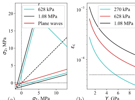
coeffi-cient. See Fig. 2a for some example envelopes (τ0=629 and
50 100 150 200 250 300 350 400 50
100 150 200
x, km
y, km c
0 0.5 1
50 100 150 200 250 300 350 400 50
100 150 200
x, km
y, km ch, m
0 1 2
50 100 150 200 250 300 350 400 50
100 150 200
x, km
y, km
log
10
(1−
d
)
−4 −2 0
50 100 150 200 250 300 350 400 50
100 150 200
x, km
y, km , Pax
2 2.1 2.2
Figure 1.Results after forcing from uniform, steady wind (with speed 14.9 m s−1, from the left) have been applied for 48 h. Initially, constant ice conditions were applied (c=0.7,h=1 m,d=0) to the right of the ice edge, which corresponded to approximatelyx=124 km. The upper, lower and right-hand boundaries are closed. Fields plotted are(a)concentration,(b)effective thickness,(c)the damage (with blue being more damaged and red less) and(d)thexcomponent of the wind stressτa. There are no wave interactions considered,C=40 and τL0=4 kPa.
space of principal stresses (Schulson et al., 2006; Dansereau et al., 2016) correspond to the lines |τ| −µσN=τ0, so the
material fails when the applied shear force |τ| reaches the sum of the frictional force inside the material (µσN) and the
cohesion of the material (τ0). Now
|τ| =1
2(σ1−σ2)(sin(2ϑ )+µcos(2ϑ ))
≤1
2(σ1−σ2) q
µ2+1 (12)
(Schulson et al., 2006), where ϑ is the angle between the maximum principal stress (taken as the most compressive stress),σ1 and the failure plane. This reaches its maximum
value when tan(2ϑ )=1/µ, so ifµ=0.7, the failure plane is oriented at about 27.5◦ from the direction ofσ1.
Equa-tion (12) also lets us derive the expressions forq andσc.
The conditions (11b) are less certain since there are fewer measurements in pure tension or compression. In particular, extending the Coulomb branches into the third quadrant in principal stress space (see Fig. 2 of Dansereau et al., 2016, who instead apply tensile failure criteria σ1, σ2≥ −σc/q)
could be seen as theoretically suspect (since there should be no friction under tension), but the observations of Weiss et al. (2007; see Fig. 2) seem to support this approach. In practice, usingσN≥σN,minorσ1, σ2≥ −σc/q was found to make
lit-tle difference to large-scale simulations. Similarly,σN,maxis
set large enough that it is not reached in simulations, which is
reasonable since few examples of large biaxial compressive stresses have been observed (Weiss et al., 2007). Note that Dansereau et al. (2016) chose not to close the failure enve-lope at all for this same reason.
Returning to Eq. (9), if σ0 is outside the envelope it is scaled back onto the nearest branch of the envelope by set-tingσ(n+1)=9σ0, where9 <1. This ensures that the stress
always remains within the envelope, but the damagedis in-creased if this happens. Otherwise, ifσ0 is inside the
enve-lope,9=1 and the damage is unchanged. 2.4 Scaling of the Mohr–Coulomb envelope
Mohr–Coulomb envelopes have been observed on many dif-ferent scales in rock mechanics and have also been seen in ice. The parameterµcontrols the orientation of fractures that form, while the cohesion sets the sizes of the stresses which cause any fractures and so is more influential.
This property should scale asτ0∝L −1/2
c , whereLcis the
size of the defects or “stress concentrators” (Weiss, 2013, Sect. 4.2). Put in another way,
τ0,0
τ0,1 =
s Lc,1
Lc,0
, (13)
which have been fitted to various time series of stress mea-surements.
Note that these values do not necessarily correspond to the breaking stress of ice since the measurements are not exactly taken at the point of fracture. The lab measurement (uni-axial compression test) should be closer since we know the ice did actually break and the scale of the measurement; the in situ measurements are certainly underestimations since the ice did not break, and in fact the value of 1 kPa was derived from a 3-day subset of the time series, which was bounded by the envelope with cohesion 40 kPa. That is, the lower in situ value corresponds to more remote fracturing or fractur-ing over a larger scale.
In their presentation of the dynamical core of the neXtSIM model (using a resolution of approximately 10 km), Bouillon and Rampal (2015a) found that the model was quite sensi-tive to the cohesion value when it varied between 0.5 and 8 kPa. However, the results for τ0L=8 kPa (the superscript “L” here indicates it is the large-scale cohesion as opposed to the small-scale one discussed below) andτ0L=4 kPa were similar. In the follow-up paper of the aforementioned one, Rampal et al. (2016) used τ0L=8 kPa orLc≈25 m. This
resulted in a good agreement with the deformation-scaling statistics.
For the simulations in this paper we will use a model res-olution of 4 km, so we will test a range of cohesions from 4 to 13 kPa to be somewhat consistent with the above choice. Also, we will discuss the ice breakage by waves (below in Sect. 3.4.1) in terms of Mohr–Coulomb failure and define an additional small-scale cohesion τ0S and defect scale Lc for
the breaking criterion that we settled on in Sect. 3.4.2.
3 Waves-in-ice model 3.1 Attenuation
The amount of attenuation that waves in ice experience is the main factor in determining the amount of momentum transferred to the ice. However, a definitive confirmation of any particular physical model for this is still lacking. Mey-lan et al. (2014) came up with an empirical formula fitted to Antarctic attenuation from the experiments reported by Ko-hout et al. (2014). Ardhuin et al. (2016) compared the creep model of Wadhams (1973) (see also Tolman et al., 2016, Sect. 2.4) with drifting buoy data from within the ice and had some success in the timing of the peaks in wave heights. Other theoretical models that have been used are a viscoelas-tic attenuation model (Wang and Shen, 2010) and “localisa-tion” predicted by 1-D multiple scattering models (Kohout and Meylan, 2008; Bennetts and Squire, 2012). In the wave-scattering context, localisation refers to how these models predict the exponential decay of waves as they travel into the ice. In other words, the wave energy is localised in the vicinity of the ice edge.
Doble and Bidlot (2013) used the model of Kohout and Meylan (2008) in Antarctic simulations using WAM, while Williams et al. (2013a) used a theoretical result from Ben-netts and Squire (2012) to investigate break-up by waves. Tolman et al. (2016, Sect. 2.4) give a full summary of waves-in-ice parameterisations implemented in WaveWatch III.
Our attenuation model is essentially model B from Williams et al. (2013a), slightly modified to allow Young’s modulus to be varied. It has a scattering component deter-mined from the expected number of floes per unit length and a dissipative component coming from the drag model of Robinson and Palmer (1990):
αscat= αc
hDi, αdis=2cβ. (14)
Here,αis the scattering per floe, whileβ is the imaginary part of the wave number satisfying the dispersion relation of Robinson and Palmer (1990), calculated using the method of Williams et al. (2013a, Appendix A) with drag coefficient 0=13 Pa s m−1.
As stated above, the choice of attenuation model is crucial in determining the wave radiation stress, yet physical mech-anisms are still relatively uncertain. However, we can still calculate the response of the ice to waves attenuated by our model and make conclusions which should still hold for sim-ilar ranges of the WRS.
3.2 Energy transport
A general formulation for wave energy transport is ∂E
∂t +Cg· ∇E=Sin+Snl+Sice, (15a) 1
cg
Sice(x, t;ω, θ )=(Lscat−αdis)E(x, t;ω, θ ), (15b)
LscatE= −αscatE+ 2π
Z
0
K(θ−θ0)E(x, t;ω, θ0)dθ0, (15c)
where Cg=cg(cosθ,sinθ )T is the group velocity vector, cg=dω/dk,ωis the radial frequency,kis the wave number,
andEis the spectral density function (SDF) of the variance of the wave elevationη:
η2=m0,
mn= ∞
Z
0 2π
Z
0
E(x, t;ω, θ )ωndθdω (n=0,1,2, . . .). (16)
The SDF of the time-averaged energy isE0=ρwgE, where ρw is the water density andgthe acceleration due to
grav-ity. We neglect the termsSinandSnl, which represent wind
generation and non-linear energy transfer between frequen-cies and directions. The termSnl moves energy from high
Table 1.Cohesion values, internal friction coefficient from measured Mohr–Coulomb failure envelopes. Also given are approximate defect sizes deduced from these envelopes, using the scaling law (13). These defect sizes, or sizes of stress concentrators, are only meant to give an idea of the relative sizes compared to those corresponding to the second cohesion value which is approximated to be around 1 m which is of the same order as the ice thickness. The first defect size is of the same order as the grain size – the grains measured in the sample were columns of diameter 3.9 mm and length 1 cm. For some additional context, we also give the value used in the reference simulation of Bouillon and Rampal (2015a). This large-scale cohesion is in contrast to our small-scale cohesion (Lc∼1 cm), which we use to determine whether single ice floes will fracture due to wave flexure.
Measurement type τ0 µ Lc Reference
Lab 1.1 MPa 0.92 1.3 mm Schulson et al. (2006)
In situ 40 kPa 0.7 1 m Weiss et al. (2007)
Reference simulation 4 kPa 0.7 100 m Bouillon and Rampal (2015a)
In situ 1 kPa 0.7 1.6 km Weiss et al. (2007)
E is larger. For example, Kohout et al. (2014) described a storm event off Antarctica (with approximate latitude 61◦S and longitude 125◦E) where the significant wave height was measured to decay linearly with distance into the ice, whereas it decayed exponentially during calmer periods. Li et al. (2015) attributed this to the effect ofSnl, and the fact
that lower frequencies are attenuated less than higher ones. Thus we need to remember that our results could change (e.g. waves could induce ice breakage further from the edge) if our wave forcing becomes very large. In particular, the WRS may also persist further than predicted with our linear model – however, it would also have a smaller size since the longer waves are attenuated less.
The scattering kernelK distributes energy from the inci-dent wave among the other directions and is discussed fur-ther in the next section. Various authors (e.g. Perrie and Hu, 1996; Masson and LeBlond, 1989) have used the solution for a rigid circular floating disc to deduce an expression for K; Meylan et al. (1997) extended this to make the disc elas-tic, and this solution was also used by Zhao and Shen (2016). Ardhuin et al. (2016) used the simpler kernelK=αscat/(2π )
to distribute the incident energy uniformly in all directions. However, due to the fact that these models conserve energy, i.e.
2π
Z
0
LscatEdθ=0, or
αscat= 2π
Z
0
K(θ−θ0)dθ for 0≤θ0≤2π, (17)
the operator Lscathas some zero eigenvalues. This is most
easily seen by considering the discretised version of (17) – i.e. considering only a finite number of directions – which would state that all the columns of the matrix representing
Lscatadd to zero. Thus the rows are linearly dependant and
the matrix will have at least one zero eigenvalue. This usually means that the solutionEof Eq. (15) will usually not decay exponentially into the ice (in the absence of dissipation). This
decay depends on the eigenvector(s) corresponding to the zero eigenvalue, of course, but in general they are such that Edoes not decay into the ice. As a result, the results of Ard-huin et al. (2016), which included scattering in this way, were quite unrepresentative of phase-resolving multiple-scattering models such as those of Kohout and Meylan (2008) and Ben-netts and Squire (2012). Consequently, we will useK=0 and not conserve energy, since we think that it is preferable to preserve the localisation predicted by the scattering mod-els.
3.3 Floe-size distribution
We use a parametric form of the FSD. We initially require that Dmax≥Dmin and that large floes (>200 m) have a
uniform floe-size distribution – i.e.p(D|Dmax>200 m)= δ(D−200 m). This latter assumption is somewhat vestigial but was related to the fact that wavelengths that break in the ice are usually less than about 400 m. The rest of our ap-proximation is similar to the FSD used by Dumont et al. (2011), which was based on the renormalisation group (RG) approach to the same problem, used by Toyota et al. (2011). However, this formula made the mean floe size a discontin-uous function of the maximum floe size, so we have mod-ified it to a continuous (as opposed to discrete) FSD – a power-law-type probability density functionp(D)truncated atD=Dmax, but with the same exponent as before: p(D|Dmax≤200 m)
=
γ DγminDmaxγ
Dγmax−D γ min
D−(1+γ ) forDmin≤D≤Dmax,
0 otherwise
(18)
whereγ=2+logf/logξ,f is the fragility in the RG formu-lation of Toyota et al. (2011), andξ2is the number of pieces formed during each successive break-up in the same RG for-mulation. We useDmin=20 m,f =0.9 andξ =2, making γ≈1.84.
mo-mentum flux is less smooth, which could cause numerical problems. We recognise that both parameterisations are com-pletely arbitrary, and that numerical histograms (e.g. as used by Horvat and Tziperman, 2015) are preferable in terms of being able to let the wave spectrum try to produce the FSD naturally. They also let other factors influence the FSD more easily. However, the FSD itself is not the focus of this current paper, and these alternative models are quite costly and not trivial to implement, so we do not try them out here. 3.4 Ice breakage due to waves
3.4.1 Plane strain and Mohr–Coulomb failure
It is instructive to put the situation of ice breakage due to a plane wave in the context of the discussion in Sect. 2.3. We also use a thin elastic plate model, so the constitutive relation is similar to Eqs. (1–2): σ=C(Y, ν)ε, whereY is the Young’s modulus for an ice floe. However, for waves we are interested in the stresses that are induced by a ver-tical displacement η. The stresses are assumed to be con-fined to the horizontal plane and vary linearly with the ver-tical coordinatez=x3(z=0 is the middle of the plate and −1
2h≤z≤ 1
2h; Fung (1965, Sect. 16.9). We then have the
following results for stresses and strains:
σ3i=σi3=σ33=ε3i=εi3=0 fori=1,2, (19a) εij= −z∂xi∂xjη, ε33= −ν(σ11+σ22)
= − ν
1−ν 2
X
k=1
εkk fori, j=1,2, (19b)
where x1=x andx2=y. For a plane wave (travelling in
the x direction with amplitude A) in a thin elastic plate, η=Acos(kx−ωt ),ε11=k2zη,ε22=ε12=σ12=0, and so
the only non-trivial stresses are given by σ1=σ11=
Y ε11
1−ν2, σ2=σ22=ν Y ε11
1−ν2 =νσ1, (20)
whereσ1andσ2are the principal stresses in the horizontal
plane. This meets the upper Mohr–Coulomb branch when
σ2=νσ1=σc+qσ1, (21a)
σ1=σ1(tens)≡ − σc q−ν= −
(2τ0S)/(q−ν) p
µ2+1−µ ≈ −1.13τ S 0 (21b)
Ifµ=0.7, it does not meet the lower branch,σ1=σc+qσ2,
if σN≥σN,min. Note that here the shape of the tip of the
failure envelope makes a difference, since a pure tensile failure criterion would increase the lower limit of σ1 to −σc/q≈ −1.04τ0S(which would be reached at smaller wave
amplitudes). However, given the uncertainty of the failure velope under pure tension and high compression and to en-sure that our small- and large-scale envelopes have the same shape, we use Eq. (11) for wave failure also.
Figure 2. (a)Mohr–Coulomb fracture envelope for different val-ues of the cohesion. The red line shows the lineσ2=νσ1, where
ν=0.3 is Poisson’s ratio – this gives the relationship for plane waves in a thin elastic plate. When the ice has thickness 1 m, Young’s modulus 5.49 GPa, and the wave period is 12 s, the red line meets the black one when the wave height is about 60 cm. The dashed line shows the symmetry of the envelopes in the line
σ2=σ1.(b)Breaking strain for different values of the cohesion and Young’s modulus (Y). The dotted line corresponds toεc=5×10⁻⁵.
Figure 2a plots the failure envelopes for two values of the cohesion. The figure also shows where the line correspond-ing to the stress state for plane waves,σ2=νσ1, meets these
Mohr–Coulomb envelopes (i.e. whenσ1=σ1(tens)).
3.4.2 Breaking criterion
The maximum strains are produced whenz= ±h/2 (at the upper and lower surfaces of the ice), and so for a plane wave ε≡max{ε11} =
1 2k
2Ah. (22)
Williams et al. (2013a) imposed a strain criterion for breaking, supposing that ice would break if ε≥εcest=
σfest/Y, where σfest is the flexural strength estimated from measurements. Timco and Weeks (2010) compiled many measurements for the flexural strength, fitting the formula 10−6σfest=1.76e−5.88
√
vb, (23)
wherevb is the brine volume fraction. It should be noted,
however, that Karulina et al. (2013) found a different rela-tionship for Barents Sea sea ice. When considering flexu-ral strength measurements, however, it is useful to remem-ber how they are obtained. In a cantilever situation, an ice beam is subjected to a forceFcat one end until it breaks at
the other. The force is then converted to a stress in order to remove the effects of the beam dimensions according to the formula
σfest=6FcL
(Frederking and Svec, 1985), whereLandbare the length and breadth of the beam respectively. Similar formulae exist for three-and four-point-bending tests. This conversion as-sumes that the beam can be modelled as an Euler–Bernoulli beam (e.g. infinitesimally thin and wide). With this model, the only non-zero stress isσ11=Y ε11which would produce
Mohr–Coulomb/tensile failure when σ11= −σc/q. Hence
the flexural strength can be used to estimate the small-scale cohesion by
σfest= 2τ S,est
0 /q
p
µ2+1−µ≈1.04τ S,est
0 . (25)
The lab measurement of cohesion (τ0S=1.1 MPa, Schul-son, 2009, also see Table 1) used a sample with vb=0.05,
so σfest≈473 kPa and τ0S,est≈454 kPa – that is, the esti-mated failure stress and cohesion are too small, by a fac-tor of approximately 2.42. A similar facfac-tor was obtained by Marchenko et al. (2014), who used a full finite element 3-D solver (COMSOL) to estimate the stress at the fixed end of a cantilever at the time of breaking and found it to be approxi-mately 2.6σfest. Now, the results of these simulations depend on the boundary conditions used (e.g. the properties of the spring foundation used; free surface conditions when the ice was partially submerged), and some predictions were not ob-served (e.g. they predicted the force measured in the tests should increase when the radius of the holes drilled near the beam root increased: Marchenko et al., 2017). However, it gives further indication that σfest could definitely be a sig-nificant underestimation of the actual breaking stress. If we wanted to be consistent with the lab-scale measurement of the cohesion over a range of brine volume fractions, we could propose the relationshipτ0S≈2.42τ0S,est≈2.33σfest. In prac-tice though, the sensitivity studies are conducted by varying the small-scale cohesion directly and seeing the range of MIZ widths obtained. However, more observations with regard to ice breakage by waves are needed to set a definitive break-ing criterion. Some laboratory experiments to this effect are planned to occur in 2018 in the wave/ice tank in Aalto, Fin-land, as part of the Hydralab+ programme, but field observa-tions would also be very useful.
When we return to our plane wave in an elastic plate, the Mohr–Coulomb criterion is equivalent to the strain criterion ε≥εc=
1 Y(1−ν
2) σ
(tens)
1 ≈1.03
τ0S
Y , (26)
instead of using εestc . Due to cancellation of unrelated but similar factors this is approximately the same as the break-ing strain of Williams et al. (2013a) (σfest/Y). This (εc) is
plotted in Fig. 2b as a function of Y. The breaking strain for sea ice (from beam tests) is typically thought to be about 3−10×10−5(e.g. Langhorne et al., 1998), but this number contains a lot of assumptions, e.g. about the value of Young’s modulus and the stress at the time of breaking (see the dis-cussion below about the flexural strength). In fact, we are
not aware of any strain measurements for ice which actually broke. Langhorne et al. (2001) measured strains up to about 3.6×10⁻⁶in landfast ice, which was experiencing incoming waves but which did not break. Figure 2b shows the breaking strains are in about the right order (5×10⁻⁵ is plotted as a dotted line for reference), although higher values of the co-hesion combined with lower values of Young’s modulus can take them up to 10−3.
When we have a spectrum of waves, the corresponding quantity to (22) is related to the maximum mean square strain by
ε2 2 ≡
max{ε11}2=mε,
mε≡
h2 4
∞
Z
0 2π
Z
0
E(x, t;ω, θ )k4dθdω. (27)
If all the wave energy is travelling in one direction (which direction is not relevant, since we also do not attempt to con-sider an anisotropic wave medium), Eq. (26) is still equiv-alent to the Mohr–Coulomb criterion since we still have σ2=νσ1. However, we now have a statistical (approximately
normal) distribution of strains max{ε11}instead of a fixed
strain amplitude. Thus Eq. (26) corresponds to a condition on the probability of max{ε11}exceedingεc
P(max{ε11}> εc)≥Pc, (28)
where Pc is some critical probability. An alternative to
Eq. (26) could be to choosePc another way (e.g. defining
it as the ratio of a breaking timescale to the mean wave pe-riod), or elseP(max{ε11}> εc)could be used directly in a
similar formulation to Horvat and Tziperman (2015). How-ever, for now we use Eq. (26) so that the criterion agrees with the criterion for a plane wave (e.g. a swell wave).
When the wave energy is not unidirectional, the stresses are no longer distributed on the lineσ2=νσ1, so the
prob-ability condition (28) is no longer equivalent to the Mohr– Coulomb criterion. A simple numerical experiment gener-ating random waves in an ice sheet and cregener-ating an arti-ficial time series (not shown) found thatP(max{ε11}> εc)
was significantly lower than the probability of the stresses leaving the failure envelope (about 45 % compared to about 65 % in one example). However, for now we will leave this as a caveat and attempt a fuller investigation of the Mohr– Coulomb failure in a random sea at a later date.
3.4.3 Ice break-up
When (26) is satisfied, we calculate the mean zero crossing frequency from
hω202i = m2
m0
(29) and convert this to a wavelength λ02 using the dispersion
Ap-pendix A). ThenDmaxis reduced toλ02/2, requiring that it
stays above Dmin=20 m, and that it is actually reduced –
i.e. it cannot increase, since we do not consider thermody-namic effects in this paper.
3.5 Momentum loss due to attenuation
Following Phillips (1977, Chap. 3), we first connect the mean energy per unit area (integrated over the entire water column) for a single plane wave to the mean momentum per unit area. The mean kinetic energy density is
EK=ρw * η
Z
zbot
u2w+v2wdz +
≈ρw 0 Z
zbot
D
u2w+vw2Edz
=ρwω2 A2
4kcosh(kZ)=ρwg A2
4 , (30)
whereuwandvware the horizontal and vertical wave orbital
velocities, andZis the water depth. In a conservative system, the mean potential energy and the mean kinetic energy are equal, so the mean energy density is simply
Etot=2EK=ρwg A2
2 =ρwg D
η2E. (31)
The mean momentum per unit area is
M=
* η Z
−Z
uw, vw
dz +
= −ρw
8z=η∇η
≈ −ρwh8z=0∇ηi
=ρwg kA2
2ω cosθ,sinθ =Etot
cp
cosθ,sinθ
, (32)
wherecp=ω/ kis the phase velocity.
When we consider a complete wave spectrum, then
M=ρwg ∞
Z
0 2π
Z
0
1 cp
E(x;ω, θ ) cosθ,sinθdθdω, (33)
and its flux is D
DtM=ρwg ∞
Z
0 2π
Z
0
1 cp
× D
DtE(x;ω, θ ) cosθ,sinθ
dθdω
=ρwg ∞
Z
0 2π
Z
0
1 cp
Sice(x;ω, θ ) cosθ,sinθdθdω. (34)
This quantity can then be transferred to the ice, ocean and atmosphere, according to the different attenuation mecha-nisms, i.e.
−D
DtM=τw,i+τw,o+τw,a. (35) For this study we assume that all the momentum goes to the ice – i.e.τw,o=τw,a=0.
Figure 3.Schematic showing the information that passed between neXtSIM and the WIM. Note thatNfloes is modified by both the WIM and neXtSIM (which use different grids), so must be treated carefully to avoid numerical diffusion. Also input to the WIM are incident wave fields, and it also outputs diagnostic fields of the waves in the ice. The WIM may also update the damaged.
4 Coupling to the WIM
Figure 3 shows a schematic diagram of the information that passed between the WIM and neXtSIM, as well as external inputs and outputs to and from the WIM. Each time the WIM is called, it takes in the following fields from neXtSIM:c, handNfloes. Between calls, these will have changed due to
dynamic (advection) and thermodynamic processes (melting, freezing). These are interpolated from the neXtSIM mesh to the WIM grid, andDmaxis retrieved fromNfloes. After the
call to the WIM,Nfloes is passed back onto the centre of the
mesh, and the stressesτw,iare interpolated from the grid
cen-tres onto the nodes of the mesh and used in the solution of the momentum equation. These stresses are kept constant until the next call to the WIM – since the mesh is moving, this requires reinterpolation at each neXtSIM time step.
In an initial, more naive implementation of the coupling, Nfloes was computed only on the WIM grid, then
interpo-lated back onto the mesh. However, passing this field to and fro between the mesh leads to a large amount of numerical diffusion. To solve this problem, the WIM model takes in the neXtSIM mesh, and at each WIM time step the smoother in-tegralsm0,m2andmε are interpolated from the grid to the
mesh. This allows the breaking calculation to take place on the mesh in parallel to the one on the grid – thusNfloes does
not need to be interpolated back to the mesh. This also re-duced the diffusion inNfloessignificantly (see Figs. 7–8
be-low).
The directional wave spectrum is remembered from the previous call, and if necessary can be updated regularly us-ing forcus-ing from an external model or, as in the simulations presented in this paper, using idealised (constant) wave forc-ing.
when the ice is broken by waves. This reduces the internal stress, apart from a pressure term which resists compression, causing the ice velocity to be closer to the free drift velocity. Alternative continuum approaches to MIZ dynamics are based on the idea of a “granular temperature” (kinetic energy associated with velocity fluctuations relative to the mean flow field). Most recently, Feltham (2005) used a binary collision model to formulate an equation for the granular temperature. Previously, Shen et al. (1986, 1987) had used a similar but simpler approach, where the granular temperature was ap-proximated to be in steady state. This enabled the granular temperature to be found analytically and the constitutive re-lation to be directly modified without solving any other equa-tions apart from the momentum equaequa-tions. Shen et al. (1987) compared the granular temperature to field data from the MIZEX campaign of 1983 (Hibler and Leppäranta, 1984), and found it to be correlated, but found that it was an order of magnitude too small. The internal ice stresses were also very low. Feltham (2005) was able to produce some qualita-tive features such as ice jets in a one-dimensional simulation, but no further comparisons were done. This model is now be-ing introduced into CICE-E (Community ICE CodE, version E; Rynders et al., 2016).
However, in the field of 3-D granular flows, different types of flow regimes have also been observed. For example, the introduction of Guo and Campbell (2016) describes a tran-sition from an inertial collision regime to an inertial non-collisional regime where the stresses follow Bagnold’s law (Bagnold, 1954) as the concentration and shear rate increase. Then there is a further transition to what they call the elas-tic regime as the concentration and shear rate increase even more. This regime is characterised by the formation of force chains at high concentrations and shear rates, which deform elastically to support the applied stresses.
There have also been a number of direct (discrete) numer-ical simulations of collections of floes (e.g. Herman, 2013; Rabatel et al., 2015). They have also observed phenomena similar to the force chains mentioned above, where elaborate force contact networks were observed over the full domain of simulation. To summarise, the binary collisional models represent only a small fraction of the types of granular flows observed, so there is much more work required before a com-plete “MIZ rheology” is ready that could be substituted for our simple modification.
5 Results
5.1 Note on wave and wind forcing
In our results section we will partly use incident wind wave spectra based on the Bretschneider spectrum:
EB(ω;Hs, ωp)=
5Hs2ω4p 16ω5 e
−(5ω4
p)/(4ω4), (36)
whereHsis the significant wave height,ωp=2π/Tp, andTp
is the peak period.
SinceHsandTpare not totally independent, to try to make
them roughly consistent we will also use a special case of (36), the Pierson–Moskowitz spectrum which was defined as an approximation for fully developed wind seas:
EPM(ω;ω0)= aPMg2
ω5 e
−bPM(ω0/ω)4, (37)
whereaPM=8.1×10⁻³,bPM=0.74, andω0=g/U19.5≈ g/(1.026U10). HereU19.5 andU10 are the wind speeds at
19.5 and 10 m above the sea – note that these wind speeds are linked to the incident wave parameters, and we will also try to keep them consistent when we are presenting coupled WIM-neXtSIM results. The Bretschneider parameters corre-sponding to the Pierson–Moskowitz parameters are as fol-lows:
ωp=(4bPM/5)1/4ω0≈0.877ω0, (38a) Hs=
4g ω2 p
r aPM
5 . (38b)
Our incident wind wave spectra will then combine a Bretschneider frequency spectrum with some directional spreading:
Einc(ω, θ;Hs, ωp)=EB(ω;Hs, ωp)Dinc(θ ),
Dinc(θ )=
2 πcos
2θ×H (|θ| −π/2), (39)
whereH is the Heaviside step function. Note that the mean wave direction is zero, ie to the right in our model domain, which can be seen in Fig. 1. We will also look at so-called swell waves, which are not locally generated, generally quite long (wave period greater than about 10 s or longer) and are monochromatic and mono-directional:
Eswell(ω, θ;Hswell, ωswell)=
1 8H
2
swellδ(ω−ωswell)δ(θ ). (40)
5.2 Sensitivity of MIZ width to Young’s modulus and small-scale cohesion
8 10 12 0
20 40 60 80 100 120
Peak wave period, s
MIZ width, km
(a)
8 10 12
10−1 100
(b)
Peak wave period, s
Maximum radiation stress, Pa
1 GPa 3 GPa 5 GPa 7 GPa 9 GPa 1 GPa 3 GPa 5 GPa 7 GPa 9 GPa
Figure 4. Variation of MIZ width (a) and maximum WRS(b)
with peak wave period and Young’s modulus. Dashed curves: Pierson–Moskowitz spectra are used for the forcing. Solid curves: Bretschneider spectra are used with the significant wave height be-ing 4 m. The concentration was 0.7, the thickness was 1 m, and the small-scale cohesion used was 629 kPa. The WIM is not coupled to neXtSIM.
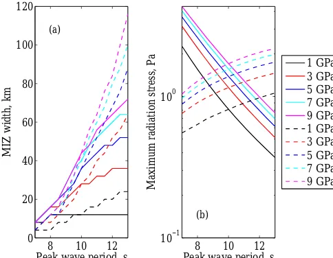
The Young’s modulus is typically somewhere in the range of 1–10 GPa. Williams et al. (2013a) argued for values within the interval 5–7 GPa (depending on the brine volume frac-tion), proposing that the effective elastic modulus, which includes a response to primary, recoverable creep, should cause it to drop somewhat from the relationship of Timco and Weeks (2010). However, Marchenko et al. (2013) de-rived significantly lower values of Young’s modulus (about 1.5 GPa) in Svalbard fjord ice. Marchenko et al. (2017) also measured lower values in the Barents Sea, ranging between 1 and 4 GPa, with no obvious dependance on the brine vol-ume. Therefore, we carry out some tests of the sensitivity of the MIZ width and the maximum WRS to this parameter.
Figure 4 shows the variation of the MIZ width (panel a) and the maximum WRS (panel b) with peak period for dif-ferent values of the Young’s modulus. Since increasing the Young’s modulus increases the attenuation, the waves lose more momentum and so the maximum radiation stress in-creases, and this is clearly seen in Fig. 4b. However, Fig. 4a clearly shows that the MIZ width increases with increas-ing Young’s modulus, so its effect on the breakincreas-ing criterion clearly dominates its effect on the attenuation. The mag-nitude of the maximum radiation stress is of the order of 0.1–1 Pa, which is comparable to the wind stress from 10 to 15 m s−1winds (see Fig. 1d). However, while stresses of this size are significant, they are very much localised around the ice edge as opposed to being applied over large areas (as wind stresses are – see Fig. 1d).
5 10 15 20 25
0 20 40 60 80 100 120 140
Wave period, s
MIZ width, km
(a)
5 10 15 20 25
10−3 10−2 10−1 100 101 102
(b)
Wave period, s
Maximum radiation stress, Pa
1 GPa 3 GPa 5 GPa 7 GPa 9 GPa
Figure 5.Variation of MIZ width(a)and maximum radiation stress
(b)with peak wave period and Young’s modulus for swells of height 3 m. The concentration was 0.7, the thickness was 1 m, and the small-scale cohesion used was 629 kPa. The WIM is not coupled to neXtSIM.
The dashed curves use fully developed seas (Pierson– Moskowitz spectra), whereHs increases with Tp for wave
forcing. Although waves of higher periods are attenuated less, the increasing wave height overcomes this effect and both the MIZ width and maximum radiation stress increases monotonically with peak period.
The solid curves in Fig. 4 are created using an inci-dent wave spectrum based on a Bretschneider spectrum with a constant significant wave height of Hs=4 m. Like with
the dashed curves (fully developed seas), larger values of Young’s modulus cause the MIZ width to increase monoton-ically as peak period increases (in the plotted range of peri-ods). However, whenY =1 GPa, as peak period is increased, the MIZ width is initially 8 km. Then it increases to a maxi-mum of 12 km as the wave frequencies with the most energy are attenuated less, before dropping down to 8 km again as the waves with the most energy, while still being attenuated less strongly, now produce less strain (see Eqs. 22–27).
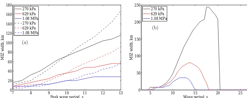
7 8 9 10 11 12 13 0
20 40 60 80 100 120 140 160 180
Peak wave period, s
MIZ width, km
270 kPa 629 kPa 1.08 MPa 270 kPa 629 kPa 1.08 MPa
5 10 15 20 25
0 50 100 150 200 250
Wave period, s
MIZ width, km
270 kPa 629 kPa 1.08 MPa
Figure 6.Variation of MIZ width with peak wave period and small-scale cohesion for(a)wind seas and(b)swells.(a)Dashed curves: Pierson–Moskowitz spectra are used for the forcing. Solid curves: Bretschneider spectrum are used with the significant wave height being 4 m.(b)Swell waves of height 3 m. For both plots, the concentration is 0.7, the thickness is 1 m, and the Young’s modulus used was 5.49 GPa. The WIM is not coupled to neXtSIM.
Figure 6 shows the variation of the MIZ width with the peak period and the small-scale cohesion. Unlike the Young’s modulus, this parameter does not change the attenuation di-rectly, and so the maximum radiation stress is essentially the same for all values of the cohesion (notwithstanding small differences, mainly due to the different MIZ widths, since the attenuation is higher in the MIZ in our model).
The three values chosen are 270 kPa (approximately the flexural strength whenvb=0.1, 274 kPa), 629 kPa
(approxi-mately 2.33×274=638 kPa) and 1.08 MPa (approximately 1.1 MPa, the laboratory value of the cohesion). The results for the MIZ width are significantly different but all are of the correct order of magnitude (a few tens of kilometres). Therefore we will use τ0=629 kPa throughout the rest of
the paper. We will also use a Young’s modulus ofY0=Y∗=
5.49 GPa (i.e. the same value in neXtSIM and the WIM). 5.3 Coupled waves-in-ice results
Figure 7 shows plots of different fields after a 2-day simula-tion with neXtSIM coupled to the WIM. There is no wind, only waves arriving from the left (the initial wave state is shown in Fig. 7a), breaking the ice and pushing it to the right by about 24 km by the end of the 48 h simulation. The ini-tial ice state is the same as in Fig. 1, but with the addition of unbroken ice (Dmax=300 m everywhere wherec >0), as
shown in Fig. 7b. This could correspond to summer ice in the Fram Strait where there can be large floes with large gaps between them (perhaps due to smaller floes melting faster), producing a low concentration.
The resulting MIZ width is about 50 km, which is not un-realistic. Following Eq. (39), there is a cos-squared type of directional spreading applied (16 directions used) and the upper and lower grid cells, which contain land, act to com-pletely absorb the waves. Therefore, in Fig. 7c, the waves are
slightly lower (by about 1 m) near the coast than they are at the centre. In Fig. 7f, thexcomponent of the WRS is plotted – note that while it reaches 1 Pa in the vicinity of the ice edge, it decays exponentially further into the ice. This is reflected in the concentration field (Fig. 7e), which shows that the ice is much more compact at the ice edge. Note that the WRS does not vary significantly in they direction, showing that the boundary conditions used for the waves at the coast do not have too much influence. Also note that the pack and the MIZ, as shown in theDmaxfield (Fig. 7d), are separated by
quite a sharp boundary. This has been preserved by breaking on the mesh in parallel to the breaking on the grid as op-posed to simply interpolatingDmaxback to the mesh after
doing breaking on the grid. Figure 8 shows the same plot as Fig. 7d, but with this latter, more naive, method of coupling. The sharp MIZ-pack boundary has now become extremely diffuse compared to the former scheme.
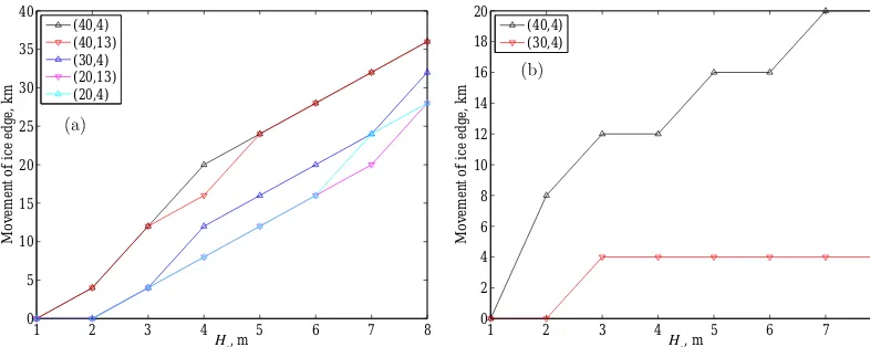
Figure 9 tests the sensitivity of the ice edge motion to the rheological parametersC andτ0L when the ice is subjected to steady waves of varying heights (and periods). In Fig. 9a, the damage is set to 0.9999 everywhere and the ice is broken by the waves, while in Fig. 9b the damage and cohesion are unchanged by ice breakage due to waves. Consequently in Fig. 9a for higher concentrations the internal stress is mainly coming from the ice pressureP, while in Fig. 9bσalso plays a role, since it is not damaged.
0 100 200 300 400 0
50 100 150 200
x, km
y,
km
Hs
, m
0 1 2 3 4 5
0 100 200 300 400
0 50 100 150 200
x, km
y,
km
Dmax
, m
0 150 300
0 100 200 300 400
0 50 100 150 200
x, km
y,
km
Hs
, m
0 1 2 3 4 5
0 100 200 300 400
0 50 100 150 200
x, km
y,
km
Dmax
, m
0 150 300
50 100 150 200 250 300 350 400
50 100 150 200
x, km
y, km c
0 0.5 1
50 100 150 200 250 300 350 400
50 100 150 200
x, km
y, km
log
10
(x
), Pa
−2 −1 0
Figure 7.Waves breaking ice in an idealised experiment (the right-hand, upper and lower lines of the grid cells correspond to land). The wave model, based on Williams et al. (2013a), is coupled to the neXtSIM sea-ice model. The figure shows results after 48 h of steady pushing by a Pierson–Moskowitz wind wave spectrum with significant wave heightHs=5 m (so the peak periodTp=11.2 s), which is arriving from the left. It initially occupies the strip shown in(a), then travels to the right with some directional spreading; the final wave height is shown in(c).(b, d)Initial and final maximum floe size;(e, f)final sea-ice concentration andxcomponent of the wave radiation stress. The ice has initial conditions (constant where there is ice–sea(b)for the initial ice mask):c=0.7,h=1 m,Dmax=300 m, andd=0. Also C=40,
τ0L=4 kPa,τ0S=629 kPa, anddis increased todbreak=0.9999 if the ice is broken.
movement is approximately reduced by half; if it drops even further to 20, then the ice edge no longer moves at all.
However, the large-scale cohesion makes little difference in these simulations where the ice is not failing. Part of the reason for this is that the wave radiation stress is a compres-sive stress, so the stresses need to be larger to move out-side the Mohr–Coulomb envelope than if they were tensile or shear stresses (see Fig. 2: the tensile and shear stresses are near the points of the triangles, while compressive stresses are near their bases).
Some of the runs from Fig. 9 (those with C=40 and τ0L=4 kPa) were repeated with swell waves (of a single fre-quency and direction), with amplitude of 3 m and periods ranging from 10 to 14 s (recalling that the maximum WRS dropped with wave period – Fig. 5b). These were not able to produce any movement of the ice edge though. Therefore,
0 100 200 300 400
0 50 100 150 200
x, km
y,
km
Dmax
, m
0 150 300
1 2 3 4 5 6 7 8 0
5 10 15 20 25 30 35 40
Hs, m
Movement of ice edge, km
(40,4) (40,13) (30,4) (20,13) (20,4)
1 2 3 4 5 6 7 8
0 2 4 6 8 10 12 14 16 18 20
Hs, m
Movement of ice edge, km
(40,4) (30,4)
Figure 9.Maximum movement of the ice edge over 2 days for different pairs(C, τ0L)of the compactness factor and the large-scale cohesion (in kPa). Initial concentration is 0.7, initial thickness is 1 m. Wave forcing is from Pierson–Moskowitz spectra.(a)Damage is set todbreak= 0.9999 if the ice is broken.(b)Damage is unchanged if the ice is broken.
the main influence of swell will be due to their changing of the dynamical and thermodynamical properties of the ice through the ice break-up. As can be seen from Figs. 5–6, they are attenuated less and so they can produce break-up further into the ice than wind waves.
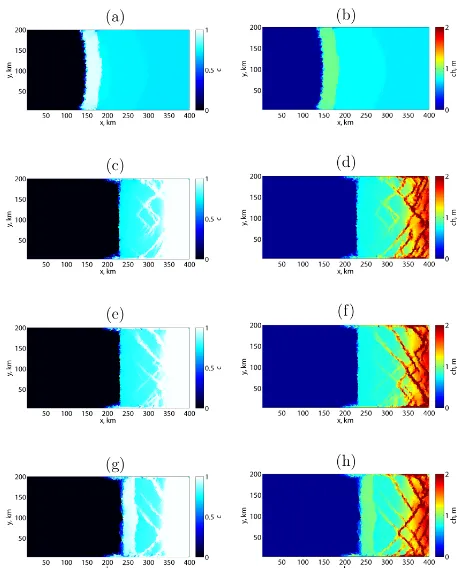
Figure 10 shows the combined effects of wind and waves on the concentration (c) and the effective thickness (ch). For reference, Fig. 10a, b only have waves (5 m waves following a Pierson–Moskowitz spectrum) and no wind (Fig. 10a is the same as Fig. 7e), while Fig. 10c, d have no waves, but only a 15 m s−1wind from the left (as in Fig. 1). This wind speed is consistent with the wind wave spectrum in Fig. 10a, b. Figures 10e–h have both 5 m waves and 15 m s−1wind. All
figures with wind (Fig. 10c–h) exhibit similar ice edge lo-cations, and all show thickening at the far right “coastline”, concentrated in thin ridges. The area over which the ridging is concentrated also seems similar for all the runs. However, while the pattern of thickening between the three runs seems quite different, perturbations to certain parameters in the run with the R1 modification to the EB rheology (Fig. 10g, h), such as dbreak (0.99 and 0.999 were tried) or the minimum
concentration of ice required to cause attenuation (0 or 5 % were tried), produce similar degrees of differences. Therefore we conclude that the actual ridging patterns are not signifi-cant in themselves. The main differences between the R1 run and the other two are therefore in the concentrations at the ice edge (the actual thickness,h, which is not plotted, is constant near the edge). In this run, when the damage is increased if ice breakage occurs, the ice is noticeably more concentrated in a region approximately corresponding to the MIZ. Addi-tionally, the ice edge is more diffuse, possibly due to some feedback effect where if the ice starts to become less concen-trated at the ice edge, the attenuation reduces and therefore so does the wave radiation stress. It then moves more slowly compared to the more concentrated ice, which will experi-ence a higher radiation stress – an effect enhanced by the
high degree of damage, which keeps the more compressed ice quite mobile (as opposed to the run where the rheology is not modified).
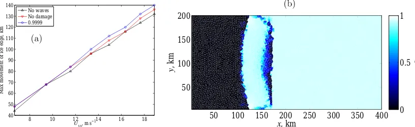
Figure 11a quantifies the results of Fig. 10 with respect to the ice edge location, as well as varying the wind speed. As can be seen from the figure, the waves only increase the movement by 4 km (no damage in the MIZ due to breakage) or 8 km (damage isdbreak=0.9999 in the MIZ when the ice
is broken). That is, the effect of the WRS on the ice edge position is almost completely dominated by the wind stress. When the initial concentration was increased to 95 %, the dif-ference was even less (0–4 km), as then the stress and ice pressureP increased due to their e−C(1−c)factors becoming
closer to 1.
To repeat what we have seen in Fig. 10, when the ice was subjected to on-ice winds in addition to waves, the main ef-fect of linking the damage to the break-up due to waves was that the MIZ region became more highly compressed than the ice immediately further in. In Fig. 11b, we see the effects of off-ice winds on ice preconditioned by swell waves. For the wind speed used in the figure shown (2 m s−1), the wind stress is not able to move the pack ice at all, but the MIZ, which is about 60 km wide and has damagedbreak=0.9999,
has started to detach from the pack. The ice edge has moved about 15 km to the left in the centre of the domain, with less movement at the coasts since there is still some friction there (due to the condition of no slip applied at the top and bottom boundaries).
6 Conclusions and discussions
Figure 10. (a, b)Concentration (c) and effective thickness(ch)after the same experiment as Fig. 7.(c, d)Same as Fig. 1c, d: wind forcing only. Panel(e–h)show results when steady waves (withHs=5 m,Tp=11.2 s, from the left) are applied in addition to the wind forcing. Initial ice conditions are the same as in Fig. 7. In(e, f)the ice rheology is not affected by the ice breakage, but in(g, h)damage is set to
8 10 12 14 16 18 40
50 60 70 80 90 100 110 120 130 140
U10, m s−1
Max movement of ice edge, km
No waves No damage 0.9999
50 100 150 200 250 300 350 400
50 100 150 200
x, km
y, km c
0 0.5 1
Figure 11.Panel(a)shows the maximum movement of the ice edge as a function of wind speed. The different curves show the response to wind forcing only (no waves), wind and waves without changing the EB rheology in the MIZ (no damage), and wind and waves where the damage is set todbreak=0.9999 in the MIZ (0.9999).(b)The effect of swell preconditioning on the response to off-ice winds. Initial conditions: swell of 12 s period and height 3 m is sent into the ice for 24 h, where the ice has constant concentration of 95 % and thickness 1 m, breaking the ice for about 50 km. The damage is set todbreak=0.9999 where the ice is broken. Spatially and temporally constant off-ice wind forcing is then applied for a further 48 h, at a speed of 2 m s−1. The large-scale cohesion is 13 kPa, andC=40.
away from the ice edge. Probably as a consequence of this localisation, overall we found its effects on ice edge loca-tion were quite modest, with the most noticeable effects be-ing seen when a wind wave spectrum was applied steadily to the ice in the absence of wind. Then, depending on the initial concentration, the rheological parameters used and the response to the ice breakage by waves, the radiation stress could produce a movement of the ice edge of between 0 and 36 km over 2 days. However, this experiment is more hypo-thetical since wind waves are by definition associated with wind. Indeed, in the presence of wind, the wind stress domi-nated the WRS with almost no difference in ice edge position between experiments with and without waves. There were differences in the ridging patterns in the presence of waves but these were probably not significant. However, when we modified the damage parameter after ice breakage, additional compression was observed in the MIZ after the ice was bro-ken. Consequently, it seems that the WRS has a very limited effect in general, although it could be a very efficient process to precondition the ice cover and its mechanical properties via the formation of a MIZ area filled with highly damaged ice.
Having said this, however, there are many uncertainties re-garding the WRS, and we have certainly not included all of its potential effects, especially since the wave and ice models are not coupled to the ocean yet. For example, the attenu-ation models are still uncertain (they determine the WRS), and how the partitioning of the WRS between the ice and the ocean should be done is also unknown. On the face of it, if less of the WRS is applied to the ice, it should have even less effect than we find in our current paper. However, perhaps it could then produce similar effects to those discussed and re-ported by Suzuki and Fox-Kemper (2016) and Suzuki et al. (2016) in relation to overturning circulation produced by the
Stokes shear force and thereby change the currents and heat fluxes acting on the ice.
We also highlighted the problem of numerical diffusion of Nfloes due to it being modified by both neXtSIM and
the WIM, and therefore having to be communicated in both directions. We presented a solution to this problem, where Nfloeswas calculated on the neXtSIM mesh each WIM time
step, after interpolating smoother wave fields. While not un-feasible, this is somewhat costly and we will continue to look for alternative solutions.
As touched on in the discussion of the WRS above, we also introduced a simple MIZ rheology by increasing the dam-age where ice was broken, effectively putting the MIZ into free drift, with the addition of the ice pressure, which resists compression. Under compressive wind forcing this led to in-creased compression in the MIZ relative to the pack ice in its vicinity. This modification also influenced the ice flow when off-ice winds were applied to ice that had previously been broken by swell waves. At lower wind speeds, the MIZ was able to be move relatively freely with the wind, while the pack was still stationary. These effects would undoubtedly be reduced in magnitude were a rheology that represented true granular flow to be used, but could still occur. However, it is difficult to know for certain without the existence of such a rheology. Direct numerical simulations such as those done by Herman (2016) could possibly reproduce some of the effects observed here. Similarly, the granular temperature model of Feltham (2005) could be tried, although this would be limited to flow regimes where large force networks are not expected to be present.
impact. In addition, the study of Horvat et al. (2016) sug-gests that including the thermodynamic effects of ice break-age by waves could be important. We are also currently im-plementing the more conservative lateral melting model of Steele (1992) in our model to include this effect to some extent. With simulations using a WIM coupled to a stand-alone version of CICE-E, which contains the model of Steele (1992), Bennetts et al. (2017) found that the concentration in the vicinity of the Antarctic ice edge could drop by a modest amount (of the order of 10 %) in the summer. However, this could also change with coupling to an ocean model, as well as if a different parameterisation that reflects the increased lateral melting of larger floes was used.
Code and data availability. These data are not publicly available. The model code is not released yet, since it is still being developed, and lacks the full documentation.
Author contributions. The writing of the paper and implementation of the coupling between the WIM and neXtSIM was lead by TW, with formative discussions from PR and SB guiding the progression of the writing. PR also helped with the writing itself, and in addition SB helped to implement the coupling.
Competing interests. The authors declare that they have no conflict of interest.
Acknowledgements. This work was primarily supported by the neXtWIM project (Norwegian Research Council grant no 244001). Earlier WIM code development was also supported by the SWARP project (EU-FP7 project 607476) and ONR Global project N62909-14-1-N010. We were also helped by discussions with Einar Ólason and Aleksey Marchenko. Finally we would like to thank our reviewers and editor for their helpful comments.
Edited by: Jennifer Hutchings Reviewed by: two anonymous referees
References
Ardhuin, F., Sutherland, P., Doble, M., and Wadhams, P.: Ocean waves across the Arctic: Attenuation due to dissipation domi-nates over scattering for periods longer than 19s., Geophys. Res. Lett., 43, 5775–5783, https://doi.org/10.1002/2016GL068204, 2016.
Ardhuin, F., Stopa, J., Chapron, B., Collard, F., Smith, M., Thom-son, J., Doble, M., Blomquist, B., PersThom-son, O., Collins, III, C. O., and Wadhams, P.: Measuring ocean waves in sea ice us-ing SAR imagery: A quasi-deterministic approach evaluated with Sentinel-1 and in situ data, Remote Sens. Environ., 189, 211– 222, https://doi.org/10.1016/j.rse.2016.11.024, 2017.
Bagnold, R. A.: Experiments on a gravity-free dispersion of large solid spheres in a newtonian fluid under shear, Proc. R. Soc. A, 225, 49–63, https://doi.org/10.1098/rspa.1954.0186, 1954. Bennetts, L. G. and Squire, V. A.: On the
calcula-tion of an attenuacalcula-tion coefficient for transects of ice-covered ocean, Proc. Roy. Soc. Lond. A, 468, 136–162, https://doi.org/10.1098/rspa.2011.0155, 2012.
Bennetts, L. G., O’Farrell, S., and Uotila, P.: Brief commu-nication: Impacts of ocean-wave-induced breakup of Antarc-tic sea ice via thermodynamics in a stand-alone version of the CICE sea-ice model, The Cryosphere, 11, 1035–1040, https://doi.org/10.5194/tc-11-1035-2017, 2017.
Bouillon, S. and Rampal, P.: Presentation of the dynamical core of neXtSIM, a new sea ice model, Ocean Model., 91, 23–37, https://doi.org/10.1016/j.ocemod.2015.04.005, 2015a.
Bouillon, S. and Rampal, P.: On producing sea ice deformation data sets from SAR-derived sea ice motion, The Cryosphere, 9, 663– 673, https://doi.org/10.5194/tc-9-663-2015, 2015b.
Dansereau, V., Weiss, J., Saramito, P., and Lattes, P.: A Maxwell elasto-brittle rheology for sea ice modelling, The Cryosphere, 10, 1339–1359, https://doi.org/10.5194/tc-10-1339-2016, 2016. Doble, M. J. and Bidlot, J.-R.: Wavebuoy
measure-ments at the Antarctic sea ice edge compared with an enhanced ECMWF WAM: progress towards global waves-in-ice modeling, Ocean Model., 70, 166–173, https://doi.org/10.1016/j.ocemod.2013.05.012, 2013.
Dumont, D., Kohout, A. L., and Bertino, L.: A wave-based model for the marginal ice zone including a floe breaking parameterization, J. Geophys. Res., 116, 1–12, https://doi.org/10.1029/2010JC006682, 2011.
Feltham, D. L.: Granular flow in the marginal ice zone, Philos. T. R. Soc. A, 363, 1677–1700, 2005.
Frederking, R. M. W. and Svec, O. J.: Stress-relieving techniques for cantilever beam tests in an ice cover, Cold Reg. Sci. Technol., 11, 247–255, 1985.
Fung, Y.: Foundations of Solid Mechanics, Prentice-Hall Inc, En-glewood Cliffs, New Jersey, 1965.
Guo, T. and Campbell, C. S.: An experimental study of the elastic theory for granular flows, Phys. Fluids, 28, 083303, https://doi.org/10.1063/1.4961096, 2016.
Herman, A.: Sea-ice floe-size distribution in the context of sponta-neous scaling emergence in stochastic systems, Phys. Rev. E, 81, 066123, https://doi.org/10.1103/PhysRevE.81.066123, 2010. Herman, A.: Influence of ice concentration and floe-size distribution
on cluster formation in sea-ice floes, Cent. Eur. J. Phys., 10, 715– 722, https://doi.org/10.2478/s11534-012-0071-6, 2012. Herman, A.: Shear-Jamming in two-dimensional granular materials
with power-law grain-size distribution, Entropy, 15, 4802–4821, https://doi.org/10.3390/e15114802, 2013.
Herman, A.: Discrete-Element bonded-particle Sea Ice model DE-SIgn, version 1.3a – model description and implementation, Geosci. Model Dev., 9, 1219–1241, https://doi.org/10.5194/gmd-9-1219-2016, 2016.
Hibler, III, W. D. and Leppäranta, M.: MIZEX 83 mesoscale sea ice dynamics: initial analysis, in: MIZEX: Bull. IV, U.S. Army Cold Reg. Res. and Eng. Lab., 1984.