www.ocean-sci.net/9/19/2013/ doi:10.5194/os-9-19-2013
© Author(s) 2013. CC Attribution 3.0 License.
Ocean Science
Assimilation of sea-ice concentration in a global climate model –
physical and statistical aspects
S. Tietsche1,2,*, D. Notz1, J. H. Jungclaus1, and J. Marotzke1
1Max Planck Institute for Meteorology, Bundesstr. 53, 20146 Hamburg, Germany
2International Max Planck Research School on Earth System Modelling, Hamburg, Germany *now at: NCAS-Climate, University of Reading, Reading, UK
Correspondence to: S. Tietsche ([email protected])
Received: 30 June 2012 – Published in Ocean Sci. Discuss.: 19 July 2012
Revised: 20 November 2012 – Accepted: 4 December 2012 – Published: 15 January 2013
Abstract. We investigate the initialisation of North-ern Hemisphere sea ice in the global climate model ECHAM5/MPI-OM by assimilating sea-ice concentration data. The analysis updates for concentration are given by Newtonian relaxation, and we discuss different ways of spec-ifying the analysis updates for mean thickness. Because the conservation of mean ice thickness or actual ice thickness in the analysis updates leads to poor assimilation perfor-mance, we introduce a proportional dependence between concentration and mean thickness analysis updates. Assim-ilation with these proportional mean-thickness analysis up-dates leads to good assimilation performance for sea-ice con-centration and thickness, both in identical-twin experiments and when assimilating sea-ice observations. The simulation of other Arctic surface fields in the coupled model is, how-ever, not significantly improved by the assimilation. To un-derstand the physical aspects of assimilation errors, we con-struct a simple prognostic model of the sea-ice thermody-namics, and analyse its response to the assimilation. We find that an adjustment of mean ice thickness in the analy-sis update is essential to arrive at plausible state estimates. To understand the statistical aspects of assimilation errors, we study the model background error covariance between ice concentration and ice thickness. We find that the spatial structure of covariances is best represented by the propor-tional mean-thickness analysis updates. Both physical and statistical evidence supports the experimental finding that as-similation with proportional mean-thickness updates outper-forms the other two methods considered. The method de-scribed here is very simple to implement, and gives results that are sufficiently good to be used for initialising sea ice in a global climate model for seasonal to decadal predictions.
1 Introduction
For skillful seasonal to decadal predictions, good ini-tial conditions of atmosphere–ocean global climate models (AOGCMs) are of paramount importance. So far, global pre-diction studies have been restricted to the initialisation of the oceanic and atmospheric state (e.g., Smith et al., 2007; Pohlmann et al., 2009). However, slow surface processes might constitute a substantial source of untapped predictabil-ity (Hurrell et al., 2009; Shepherd et al., 2011). One of the most important of these surface processes is arguably the existence of sea ice at high latitudes. Holland et al. (2010) and Blanchard-Wrigglesworth et al. (2011a) have shown that Arctic sea ice has inherent predictability of up to two years. Moreover, anomalies in Arctic sea ice can have an influ-ence far beyond the Arctic by changing the large-scale at-mospheric circulation (Honda et al., 2009; Budikova, 2009; Francis and Vavrus, 2012) and the oceanic thermohaline circulation (Koenigk et al., 2006; Levermann et al., 2007). Hence, the initialisation of sea ice in an AOGCM with suit-able data assimilation techniques is an important step to-wards more skillful seasonal to decadal predictions. Here, we investigate data assimilation techniques for the initial-isation of Northern Hemisphere sea ice in the AOGCM ECHAM5/MPI-OM.
sea-ice data assimilation suffers from a large uncertainty about the true thickness. Initial conditions derived from the assimilation inherit this uncertainty, which in turn severely limits the reliability of sea-ice predictions.
Previous studies have demonstrated that the assimilation of observed sea-ice concentration in ice–ocean models im-proves the simulated concentration (Lisæter et al., 2003; Lindsay and Zhang, 2006; Stark et al., 2008). However, the improvement in ice thickness is not straightforward, and Duli`ere and Fichefet (2007) emphasised that the assimilation can easily deteriorate the model performance if inappropriate assimilation techniques are chosen.
These findings from ice concentration assimilation in ice– ocean models forced by atmospheric surface conditions can-not be directly transferred to ice-concentration assimilation in AOGCMs, because in AOGCMs the atmospheric surface conditions are not necessarily consistent with the assimilated sea-ice state. Rather, they develop interactively from large-scale dynamics and from local interaction with the sea-ice state. This makes the impact of ice-concentration assimila-tion on ice thickness less obvious than in ice–ocean models and calls for dedicated studies on sea-ice data assimilation in an AOGCM. To our knowledge, the only such published study is by Saha et al. (2010), who did not describe the im-pact of the ice concentration assimilation on ice thickness.
Here, we assimilate observations of Northern Hemisphere sea-ice concentration and compare different methods of prescribing changes in mean ice thickness associated with changes in ice concentration during the assimilation step. We systematically assess the assimilation performance both for concentration and thickness, and use conceptual arguments to explain the differences in assimilation performance.
The rest of the paper is organised as follows: Sect. 2 describes the global climate model used for this study, in particular the sea-ice component. Section 3 introduces the sea-ice data assimilation methods which we use to investi-gate feasibility of sea-ice data assimilation. The assimilation performance is evaluated first in identical-twin experiments (Sect. 4) and then with actual observations of sea-ice concen-tration (Sect. 5). Section 6.1 uses both a simple model and an AOGCM case study to develop a conceptual understanding of assimilation errors, while Sect. 6.2 analyses the model er-ror statistics. Section 7 presents conclusions.
2 The coupled global climate model
2.1 The atmosphere and ocean models
Our AOGCM consists of the atmosphere component ECHAM5 (Roeckner et al., 2003) with a T31 horizontal resolution and 19 vertical levels, and the ocean component MPI-OM (Marsland et al., 2003) with a curvilinear grid that has a horizontal resolution of 50–200 km in the Arctic and 40 vertical levels. The time step of the atmosphere model
is 40 min, the time step of the ocean and sea-ice models is 144 min. The ocean and atmosphere exchange surface fields once a day before the first time step. The model setup is a coarse-resolution version of the IPCC-AR4 model described by Jungclaus et al. (2006).
2.2 The sea-ice model
The sea-ice model in ECHAM5/MPI-OM is based on Hi-bler III (1979) and Semtner (1976). It consists of three prog-nostic equations for the mean ice thicknesshm(x, y, t), the ice concentrationC(x, y, t), and the ice velocityv(x, y, t ):
∂thm= ∇ ·(hmv)+Sh (1)
∂tC= ∇ ·(Cv)+SC (2)
∂tv= −f (k×v)−g∇ζ+ τa
ρihm
+ τo
ρihm
+ ∇ ·σ. (3) The divergence terms on the right-hand side of Eqs. (1) and (2) describe the redistribution of ice volume and concentra-tion by advecconcentra-tion with ice velocityv.ShandSCare the
ther-modynamic sources of mean thickness and concentration, re-spectively, which describe local melting and freezing. The change of ice velocityv=(vx, vy) is determined by the mo-mentum balance of Eq. (3), wheref is the Coriolis parame-ter,kthe vertical unit vector,gthe Earth’s gravitational ac-celeration,ζthe sea-surface height above sea-level,ρithe ice density,τa/othe stress of wind from above and of ocean cur-rent from below, andσthe sea-ice internal stress tensor. The terms on the right-hand side of Eq. (3) from left to right cor-respond to forces that originate in the Coriolis effect, the tilt of the sea-surface, the drag from atmosphere and ocean, and internal sea-ice stresses.
These equations are based on the model assumption that within a grid cell, a fractionCof the area is covered by thick ice with the constant actual thicknessht, and the remaining fraction 1−Cof the area is open water. The actual thickness htis connected to the mean ice thicknesshmby
hm=Cht. (4)
It is further assumed that the sea-water in a grid cell that contains sea ice is always at a representative sea-water freez-ing temperature of−1.9◦C. Thus, any heat flux imbalance
over either the ice-covered or the open-water part of the grid cell is immediately converted into ice growth or melt, and so the thermodynamic source of mean ice thickness in Eq. (1) is given by:
Sh=Cgi+(1−C)gw. (5)
from the surface energy balance of the coupled model, as-suming a linear temperature profile within the ice (Semtner, 1976).
The thermodynamic source term for ice concentrationSC
is parametrised in terms of the ice growth rates according to Hibler III (1979):
SC=2 (gw)
gw
h0(1−C)+2 (−Sh) C
2hmSh, (6)
with2the Heaviside step function (i.e.2(x)=1 ifx≥0, 2(x)=0 ifx <0). The first term on the right-hand side of Eq. (6) is active when new ice forms from open water; the parameterh0=0.5 m is chosen such that open water freezes over within a few days if there is strong ice growth. The second term approximates the decrease in ice concentration when thick ice melts, assuming that the thickness of the ice floe is distributed linearly between 0 and 2ht. A critical dis-cussion of Eq. (6) is provided by Mellor and Kantha (1989).
3 Sea-ice data assimilation approach
In this study, we utilise daily data of Arctic sea-ice concen-tration. In Sect. 4, these data are derived from model output, whereas in Sect. 5 they are derived from satellite observa-tions. For the concentration analysis updates, we choose here the simplest possible approach: the Newtonian relaxation of the model state towards observations (Lindsay and Zhang, 2006). This approach is feasible here since sea-ice concen-tration observations are both dense and relatively reliable. The analysis updates of other sea ice-related variables like mean ice thickness, sea-surface temperature and sea-surface salinity are derived from the concentration analysis updates as described in Sects. 3.2 and 3.3.
We remind the reader that Newtonian relaxation is the sim-plest conceivable data assimilation scheme. It does not ac-count for spatial correlation in model and observations; nor does it account for multivariate covariances, unless they are explicitly prescribed. Therefore, the state estimates obtained by this simple method should always be critically evaluated. For an overview of state-of-the-art data assimilation tech-niques, which in general provide far more consistent state es-timates, see for instance Kalnay (2003). Nevertheless, there is one major advantage of the Newtonian Relaxation: its im-plementational complexity and computational costs are or-ders of magnitude smaller than those of more complex meth-ods. If this simple approach delivers a state estimate that is good enough for the application at hand, we argue that it can be a very useful alternative to full-fledged assimilation meth-ods. In our case, the application is the initialisation of sea ice in a global climate model for seasonal to decadal climate predictions. There, the usefulness of the initialisation can be easily inferred from the change in predictive skill that it pro-vides.
We perform long assimilation runs for the period 1979–2007, spanning almost the entire satellite observational record of Northern Hemisphere sea-ice concentration. We primarily consider the global performance of sea-ice data assimilation, averaged over different regions and different years, rather than focus on specific case studies. On the one hand, this complicates the attribution of failure or success of a method to physical causes, since we deal with the average over a plethora of different local conditions. On the other hand, we can verify that there are no spurious drifts in the AOGCM induced by the sea-ice data assimilation and that the perfor-mance is robust over a range of climatic conditions.
In the following, we use the notation of Bouttier and Courtier (1999). For any variable x, we denote the model background state byxband the observed state byxo. Every time an assimilation step is performed, the departure of the modelled statexbfrom the observed statexo is calculated, and a correction1xis computed that depends on this depar-ture. The correction1xis called the analysis update, and the corrected statexa=xb+1xis called the analysis.
3.1 Analysis updates of ice concentration
We obtain the analysed sea-ice concentrationCaonce a day by correcting the model background concentrationCb with an analysis update1Cthat corresponds to Newtonian relax-ation towards observed valuesCo:
Ca=Cb+1Cwith1C=KN
Co−Cb
. (7)
The scalar constantKNdetermines the strength of the anal-ysis update. This approach is akin to data assimilation by nudging, where the same analysis update would be applied at each time step of the model. For all our experiments, we choose KN=0.1. Without model interaction, the analysis update in Eq. (7) withKN=0.1 applied once a day leads to the exponential relaxation of an initial departure of the model background state from the observation on a relaxation time scale ofTR=10 days. Thus, the time scale of the
assimila-tion matches the time scale on which large-scale changes in sea ice can occur. Section 6.2 discusses further implications of the choice ofKN.
3.2 Analysis updates of mean ice thickness
We consider analysis updates of mean ice thicknesshmas a function of analysis updates of ice concentration:
It is to be expected that this approach works well close to the ice edge, where concentration is very variable, and corre-lation between concentration and thickness is strong. In the central Arctic, however, ice concentration is almost always close to 100 %, and the correlation between concentration and thickness is weak. There, we cannot expect this approach to correct ice thickness from concentration data effectively.
As we will see in Sects. 4 and 5, the assimilation error dif-fers substantially between different choices for the functional dependencef, and in Sects. 6.1 and 6.2 we will discuss pos-sible sources of assimilation errors in detail. We introduce and discuss the following three choices:
3.2.1 Analysis updates with conserved mean thickness (CMT)
With this method, the analysis update of mean ice thickness hmis always zero, no matter the value of the concentration analysis update:
1hm=0. (9)
The analysed actual ice thicknesshat is then given byhat =
hbtCb/Ca. From idealised experiments with prescribed per-turbations in thermodynamic atmospheric forcing, Duli`ere and Fichefet (2007) concluded that this is the best approach when model error is mainly due to ice advection.
3.2.2 Analysis updates with conserved actual thickness (CAT)
We assume that the model has the correct actual ice thickness ht, and demand that1ht≡hat−hbt
!
=0. Applying Eqs. (4) and (8), we see that this is guaranteed if we choose:
1hm=hbt1C, (10)
wherehbt =hbt(x, y, t )is the spatially and temporally vary-ing actual thickness in the model background. Thus, for the same concentration analysis update, mean-thickness analysis updates will be small for low background actual thickness, and large for high background actual thickness. Duli`ere and Fichefet (2007) found that this method performs best when model error is mainly due to ice thermodynamics.
3.2.3 Proportional mean thickness analysis updates (PMT)
Duli`ere and Fichefet (2007) report best assimilation results for a combination of CMT and CAT, depending on whether errors are related to errors in the thermodynamic or the dy-namic forcing of the sea ice. However, in an AOGCM the attribution of errors in the sea-ice state to either dynamical or thermodynamical processes is not practicable. Hence, we propose a simple new scheme that – as we will show – per-forms well independent of the source of the errors. This is
a scheme where the mean-thickness analysis updates have a fixed proportionality to the concentration analysis updates:
1hm=h∗1C. (11)
The proportionality constanth∗is a free parameter. In our ex-periments, we use a value ofh∗=2 m. That means that for a concentration update of 1 % we change the mean ice thick-ness by 2 cm. However, we find that the assimilation perfor-mance considered in Sects. 4 and 5 is not very sensitive to changingh∗in the range 0.5 m≤h∗≤4 m. Our choice ofh∗ is supported by the frequency of occurrence of mean thick-ness and concentration in the AOGCM (see Sect. 6.1) and the model background error covariance between concentra-tion and thickness diagnosed from the AOGCM (Sect. 6.2). 3.3 Analysis updates of sea-surface temperature
and salinity
Growth and melt of sea ice are strongly coupled to the prop-erties of the sea-water directly below and adjacent to the ice. Thus, sea-ice data assimilation schemes for a model with a prognostic ocean need to find a satisfying solution to adjust sea-surface salinity (SSS) and sea-surface temperature (SST) when changing the sea-ice state through the analysis updates. In ECHAM5/MPI-OM, the assimilation of SST in the presence of sea ice is implicitly provided by the assumption of thermodynamic equilibrium between sea ice and the water in the ocean surface layer. If sea ice is present in the obser-vations, but not in the model, positive analysis updates of ice concentration merely lead to a decrease in SST until the freezing point is reached. In this case, analysis updates for sea ice are effectively zero, while we have negative analy-sis updates of SST. As soon as ice starts to form, SST stays constant at the freezing temperature, and the analysis updates change only the sea-ice concentration and thickness.
The SSS plays an important role for the establishment or inhibition of oceanic convection in the presence of sea ice. If there is convection, the entrainment of warm wa-ter from below during the deepening of the surface mixed layer can inhibit ice growth considerably (see, for instance, Lemke, 1987). Since growth and melt of sea ice provide sub-stantial freshwater fluxes into the ocean surface water, the treatment of SSS in the analysis update will strongly inter-act with the sea-ice analysis. The charinter-acter of this interac-tion, however, is very variable and depends on the specific local conditions. Since the covariance between ice concen-tration and SSS shows such a high degree of complexity (Lisæter et al., 2003), it is not feasible to prescribe a global time-independent functional relation between the analysis updates that exploits the existing covariance structures.
4 Assimilating sea-ice data in identical-twin experiments
4.1 Rationale and method
When assimilating observed sea-ice concentration in an AOGCM, we face two basic problems: (i) the ice thickness and the state of the ocean below sea ice are poorly observed, hence we cannot determine if the assimilation improves those variables, and (ii) we cannot decide if problems in the assim-ilation are due to drawbacks in the assimassim-ilation scheme or due to model biases.
Those issues can be addressed in a so-called “identical-twin” or “perfect-model” study. In the data assimilation con-text, this means that we treat model output from a reference run as observations, and assimilate it back into a different run of the same model. When both model runs start from differ-ent but climatologically equivaldiffer-ent initial conditions and are exposed to the same external forcing, the model is perfect with respect to the reference-run observations. This allows us to disentangle the effects of model bias and data assimila-tion method and to answer the quesassimila-tion, “If the model were perfect, would we be able to initialise it successfully with a given data assimilation approach?”.
The reference run R is started from a long control run with preindustrial conditions, and is then exposed to the ob-served greenhouse-gas forcing from 1900 onwards. In the reference run, the overall decrease of Northern Hemisphere sea-ice extent is comparable to observations, although the re-treat of summer-time sea ice is somewhat underestimated. A detailed description of the deficiencies of the IPCC-AR4 ver-sion of this model in simulating Northern Hemisphere sea ice is given by Koldunov et al. (2010).
We obtain an equivalent but different realisation of nat-ural climate variability by starting a second runP in 1979 with exactly the same model setup, but from slightly per-turbed initial conditions. The applied perturbation is a time shift of the model state by one day, and is hence compara-tively small. However, the perturbation is quickly amplified by chaotic processes, so that important large-scale modes of climate variability, like ENSO, the slow components of the Atlantic meridional overturning circulation, and interannual variations in sea-ice cover are out of phase between the two runs.
The assimilation runAstarts from the same initial condi-tions as the perturbed runP, but assimilates the ice concen-tration from the reference runR. The time period considered is 1979 to 2007, so that we can later compare the assimilation of ice concentration from model output to the assimilation of ice concentration from satellite observations.
To quantify the usefulness of the data assimilation, we measure the mismatch of a climate variableXbetween any two time series with the root mean square differences be-tween the two time series:
δXT1T2= q
h XT1(t )−XT2(t ) 2
i. (12)
The expectation valueh·iis meant to be taken over time for aggregated quantities like Northern Hemisphere sea-ice ex-tent, and over time and space for field variables like sea-ice concentration.
Using Eq. (12), we can compare the natural variability δXRP with the assimilation error δXRA. Only if δXRA< δXRP does the assimilation actually improve the initialisa-tion ofXin the model. For a perfect initialisation ofX, we would haveδXRA=0.
4.2 Results
For seasonal to decadal predictions of sea ice, the total ice volume and the total area covered are arguably the most important parameters (Holland et al., 2010; Blanchard-Wrigglesworth et al., 2011b). They are closely related to lo-cal ice thickness and ice concentration: ice volume is propor-tional to the sum of the mean thickness for all grid cells, and ice extent is the area sum of all grid cells with ice concen-tration higher than 15 %. In the following, we will therefore quantify the improvement brought by the data assimilation by discussing errors in ice volume and ice extent alongside root mean square errors (RMSE) of concentration and thick-ness.
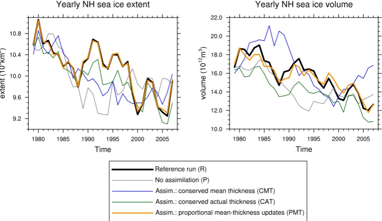
Figure 1 shows how successfully the different assimilation schemes allow the assimilation run Ato match the annual mean sea-ice extent and sea-ice volume of the reference run R. The reference run has generally decreasing sea-ice extent and sea-ice volume in response to the warming background climate. Additionally, there are year-to-year variations as well as decadal-scale variations in the sea-ice state. For in-stance, between 1988 and 1991 sea-ice extent increases, stays relatively high until 1998, and then drops sharply to the low-est value of the time series in 2000. We consider a sea-ice data assimilation successful only if (i)Ahas the same clima-tology asR, i.e. the multi-year running means are the same, (ii)Ashows similar decadal-scale anomalies asR, and (iii) Ahas year-to-year changes comparable toR.
The CMT assimilation scheme fails in all three criteria: it does not reproduce the negative trend in sea-ice volume, the period between 1984 and 1992 that should see a negative anomaly in sea-ice volume actually has a positive anomaly, and the small year-to-year fluctuations are not captured at all. The CAT run has a negative bias, but reasonably cap-tures year-to-year and decadal variations. Finally, the PMT run meets all three criteria set above, and by far provides the best assimilation performance.
Fig. 1. Annual mean sea-ice extent (left) and sea-ice volume (right) in the Northern Hemisphere for the identical-twin study. Shown are the reference run (black), the perturbed run with no assimilation (grey), and the assimilation runs (colours) that assimilate sea-ice concentration from the reference run. The corresponding time-averaged global extent and volume errorsδSIE andδSIV are given in Table 1.
Table 1. Average assimilation error after Eq. (12) for annual mean Arctic ice volume and extent in the twin study (first and second column; cp. Fig. 1) and for annual mean Arctic ice extent when compared to observations (third column; cp. Fig. 3).
Twin study Observations
δSIV(1012m3) δSIE(1012m2) δSIE(1012m2)
No assimilation 2.1 0.56 0.35
CMT assimilation 2.4 0.41 0.60
CAT assimilation 1.8 0.25 0.51
PMT assimilation 0.6 0.03 0.07
that only PMT reduces the error in sea-ice volume far below the level of natural variability.
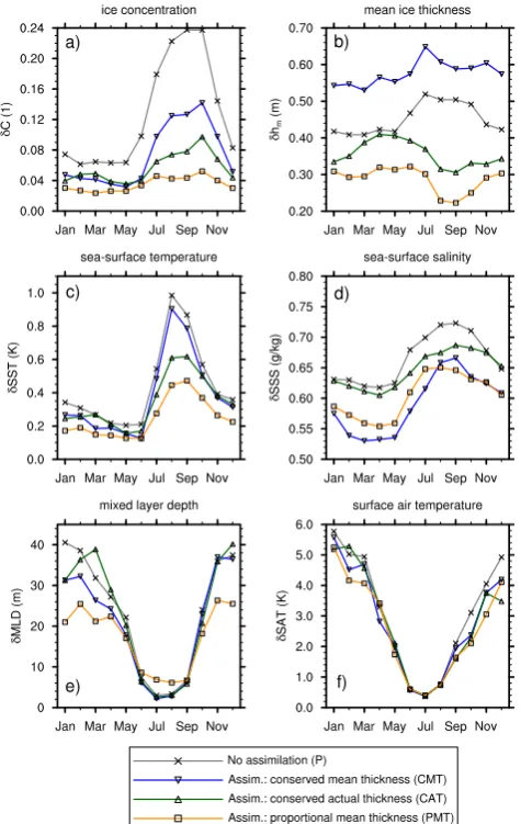
To analyse the seasonal cycle of the assimilation errors, we calculate the discrepancy in concentrationδC and mean thicknessδhmfor the Arctic Ocean with Eq. (12), taking the time mean separately for each month of the year (Fig. 2a and b). Since the Arctic Ocean is essentially ice-covered during winter, even the no-assimilation run exhibits only small nat-ural variations in sea-ice concentration, withδCRP≈5–8 %. The summer melt, however, is much more variable, and con-centration variability in the no-assimilation run reaches 24 % in September and October. Clearly, all assimilation methods are able to significantly reduce the concentration discrepancy δC, although there are marked differences between the meth-ods. The CMT gives the worst performance, and the PMT gives the best performance, reducing concentration error to about 5 % year-round.
The error in mean thickness δhm is shown in Fig. 2b. The natural variabilityδhm(R, P )is about 40 cm in winter and about 50 cm in summer. It is evident that the CMT does not decrease, but even increases the error of mean ice thickness, i.e.δhm(R, P ) < δhm(R, A). This is quite a dramatic failure of the data assimilation method. In Sects. 6.1 and 6.2 we will see that there are good conceptual arguments why the CMT is not a suitable assimilation method in an AOGCM.
The two other methods (CAT and PMT) successfully re-duce the thickness error. Again, PMT has the lowest thick-ness error; it is about 25–30 cm year-round. Note that the as-similation is most successful in summer, as it halves the error in the mean ice thickness compared to the natural variability. We shall also assess the impact of the sea-ice data as-similation on Arctic climate variables that are closely re-lated to sea ice, but not directly changed by the assimila-tion procedure: the Arctic Ocean SST and SSS, the Arctic Ocean mixed-layer depth, and the Arctic surface air temper-ature (SAT). In our simple assimilation method, these fields are constrained neither by observations nor by statistical rela-tionships with analysis updates of sea-ice concentration, and so it is important to check whether our assimilation method introduces unexpected anomalies in these fields.
Fig. 2. Average point-wise root mean square error for each month over the Arctic Ocean for (a) sea-ice concentration, (b) sea-ice mean thickness (c) sea-surface temperature, (d) sea-surface salin-ity, (e) ocean mixed layer depth, and (f) surface air temperature. All errors are obtained from the differences to the reference run of the identical-twin experiments.
0.6 to 0.7 g kg−1as the level of natural variability (Fig. 2d). This demonstrates that assimilation of sea-ice concentration with our approach is not very successful in constraining other variables in the climate model. The Arctic Ocean mixed-layer depth (Fig. 2e) shows even less positive impact of the assimilation. While assimilation with the PMT method re-duces mixed-layer-depth error over the winter months, it in-creases the error over the summer months. Finally, for Arctic SAT we find a slight improvement caused by the assimila-tion between September and March, but little effect in sum-mer months (Fig. 2f). In summary, we note that (i) the as-similation improves the considered non-sea-ice fields only marginally, but does not introduce unexpected anomalies in these fields, and (ii) the PMT assimilation performs better
than the CMT and CAT methods also for the non-sea-ice fields considered.
5 Assimilating sea-ice observations
We now investigate how successfully we can assimilate satel-lite observations of sea-ice concentration into the coupled cli-mate model. The observations are derived from Nimbus-7 SMMR and DMSP SSM/I passive microwave data, pro-cessed by the NSIDC with the NASA team algorithm (Cav-alieri et al., 2008). Temporal resolution of the data is every two days, which we interpolate to daily values. The horizon-tal resolution is 25 km, which we interpolate to the model resolution of about 50–200 km. For an estimate of uncer-tainty in the sea-ice concentration observations, the reader may refer to Tonboe and Nielsen (2010), who arrive at an error estimate of around 10 % on average. The assimilation methods we employ in this section are exactly the same as in the identical-twin study. We will again show ice extent along-side with concentration RMSE as a performance metric. Note that the observational uncertainties in year-to-year changes in ice extent are only in the order of 104km2(NSIDC user ser-vice, personal communication), and are therefore negligible when discussing observed year-to-year changes in the order of 106km2.
5.1 Ice concentration
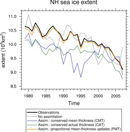
From Fig. 3 we see that the annual mean state of ice extent in ECHAM5/MPI-OM without data assimilation is reasonably close to the observed state. Of course, there are marked dif-ferences between the free model and the observations that are caused by natural variability – for instance, at the observed extreme extent minimum in 2007 the model actually has a temporary extent maximum.
Comparing Fig. 3 with Fig. 1, we see that the conclusions regarding the performance of the different methods are the same as in the identical-twin study: CMT fails as a sea-ice data assimilation approach in all quality criteria, CAT repro-duces natural variability somewhat, but has a biased mean state, and PMT has both an acceptable mean state and repro-duces natural variability satisfyingly. Considering the time-averaged measure for the assimilation error in sea-ice extent, δSIE, we see that only PMT is able to reduceδSIE below the no-assimilation case (see Table 1).
Fig. 3. Annual mean ice extent in the Northern Hemisphere from observations (black), a model run with no assimilation (grey), and from the different assimilation methods (colours). The correspond-ing time-averaged global extent errorsδSIE are given in Table 1.
ice-concentration error that are very similar to the results of assimilating output of the same model. This indicates that the assimilation performance for sea-ice concentration is de-termined more by deficiencies in the assimilation techniques rather than by model biases.
5.2 Ice thickness
There are currently only few large-scale ice thickness mea-surements available (Rothrock and Wensnahan, 2007; Kwok et al., 2009). For a direct comparison of the simulated ice thickness with observations, we need validated observations that cover the whole Arctic Ocean. The only such data set available to us are ice thickness measurements from the ICE-Sat laser altimeter between 2005 and 2008 processed by Yi and Zwally (2010). These data have complete coverage of mean sea-ice thickness data north of 65◦N. Unfortunately, they are only available for a few discontinuous months, when the laser altimeter on the satellite was in operation. Due to the limited temporal coverage of direct observations, we also compare our assimilation results to the PIOMAS reanalysis of Arctic sea-ice volume, which has been thoroughly val-idated against all available observations of ice thickness (Schweiger et al., 2011).
As shown in Fig. 5, there are differences between the ICE-Sat and PIOMAS ice volume estimates of up to 3000 km3, which are, however, mostly compatible with their respec-tive uncertainties as estimated by Kwok et al. (2009) and Schweiger et al. (2011). The relative anomaly of the annual
Fig. 4. The average point-wise error in sea-ice concentration for the Arctic Ocean for each month of the year. All errors are obtained from the differences to the observed concentration fields.
sea-ice minimum in 2007 with respect to the previous years is a prominent feature in both data sets.
The no-assimilation run with ECHAM5/MPI-OM has too low an ice volume throughout. All assimilation methods bring the ice volume closer to both ICESat and PIOMAS estimates. Nevertheless, the CMT assimilation run performs less well regarding two aspects: first, it consistently over-estimates the seasonal cycle in comparison with PIOMAS; and second, it does not show anomalously low volume in 2007 with respect to the previous years. The CAT and PMT methods on the other hand are always – except for ICESat data in March 2007 – within the error bars of both PIOMAS and ICESat volume estimates, and they do capture the 2007 anomaly.
6 Understanding assimilation errors
6.1 Physical aspects – local sea-ice growth rates
We have seen in Sect. 4.2 that assimilating sea-ice data in an AOGCM does not necessarily lead to an improvement of the simulated sea-ice state. In particular, the assimilation of ice concentration can deteriorate the representation of ice thick-ness. We now show that this can largely be explained by con-sidering the local sea-ice energy balance.
Fig. 5. Monthly mean of Arctic sea-ice volume between 2005 and 2008, as modelled with MPIOM-ECHAM5 and estimated from ICESat observations and the PIOMAS reanalysis. Thin vertical lines give uncertainties in ICESat and PIOMAS estimates as given by Kwok et al. (2009) and Schweiger et al. (2011).
the development of mean ice thickness when assimilating ice concentration: in summer, the melt rate decreases with in-creasing concentration. Therefore, assimilating high ice con-centration without any thickness correction leads to less melt and thicker ice than without the assimilation. In winter, the atmospherically driven growth rate decreases with increasing concentration. Therefore, assimilating low ice concentration leads to enhanced growth and thicker ice. While this thick-ness response leads to plausible ice states during summer, it leads to an inconsistent combination of low concentration and high mean thickness during winter.
To quantify this effect and to illustrate the difference be-tween the CMT and PMT assimilation techniques, we apply the assimilation to a local ice-energy balance model (IEBM) derived from the sea-ice model Eqs. (1) and (2) and driven by atmospheric downwelling radiation. As shown in Ap-pendix A1, these IEBM equations, combined with a continu-ous version of the relaxation terms discussed in Sect. 3, can be written as
dC
dt =SC+NC=2 (gw) gw
h0(1−C)+2(−Sh) C
2hmSh (13) +TR−1 Co−C
dh
dt =Sh+Nh=giC+(1−C) gw+f
TR−1 Co−C
. (14) The termNC in Eq. (13) assimilates (nudges) the idealised
concentration observationsCointo the model with a relax-ation timeTRof 10 days. The termNhin Eq. (14) represents
the different forms of the functional dependence between the mean-thickness analysis update and the concentration analy-sis update that we investigate (CMT or PMT).
In Appendices A2 and A3, we discuss in detail the de-pendence of ice growth on atmospheric forcing and ice con-centration in this idealised model. Here, we focus on re-sults from two concrete test cases, which illustrate prob-lematic behaviour of concentration assimilation without
vol-0. 0.2 0.4 0.6 0.8 1.
C
0. 0.4 0.8 1.2 1.6 2.
hm
HaLWinter
0. 0.2 0.4 0.6 0.8 1.
C
0. 0.1 0.2 0.3 0.4 0.5 0.6
hm
HbLSummer
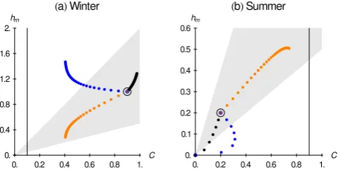
Fig. 6. Trajectories of the sea-ice state in the ice energy balance model with and without assimilation for one month of (a) constant winter forcing and (b) constant summer forcing. Positions for each day are marked by black points (trajectory without assimilation), blue points (trajectory with CMT assimilation), and orange points (trajectory with PMT assimilation). All trajectories start from the same initial conditions marked by the black circle. The target ice concentration is marked by a thin vertical line. The nudging param-eters are as in the AOGCM experiments. Mean ice thickness for a given concentration in the AOGCM is typically within the grey shaded area.
ume correction (CMT). The first test case is the assimilation of low sea-ice concentration under winter conditions with a downwelling shortwave radiation of 0 W m−2 and down-welling longwave radiation of 220 W m−2. The second test case is the assimilation of high sea-ice concentration un-der summer conditions with a downwelling shortwave radi-ation of 160 W m−2and downwelling longwave radiation of 300 W m−2.
Figure 6 shows the trajectories ofC andhm without as-similation, with CMT assimilation and with PMT assimila-tion for both test cases. Within the grey area that underlies the trajectories, the joint probability of occurrence forCand hmis higher than 0.1 %, as diagnosed from a long AOGCM run. In the following, we will call this the region of plausible ice states.
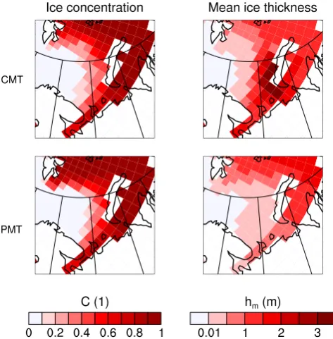
Fig. 7. Average March conditions 1990–1999 when assimilating ob-served sea-ice concentration in the AOGCM with the CMT method (top) and the PMT method (bottom). Ice concentration (left) is sim-ilar between CMT and PMT, and quite close to observations. How-ever, mean ice thickness (right) is much too high for CMT, and re-alistic for PMT.
For the summer test case (Fig. 6b), we let the trajectories start at low concentration and 0.2 m mean thickness. The tra-jectory without the relaxation term goes to an ice-free state within 6 days. When we nudge towards high concentration, the behaviour of PMT and CMT is again very different. The CMT trajectory loses ice volume; because for constant forc-ing the concentration loss is higher for thinner ice (see Eq. 6), concentration only initially increases, but soon the thermo-dynamic tendency outweighs the nudging tendency. Conse-quently, the CMT trajectory becomes ice-free within seven days, even though the data assimilation aims at increasing the ice concentration. Note that the melt is somewhat slower than without data assimilation, in accordance with the dependence of growth rate on concentration discussed in Appendix A3. On the other hand, the PMT trajectory gains ice volume, and stays inside the region of plausible ice states for the whole month.
In the AOGCM, an indication for the problematic be-haviour of the CMT method is found in the wintertime Bar-ents Sea (Fig. 7). During the 1990’s, the BarBar-ents Sea was mainly ice-free during winter, as derived from the satellite observations, whereas the model without assimilation is bi-ased towards ice-covered conditions. With assimilation, the ice concentration in this area decreases, but the decreased concentration leads to enhanced thermodynamic ice growth rates. As a result, there is unrealistically high ice volume
in conjunction with a reduced ice concentration if the CMT method is employed. Only when we apply PMT is this effect averted, as the nudging updates of ice volume compensate the excessive thermodynamic growth rates.
In summary, we have shown in this section that there are cases of practical relevance when the sea-ice growth rates as determined by the local surface energy balance necessitate adjustments of mean sea-ice thickness during the assimila-tion, as it is done in the CAT and PMT methods. This find-ing is consistent with results by Duli`ere and Fichefet (2007). Without these mean-thickness adjustments, as is the case for the CMT method, assimilation of ice concentration leads to implausible sea-ice states both in a conceptual IEBM and in the AOGCM.
6.2 Statistical aspects – model error covariances and weight matrices
We now take a different view on assimilation errors: instead of examining the sea-ice prognostic equations and how anal-ysis updates affect them, we examine the covariance structure of thickness and concentration errors in the AOGCM. There is a well-established theory that connects these so-called model background errors with the optimal analysis update; see, for instance, Bouttier and Courtier (1999) or Kalnay (2003). The analysis updates we apply are not optimal, but are derived from the simple nudging approach. Nevertheless, we can map our different choices for the analysis update to different model background errors that are implied under the assumption of optimality. If the implied model background errors are clearly unrealistic, we can argue that the assimila-tion method is prone to fail, since it is far from being opti-mal. We follow the notation of Bouttier and Courtier (1999) and briefly introduce the basic terminology in Sect. 6.2.1. We then apply the general terminology to our setup in Sect. 6.2.2, devising simplifications and a specialised notation. These simplifications and the specialised notation allow us to con-cisely discuss in Sect. 6.2.3 the relation between concentra-tion and mean thickness errors on the one hand and optimal analysis updates on the other hand.
6.2.1 Introduction of terminology
The state of a model that hasvvariables andp grid points is encoded in the state vectorx, a column vector withp·v entries. To obtain the analysisxa, i.e. our estimate of the true state xt, the model background xb is updated with a term that depends on the departure of the model state from the observationsy:
model state translate to analysis updates. It is called the gain, or weight matrix. If the weight matrix is chosen according to
Kopt=BHTHBHT+R
−1
, (16)
then the analysis in Eq. (15) is the best linear unbiased esti-mator of the true state (Bouttier and Courtier, 1999).
The optimal weight matrix Koptis related to the covari-ance matrices of background and observation errors B and R, defined by
B= h(b− ¯b) (b− ¯b)Ti R= h(o− ¯o) (o− ¯o)Ti. (17) The model background errorb=xb−xtdescribes the dis-crepancy between the modelled and the true state just before an analysis update. Therefore,b depends not only on the error of the model itself, but also on the applied analysis up-dates and the time interval between them. The observation erroro=y−Hxt expresses that the reported value of an observation is not a perfect image of reality, but is distorted due to instrumental and discretisation errors. B has dimen-sionspv×pv, and R has dimensionso×o.
6.2.2 Application to ice concentration and thickness
After introducing the general terminology, we now apply it to our setup. Because the simplicity of the setup allows for several algebraic simplifications, we can derive concise ex-pressions that are useful for understanding the interplay be-tween ice thickness and ice concentration errors. We order the state vectorxso that it starts with the entries for ice con-centrationCand ice mean thicknessh, followed by all other model variables:
x= C1, . . . , Cp, h1, . . . , hp, . . .T. (18) Sea-ice concentration is the only variable observed, and we are not interested in issues related to the interpolation from observation points to model points. Thus, we can assume a very simple form for the observation operator:
H= I 0. . ., (19)
with I denoting thep×pidentity matrix and 0 denoting the p×pzero matrix. Furthermore, the observation error covari-ance matrix R reduces to thep×pmatrix RCC.
We partition the background error covariance matrix B and the weight matrix K into submatrices of dimensionp×p that respectively describe the covariance between each pair of variables in the model, and the gains for each model vari-able resulting from the concentration observations:
B=
BCCBhC . . . BCh Bhh . . .
..
. ... . ..
K=
KCC KCh .. .
. (20)
Using Eqs. (18) to (20), the analysis update in Eq. (15) can be written as:
Ca ha .. . = Cb hb .. . + KCC KCh .. .
(Co−Cb) , (21)
and the optimal weight matrix (Eq. 16) reduces to a form that shows how the concentration and thickness background errors enter the optimal weight matrix:
Kopt=
BCC BCh .. .
BCC+RCC −1
. (22)
Equation (22) tells us how to obtain the optimal analysis update when we already know the correct statistics of the background and observation errors. Determining these error statistics is a difficult task within the data assimilation frame-work. Here, we are only interested in conceptual statements that can be derived from the error covariances, and so we es-timate them using simplifying assumptions. We assume that the observation error covariance RCC is spatially uncorre-lated and corresponds to a constant uncertainty of 10 %.
This value is a reasonable average error for concentration observation according to Tonboe and Nielsen (2010). We es-timate the background error covariances BCC and BChfrom the daily differences between concentration and thickness of two long, independent AOGCM runs. These background er-rors apply when the time interval between analysis updates is very large. For shorter time intervals between the analysis up-dates (one day for our setup), the absolute magnitude of the covariances is smaller, but we expect their spatial structure to be the same. For instance, in the central Arctic the sea-ice concentration is usually high, and thus we expect a low concentration background error variance, whereas we expect substantial background error covariance in areas that experi-ence a pronounced seasonal cycle of both thickness and con-centration.
From the model background error covariances we can also derive the correlation between concentration and thickness errors at the locationP:
corrP(C, h)=√ BCh(P ) BCC(P )Bhh(P )
. (23)
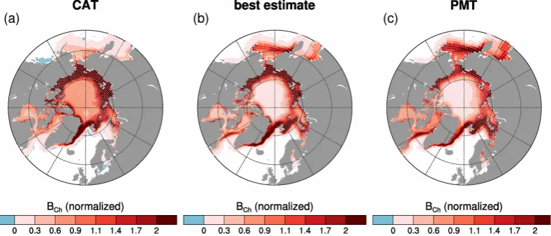
Fig. 8. Scaled diagonal elements of the background model error covariance matrices; (a) derived from Eq. (26) when analysis updates conserve actual thickness; (b) best estimate from a long free model run, and (c) derived from Eq. (27) for proportional mean-thickness analysis updates. The background error covariance implied by analysis updates that conserve mean thickness is zero everywhere. For an interpretation of the figure see main text.
6.2.3 Comparing nudging with optimal analysis updates
For the analysis updates of mean thickness, Eq. (22) defines the optimal weight matrix
KoptCh =BCh BCC+RCC
−1
. (24)
In our setup, we use weight matrices derived not from the optimality condition, but from an ad hoc nudging approach. Nevertheless, we can ask the following question: “Suppose the weight matrix KXCh used in method X is optimal, and we know the background error covariance for concentration BCC, what would be the implied background error covari-ance between concentration and thickness BXCh?” If BXCh is unrealistic, i.e. has substantial deviations from BCh, we can conclude that the weight matrix is far from being optimal and we reject an assimilation scheme that uses this weight matrix as being inconsistent.
For CMT, we do not update mean thickness at all, and so: KCMTCh =0Optimality⇐⇒ BCMTCh =0. (25) For CAT, we see from Eq. (10) that nudging weights vary in time and space, depending on the background actual thick-ness. We derive a time-averaged analysis update by diagnos-ing a diagonal matrix ht that contains the time average of actual ice thickness at each grid point over a long model run on the diagonal. With this, the average weight matrix and im-plied background error covariance are
KCATCh =KNht Optimality
⇐⇒ BCATCh =KNht(BCC+RCC) . (26) Finally, for PMT the weights are constant, because they are determined byh∗from Eq. (11). The weight matrix together
with its implied background error covariance matrix is given by
KPMTCh =KNh∗IOptimality⇐⇒ BChPMT=KNh∗(BCC+RCC). (27) The different background error covariances are compared in Fig. 8 by showing maps of their scaled diagonal elements. The absolute values of the covariances are not important, since they depend on the time interval between the analy-sis updates. However, the spatial distribution of high and low covariances has a large influence on the assimilation perfor-mance, as it determines the relative strengths of the optimal weights.
From Fig. 8b we see that background error covariances should be low in the perennial ice zone of the central Arc-tic, since there the concentration is always high, and low at the southern edge of the seasonal ice zone, since there the mean ice thickness is always low. In between, there is a re-gion where mean ice thickness and ice concentration co-vary strongly.
The CMT analysis updates imply a covariance structure that is very different from our best guess of the true covari-ance structure: it is zero everywhere. This implies a perfect representation of thickness forecasts in the model, which is a bad assumption, as we have seen in Sect. 6.1. Therefore, the CMT weight matrix is far from being optimal. Already from this simple analysis of background error covariance, one could have expected the poor assimilation performance seen in Sects. 4 and 5.
large there. On the other hand, the implied covariance is too low in the Bering Sea, the Labrador Sea, and the Barents Sea. One would expect the method to have difficulties assim-ilating observations there, since the analysis weights are too small.
Finally, the PMT updates shown in Fig. 8c imply a concentration–thickness covariance structure that is close to our best guess. There is a tendency to underestimate covari-ance in the Arctic shelf seas, and to overestimate it in the Hudson and Baffin Bays, but overall there is good agreement. We conclude that the comparison of the background error covariances implied by the chosen nudging weight matrices KCh corroborates the experimentally found differences be-tween the assimilation performance of the CMT, CAT, and PMT methods. Moreover, we think that the examination of implied background error covariance is a useful guide for designing weight matrices: only if the implied background error covariance looks plausible, can we expect a good per-formance of the assimilation method.
7 Summary and conclusion
We examine the performance of sea-ice data assimilation in a global climate model, using a simple Newtonian relax-ation approach. Analysis updates of sea-ice concentrrelax-ation are derived from the discrepancy between model and observa-tions, and analysis updates of sea-ice mean thickness (i.e. volume) are derived from the concentration updates. We in-vestigate three different approaches for the mean-thickness analysis updates. The first approach keeps the mean thick-ness constant during the analysis update (CMT). The sec-ond approach keeps the actual ice thickness constant (CAT). CMT and CAT have been suggested and used before in sea-ice data assimilation in an sea-ice–ocean model (Duli`ere and Fichefet, 2007), but we find that with our assimilation setup in an AOGCM they do not give satisfying results. Therefore, we introduce a third approach, which prescribes a fixed pro-portionality between concentration updates and mean thick-ness updates (PMT).
We establish four independent lines of evaluation by (i) comparing the simulated ice concentration and extent with observations, (ii) comparing simulated ice concentration and thickness with a reference simulation in an identical-twin ex-periment, (iii) considering conceptual arguments about the local ice energy balance, and (iv) considering the statistics of model background errors.
We find that PMT has much lower assimilation errors than the other two methods. For synthetic observation data de-rived from output of the same model (identical-twin study), PMT reduces the error of year-to-year changes in annual mean sea-ice extent to less than 0.1×10⁶km2, the error in annual mean sea-ice volume to 600 km3, the gridpoint-wise error in ice concentration to below 5 % throughout the year, and the gridpoint-wise error in mean ice thickness in the
Arc-tic Ocean to less than 30 cm. In contrast to these significant improvements, the impact of the assimilation on simulating other Arctic surface fields like sea-surface salinity and sur-face air temperature is only weak.
For the assimilation of observed sea-ice concentration be-tween 1979 and 2007, the PMT assimilation significantly re-duces differences between modelled and observed ice extent and concentration, with deviations becoming almost as low as in the identical-twin study. The monthly mean sea-ice vol-ume between 2005 and 2008 in the PMT assimilation is in good agreement with volume estimates derived from ICESat observations and the PIOMAS reanalysis, with deviations of less than 2000 km3.
The simplicity of the assimilation scheme allows us to ex-amine the assimilation errors with two conceptual tools: first, we apply the assimilation to a simple model of the local ice energy balance and conclude that the CMT method, where no adjustments to the mean thickness are made during the analysis update, causes unacceptable assimilation errors.
Second, we analyse the spatial structure of the background error covariance between concentration and thickness as im-plied by the nudging weight matrices of the different meth-ods and find that the spatial structure of the background er-ror is unrealistic for CMT, reasonable with some deficiencies for CAT, and realistic for PMT. These conceptual arguments support our experimental finding that the PMT method out-performs both CMT and CAT.
A drawback of our simple assimilation approach is that the model equations are not used in the analysis step, as they would be in four-dimensional variational data assimi-lation. Therefore, inconsistencies between our analysis up-dates and model physics are expected to occur, a property shared with several other data assimilation approaches. Our results show, however, that the parameters of our simple as-similation approach can be chosen such that we obtain im-provement of both ice concentration and ice thickness, and that we understand why some methods work better than oth-ers. Therefore we conclude that skillful sea-ice initialisation in an AOGCM is possible from ice-concentration data even with a simple Newtonian relaxation scheme, provided that we choose an appropriate functional relationship between concentration and mean-thickness analysis updates.
Appendix A
A simple radiative energy balance model for sea-ice mean thickness and concentration
A1 Derivation of the simple model
0 50 100 150 200 250 300 350 150
200 250 300 350
SW¯ HWm-2L
L
W¯
H
W
m
-2 L
W
S
Jan Mar
Apr
May Jun Jul
Aug
Sep
Oct
2 1
0
-0.5
-2
-3
-4
-5
g
i=0
T
i=0°
C
g w +
g
i=
0
g w =
0
Fig. 9. Contour plot of ice growth rates in cm day−1 for mean ice thicknesshm=1 m and ice concentrationC=0.7. On the x-axis is the downwelling shortwave radiation, on the y-x-axis the downwelling longwave radiation. The black dots correspond to the typical monthly-mean forcing in the Arctic according to Maykut and Untersteiner (1971). The blue and white lines mark the zero-crossing of the growth rates for open water and over ice, which are independent of the state of the ice. The thick black line is the zero-crossing of net growth rate, and depends on the state of the ice. At the dashed grey line, the ice surface temperature is at the melting point of 0◦C. The larger blue and red dots, labelled “W” and “S”, mark typical winter and summer conditions, for which the conditional probability distributions of growth rate in Fig. 10 are calculated.
equations for the ice concentrationCand mean ice thickness hm. These equations constitute a simple ice-energy-balance model (IEBM), which we use to analyse the ice growth rate for different atmospheric forcing regimes and to study how the analysis updates affect the thermodynamics of the ice.
The first simplification we make is to neglect sea-ice ad-vection. Since melting and freezing of ice are local pro-cesses, we can then solve the prognostic equations for mean thickness (Eq. 1) and concentration (Eq. 2) for each point in space separately. The thermodynamic source terms for sea-ice mean thicknessSh (Eq. 5) and sea-ice concentration
SC (Eq. 6) are determined by a balance of atmospheric and
oceanic heat fluxes at the sea-ice interfaces. An oceanic heat flux is established when sea-water warmer than the freezing temperature is brought into contact with the ice, while an at-mospheric heat flux occurs at the interface between atmo-sphere and sea ice or open water.
Since the dominant contribution to the sea-ice energy bal-ance in the Arctic is typically the surface radiation (Maykut and Untersteiner, 1971; Serreze et al., 2007), we neglect
Fig. 10. Conditional probability densities with which heat fluxes contributing to sea-ice growth occur for a given sea-ice concentra-tion. The occurrence probabilities were diagnosed from a long run of ECHAM5/MPI-OM for representative summer (a–c) and win-ter (d–f) conditions. Heat fluxes are given as equivalent ice growth rates (1 cm day−1=35 W m−2). Heat fluxes shown in (a and d) are between the ice and the atmosphere, and in (b and e) between the ice and the ocean. (c and f) show the net growth rates of the sea ice, which are equivalent to the sum of atmospheric and oceanic heat flux into the ice. The dashed green line is the dependence found in the simple radiative ice-energy balance model.
oceanic and turbulent atmospheric heat fluxes as a first ap-proximation and determine the ice growth rates from the ra-diative balance:
gw,i= − 1 ρL
(1−αw,i)SW↓+LW↓−σ Tw4,i
SW↓and LW↓are the downwelling shortwave and longwave
radiation at the surface, andαw,iis the albedo of open water or sea ice. In ECHAM5/MPI-OM, the surface temperature of open water in a partly ice-covered grid cell is always at a representative sea-water freezing temperatureTw= −1.9◦C, and the ice surface temperatureTiis calculated from the bal-ance of heat fluxes at the ice surface. We prescribe the at-mospheric downwelling radiation as an external forcing and determineSh andSC as a function of ice state and forcing.
Thereby, we can convert Eqs. (1) and (2) into a closed set of two coupled ordinary differential equations, which are forced by the time-dependent downwelling radiation at the surface. To obtain a closed set of equations using Eqs. (1), (2), (5) (6) and (A1), we need to determine how the growth ratesgw andgidepend on the forcing, i.e. downwelling longwave and shortwave radiation at the surface, and the state of the ice, i.e. concentration and mean thickness. These growth rates are directly proportional to the heat fluxesqw,ivia
gw,i= − 1
ρLqw,i. (A2)
The heat flux over open water in a partly ice-covered grid cell,qw, is easy to determine: the temperature of that open water is at the freezing point, so that the upwelling longwave radiation is constant. The heat flux over ice,qi, is more diffi-cult, since it depends on the ice surface temperatureTi. The ice surface temperature has to be determined from the bal-ance of the heat flux at the ice surfaceqiwith the conductive heat flux through the iceqc and a residual heat fluxqr that goes into surface melt:
qi=qc+qr. (A3)
The conductive heat flux through the ice is assumed to be proportional to the difference between the temperature at the top of the iceTi and the temperature at the bottom, which is always at the freezing temperatureTf. This is the so-called 0-layer model for ice growth suggested by Semtner (1976). The proportionality constant is the heat conductivity of icek divided by the actual ice thicknessht=hm/C. The conduc-tive heat flux as a function of ice surface temperature then is
qC(Ti)=
kC hm
(Ti−Tf) . (A4)
In our model, sea ice is assumed to melt at the freshwa-ter melting temperature Tm=0◦C at the top. When Ti<
Tm, there is no surface melt, qr=0, andTi can be derived fromqi=qc. With a linearisation of the black-body radia-tion aroundTm, we can solve forTiand obtain
Ti=
TfkC/ hm+(1−αi)SW↓+LW↓+3σ Tm4
kC/ hm+4σ T3 m
. (A5) The ice surface temperature cannot get larger thanTm in the model, because for Ti=Tm the residual heat flux
be-comes larger than zero,qr>0, and melts ice at the surface: qr
Ti=Tm=qi(Tm)−qc(Tm)=(1−αi)SW↓+LW↓ (A6) −σ Tm4−kC
hm(Tm−Tf) .
Inserting Eqs. (A4) and (A6) into Eq. (A3), we can write the net heat flux into the ice-covered part of the cell in a com-pact form:
qi=
kC
hm
(Ti−Tf)+δ(Ti−Tm) (−
kC
hm
(Tm−Tf)+(1−αi)SW↓ (A7) +LW↓−σ Tm4)
With this, we arrive at the following set of prognostic equations for the mean ice thicknesshmand the ice concen-trationC:
dhm
dt =giC+(1−C)gw (A8)
dC
dt =2(gw) gw h0
(1−C)+2(−Sh)
C 2hm
Sh, (A9)
where we can use Eqs. (5), (6), and Eqs. (A1–A7) to express each term on the right-hand side as a function only of the prognostic variableshmandCand the external forcings SW↓
and LW↓.
A2 Dependence of ice growth on atmospheric forcing
With Eq. (A1) we have an explicit expression for the ice growth rate, and we can study how it depends on the atmo-spheric forcing. If we are able to identify forcing regimes that differ among each other in the way the sea-ice thermodynam-ics reacts to changes in concentration, we will have important information for assessing the effects of the data assimilation on the prognostic equations.
Figure 9 shows the net growth rates derived from the IEBM for a sea-ice state of 1 m mean thickness and 70 % concentration. We can identify three different regimes, which are separated by the zero-growth contour over open water gw=0 and the zero-growth contour over icegi=0. Impor-tantly, the zero-growth contours are independent of the state of the ice and constitute the boundaries between three differ-ent forcing regimes.
small. This impliesgw< gi, and therefore the net growth rate increases with increasing concentration.
A3 Dependence of ice growth on ice concentration
To quantify the dependence of growth rate on ice con-centration, we select two representative forcing conditions: one for winter with SW↓=0 W m−2and LW↓=220 W m−2
(marked with a blue dot in Fig. 9), and one for summer with SW↓=160 W m−2and LW↓=300 W m−2(marked with a
red dot in Fig. 9). We calculate growth rates from the radia-tive budget of the IEBM described above, but there are two other contributions to the growth rate that we have neglected so far: the sensible and latent atmospheric heat flux, and the oceanic heat flux. Capturing these effects goes beyond the scope of the IEBM, but we can diagnose them from daily-mean fields of a long AOGCM run.
Figure 10 shows a synthesis of ice growth rates derived from the IEBM, and the occurrence of ice growth rates as di-agnosed from the AOGCM. During summer (Fig. 10a–c), the single curve obtained from the IEBM approximates the oc-currence of growth rates diagnosed from the AOGCM quite well, implying that oceanic contributions to ice melt as well as turbulent atmospheric heat fluxes are negligible. This is readily explained since the temperature of the near-surface atmosphere is close to the melting point, so that turbulent heat fluxes at the surface are small. At the same time, the ocean surface is warmed and becomes fresher, so that it gains buoyancy, and therefore convection is inhibited. Both in the IEBM and in the AOGCM, we observe a strong dependence of net ice growth rate on concentration: for the chosen at-mospheric summer forcing, ice melts at the rate of 1 cm per day for 100 % ice concentration, whereas it melts at a rate of more than 4 cm per day for very low ice concentration.
In winter, the IEBM is not a good approximation to the sea-ice thermodynamics in the AOGCM. As Fig. 10d shows, the curve determined from the radiative budget in the IEBM is actually at the lower boundary of the probability distri-bution of atmospheric growth rates. For open-water condi-tions, the IEBM predicts an atmospheric growth rate of 2 cm per day, whereas the most frequent value in the AOGCM is 5 cm per day, and even values of 8 cm per day occur quite often. The missing contribution comes from the turbulent at-mospheric heat flux, which can be very large over open water during winter. Only if the near-surface atmosphere stratifica-tion is very stable and near-surface winds are very weak, does the turbulent heat flux become so small that the AOGCM ex-hibits the dependence derived from the radiation budget in the IEBM.
Additionally, in winter the oceanic contribution to ice growth becomes large (Fig. 10e). The oceanic contribution can be due to horizontal advection of warm water under the ice, upwelling of warm water through Ekman suction, or en-trainment of warm water when the surface mixed layer deep-ens. The model shows high ocean-ice heat fluxes
predom-inantly close to the ice edge. The diagnostic we use does not differentiate between the processes, but we believe that the major contribution comes from entrainment of warm wa-ter from below during the deepening of the surface mixed layer. As Lemke (1987) pointed out, especially at the onset of freezing the convection can be vigorous enough to explain the magnitude of the ocean-ice heat flux that we see in the model.
For low ice concentration in winter, the ocean-ice heat flux strongly inhibits ice growth. The most frequent value of the ocean-ice heat flux, expressed as an equivalent melt rate, is 4 cm day, and even much larger values are possible (Fig. 10e). This compensates the large atmosphere–ice heat flux (Fig. 10d), so that the net growth rate in winter depends only weakly on the concentration (Fig. 10f). Nevertheless, since sea ice is closely coupled to the surface mixed layer below, it is the heat content of the coupled system of sea ice and surface mixed layer that is essential for the evolution of the ice. This heat content is determined by the atmospheric heat flux, and we therefore argue that the atmospheric growth rate in winter is more important than the net growth rate. The heat that goes from the mixed layer into the ice and inhibits ice growth cools the sea-water, so that ice formation is af-fected at a later time.
Acknowledgements. We thank Thorsten Mauritsen and Jai-son T. Ambadan for helpful discussions and two anonymous reviewers for thoughtful comments that helped improve the manuscript. This work was supported by the Max Planck Society for the Advancement of Science and the International Max Planck Research School on Earth System Modelling. All simulations were performed at the German Climate Computing Center (DKRZ) in Hamburg, Germany.
The service charges for this open access publication have been covered by the Max Planck Society.
Edited by: J. Schr¨oter
References
Blanchard-Wrigglesworth, E., Armour, K. C., Bitz, C. M., and DeWeaver, E.: Persistence and inherent predictability of Arctic sea ice in a GCM ensemble and observations, J. Climate, 24, 231–250, doi:10.1175/2010JCLI3775.1, 2011a.
Blanchard-Wrigglesworth, E., Bitz, C. M., and Holland, M. M.: Influence of initial conditions and climate forcing on pre-dicting Arctic sea ice, Geophys. Res. Lett., 38, L18503, doi:10.1029/2011GL048807, 2011b.
Bouttier, F. and Courtier, P.: Data assimilation concepts and meth-ods – training course lecture notes, from http://www.ecmwf.int (last access: 11 January 2013), 1999.