www.ocean-sci.net/6/887/2010/ doi:10.5194/os-6-887-2010
© Author(s) 2010. CC Attribution 3.0 License.
Ocean Science
Numerical simulations of spreading of the Persian Gulf outflow
into the Oman Sea
M. Ezam1, A. A. Bidokhti1,2, and A. H. Javid1
1Faculty of Marine Science and Technology, Science and Research Branch, Islamic Azad University, P.O. Box 14155-775, Tehran, Iran
2Institute of Geophysics, University of Tehran, P.O. Box 14155-6466, Tehran, Iran Received: 1 December 2009 – Published in Ocean Sci. Discuss.: 14 December 2009 Revised: 23 September 2010 – Accepted: 24 September 2010 – Published: 11 October 2010
Abstract. A three dimensional numerical model namely POM (Princeton Ocean Model) and observational data are used to study the Persian Gulf outflow structure and its spreading pathways during 1992. In the model, the monthly wind speed data were taken from ICOADS (Inter-national Comprehensive Ocean-Atmosphere Data Set) and the monthly SST (sea surface temperatures) were taken from AVHRR (Advanced Very High Resolution Radiometer) with the addition of monthly net shortwave radiations from NCEP (National Center for Environmental Prediction). The mean monthly precipitation rates from NCEP data and the calcu-lated evaporation rates are used to impose the surface salinity fluxes. At the open boundaries the temperature and salinity were prescribed from the mean monthly climatological val-ues from WOA05 (World Ocean Atlas 2005). Also the four major components of the tide were prescribed at the open boundaries. The results show that the outflow mainly orig-inates from two branches at different depths in the Persian Gulf. The permanent branch exists during the whole year deeper than 40m along the Gulf axis and originates from the inner parts of the Persian Gulf. The other seasonal branch forms in the vicinity of the shallow southern coasts due to high evaporation rates during winter. Near the Strait of Hor-muz the two branches join and form the main outflow source water. The results of simulations reveal that during the winter the outflow boundary current mainly detaches from the coast well before Ras Al Hamra Cape, however during summer the outflow seems to follow the coast even after this Cape. This is due to a higher density of the colder outflow that leads to more sinking near the coast in winter. Thus, the outflow moves to a deeper depth of about 500 m (for which
Correspondence to: M. Ezam
(ezam@srbiau.ac.ir)
some explanations are given) while the main part detaches and spreads at a depth of about 300 m. However in summer it all moves at a depth of about 200–250 m. During winter, the deeper, stronger and wider outflow is more affected by the steep topography, leading to separation from the coast. While during summer, the weaker and shallower outflow is less influenced by bottom topography and so continues along the boundary.
1 Introduction
The dynamics of dense fluids descending on an inclined boundary have been the subject of studies in oceanography. For example Jungclaus and Mellor (2000) investigated the Mediterranean outflow through the Strait of Gibraltar us-ing a three-dimensional numerical model (POM). They con-cluded that the outflow is controlled by pressure gradient, Coriolis force, entrainment and bottom friction. They spec-ulated that the combined effects of stratification, differen-tial entrainment, and routing by topography lead to the evo-lution of a two core structure in the bottom layer. The Mediterranean outflow after passing Cape St. Vincent be-comes hydro-dynamically unstable and lenses of saline water shed from the core and carry the outflow water characteristics into the Atlantic Ocean.
Pous et al. (2004) revealed short-term variability (about two weeks) of the Persian Gulf Outflow (PGO) by di-rect measurements using surface-drift buoys, hydrological and ADCP data. They attributed this variability to differ-ent mechanisms such as advection of the outflow, meander growth and eddy detachment from the outflow as it spreads into the Oman Sea, and diffusion of thermohaline properties of the outflow into the adjacent water masses. A number of individual hydrographic sections across the Gulf of Oman show that PGO moves along the southern boundary of the Gulf between 200 m to 400 m depth (Bower et al., 2000).
Matsuyama et al. (1998) investigated the vertical structure of the current and its time variations using ADCP measure-ment during December 1993–January 1994 in the Strait of Hormuz. They found that the diurnal tidal currents dominate over the semi-diurnal ones in the Strait of Hormuz. They also showed that for the diurnal tide, a tidal front forms during the spring tide but disappears during neap tide, thus the effective water exchange in the Strait occurs during neap tide. Density front formation depends on the strength of density stratifica-tion under the same tidal current, because the vertical mixing due to tidal current is suppressed by the strong density strat-ification.
Bidokhti and Ezam (2009) considered the vertical struc-tures of the PGO and surrounding waters in the Oman Sea using measurements from the ROPME (Regional Organiza-tion for the ProtecOrganiza-tion of the Marine Environment) expedi-tion of 1992 measurements (Reynolds, 1993). They argued that the outflow in the Oman Sea exhibits layered structures and attributed them to double diffusive convection as well as internal wave activities. They used a simple dynamical model based on conservation of potential vorticity and the assumption of geostrophic adjustment, to estimate the aver-age velocity and width of the outflow. They also tested some scenarios about salinity change and its effect on the volume transport and width of the outflow without including entrain-ment effects. They found (using this dynamical model) val-ues of 0.53 Sv and 0.42 Sv for PG outflow volume transport at the entrance to the Oman Sea during Feb. and May 1992 respectively. Johns et al. (2003) also estimated the outflow from the PG using direct ADCP measurements and found it
to be 0.15±0.03 Sv. This was based only on the measure-ments of one station near the southern coast of the Strait of Hormuz inside the Gulf.
In this paper, first a brief description of the three-dimensional numerical model POM is presented. Second, for the simulation of the PGO, the model preparation steps in-clude the modelling domain, data preparations and the initial and boundary conditions. Third, the model simulation results are compared with CTD measurements from the ROMPE ex-pedition in 1992. Finally, some characteristics of the PGO that are revealed from the model simulations such as spread-ing pathways, dynamical features in the Oman Sea and sea-sonal variations are presented.
2 The approach
2.1 The numerical model
The Princeton Ocean Model (e.g. Blumberg and Mellor, 1987; Mellor, 2003) is based on hydrostatic primitive equa-tions with Boussinesq approximation, terrain following co-ordinate (sigma coco-ordinate) system in the vertical and gen-eral orthogonal curvilinear system in the horizontal. The nu-merical grid employed for the spatial discretization is C-grid as presented by Mesinger and Arakawa (1976). The model uses the mode splitting technique which is the separation of the fast barotropic mode solved with high order explicit finite difference methods with external time step, from the slower baroclinic modes solved implicitly with internal time step. In the numerical solution the external and internal time steps are determined from stability condition (CFL, Courant-Friedrichs-Levy). For the external mode (barotropic mode), in the transport equations, the constraint of the time step is:
1tE≤ 1
Ct
1
δ x2+ 1
δ y2
−1/2
(1)
where: Ct=2(gH )1/2+Umax; Umax is the maximum ex-pected velocity in the domain (here 1 m s−1), andδx andδy
are horizontal grid spacings which are about 3.5 km in this case.
For typical coastal ocean condition, the ratio of internal to external time step is around 30–80 (Mellor, 2003). So we set it to 40.
54 54.5 55 55.5 56 56.5 57 57.5 58 58.5 59 59.5
22.5 23 23.5 24 24.5 25 25.5 26 26.5 27 -3500 -3000 -2500 -2000 -1500 -1000 -500 -120 -80 -60 -40 -20 0 Longitude Lat it u de
Ras Al Hamra Cape
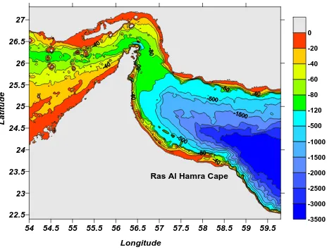
Fig. 1. The modelling domain and topography including east of
Persian Gulf and the Oman Sea.
when this background value increases to 10−4m2s−1and es-pecially to 10−3m2s−1the plume spatial structure changes dramatically. In addition, the effect of increasing the ver-tical mixing coefficient is especially noticeable in the up-shelf penetration of the plume and extension of its bulge. They also showed that if the background vertical diffusiv-ity increases to 10−4m2s−1more upstream intrusion is no-ticeable. Garvine (1999) suggested that, for high Richard-son number, holding the constant vertical mixing coefficients at a constant value of 10−4m2s−1and 10−3m2s−1instead of using the closure scheme, yields almost identical results. However, the effects of varying background vertical mixing coefficients are not investigated in this study.
Horizontal diffusions in the model are calculated from the Smogorinsky diffusivity formula as:
AM=C δx δy 1 2 " ∂u ∂x 2 + ∂v ∂y 2 + ∂w ∂z
2#1/2
(2) whereu,vandware velocity components in horizontal and vertical respectively, andC is a non-dimensional parameter and has been recommended to be in range between 0.1–0.2 (Mellor, 2003). Here it is chosen to be 0.2.
2.2 The model set up
The model domain is between 22.4–27.4◦N and 54–59.8◦E
that includes the eastern part of the Persian Gulf and the Oman Sea as indicated in Fig. 1. The bathymetry of the region was extracted from ETOP02 (Earth Topography 2 arc min), which contains global Earth topography includ-ing land with roughly 4 km resolution, and was interpolated to the grid size of the model. The horizontal grid resolutions are approximately 3.5 km and we employed 32 vertical lay-ers with non-uniform thickness in order to better represent the surface and bottom boundary layers.
‐350 ‐300 ‐250 ‐200 ‐150 ‐100 15 17 19 21 23 25 27 29 31 33 35
Jan Apr Jul Oct
Sh o rt Wa ve Rs d ia ti o n (W /m 2) Te m p e ra tu re (C ) Months SST
Air T
SWR (a) 0 0.02 0.04 0.06 0.08 0.1 0.12 0.14 0.16 0.18 0.2 20 25 30 35 40 45 50 55 60 65 70
Jan Apr Jul Oct
Ev ap . ‐ Pr e c. (m /m o n th ) Re la ti ve Hum idity (% ) Months RH EMP (b)
Fig. 2. Domain averaged time series of monthly: (a) Sea Surface
Temperature, air temperature and upward short wave radiation, (b) relative humidity and calculated evaporation minus precipitation in 1992.
Fig. 3. Typical mean monthly wind fields on the model domain in (a) February and (b) and May 1992.
The climatological annual mean of temperature and salin-ity was used as initial conditions for temperature and salinsalin-ity, and was extracted from WOA05 with 0.25◦×0.25◦
resolu-tion. The interpolation and extrapolation were performed to map these data on to the model grid in horizontal and verti-cal directions. The boundary conditions for the model and its setup configurations are given in Appendix A.
In order to calculate the mean monthly evaporation rate at the model grid points according to Eq. (A9), the mean monthly values of air temperature at 2 m above the sea surface (∼1.9◦×1.9◦) and mean monthly relative humidity
(2.5◦×2.5◦) in 1992, taken from NCEP data, were used.
The domain averaged time series of monthly SST, air tem-perature and upward short wave radiation are presented in Fig. 2a. In addition, the time series of the calculated monthly evaporation minus precipitation (EMP) and relative humidity are shown in Fig. 2b and typical mean monthly wind fields for Feb and May 1992 are shown in Fig. 3. It is interesting that the minimum value of EMP occurs in April when the surface wind is least.
3 Results and discussion
37 37.1 37.2 37.3 37.4 37.5 37.6
4 5 6 7 8 9 10
Sa lin ity (p su ) Years (a) 0 0.5 1 1.5 2
4 5 6 7 8 9 10
Ki n e ti c en er gy (m 2/s 2) x 10000 Years (b)
Fig. 4. Domain averaged time series of (a) the surface salinity and (b) the kinetic energy.
Fig. 5. Location of CTD stations during ROPME expedition (1992).
The lines show the cross-sections where model results are extracted.
Fig. 4. All time series have been plotted after taking the mov-ing average of 15 days intervals to filter the tidal and higher frequency changes. In this paper, the results of the last year of integrations are presented.
3.1 Comparison with observations
In this section, the model results are compared with some hydrographic measurements of the ROPME expedition in 1992. These data have been collected at two different times of the year and so the temporal variability of the outflow can be considered to some extent. A good review about the ROPME 1992 expedition and the data can be found in Reynolds (1993).
Locations of CTD measurements in the ROPME 1992 expedition during January–February (leg 1) and May–June (leg 6) are shown in Fig. 5. Typical profiles of CTD measure-ments during legs 1 and 6 for some stations and their almost corresponding points from model simulations are shown in Figs. 6 and 7. Generally, profiles from model simulations show relatively good agreement with observations. But some inconsistencies like the depth of the mixed layer (as seen in the 16 February station) or vertical salinity profile in deeper than 60 m in the 7 February station are also observed. These
36 37 38 39 40 41
-80 -60 -40 -20 0 Salinity (PSU) De pt h ( m )
20 21 22 23 24 25
-80 -60 -40 -20 0 Temperature (C) Staton 016 - Feb.
36 37 38 39
-100 -80 -60 -40 -20 0 Salinity (PSU) D ept h ( m )
20 21 22 23 24 25
-100 -80 -60 -40 -20 0 Temperature (C) Staton 007 - Feb.
35 35.5 36 36.5 37 37.5
-1000 -800 -600 -400 -200 0 Salinity (PSU) Dept h ( m )
5 10 15 20 25 30
-1000 -800 -600 -400 -200 0 Temperature (C) Staton 002 - Feb.
36 37 38 39 40 41
-80 -60 -40 -20 0 Salinity (psu) De p th (m)
20 21 22 23 24 25
-80 -60 -40 -20 0 Temperature (C)
36 37 38 39 40
-100 -80 -60 -40 -20 0 Salinity (psu) Dept h( m )
19 20 21 22
-100 -80 -60 -40 -20 0 Temperature (C)
35 36 37 38
-1000 -800 -600 -400 -200 0 Salinity (psu) D ept h( m )
5 10 15 20 25
-1000 -800 -600 -400 -200 0 Temperature (C)
Fig. 6. Typical salinity- temperature profiles during February from
CTD measurements (top) and model simualtions (bottom). Loca-tions are shown in Fig. 5.
36 37 38 39 40
-80 -60 -40 -20 0 Salinity (PSU) De pt h ( m )
20 22 24 26 28
-80 -60 -40 -20 0 Temperature (C)
Staton 016 - May
36 37 38 39
-100 -80 -60 -40 -20 0 Salinity (PSU) D ept h (m )
20 22 24 26 28 30
-100 -80 -60 -40 -20 0 Temperature (C)
Staton 007 - May
35.5 36 36.5 37 37.5
-1000 -800 -600 -400 -200 0 Salinity (PSU) D ept h (m )
5 10 15 20 25 30 35
-1000 -800 -600 -400 -200 0 Temperature (C)
Staton 002 - May
36 37 38 39 40
-80 -60 -40 -20 0 Salinity (psu) D e pt h( m )
20 22 24 26 28
-80 -60 -40 -20 0 Temperature (C)
36 37 38 39
-100 -80 -60 -40 -20 0 Salinity (psu) D e pt h( m )
20 25 30
-100 -80 -60 -40 -20 0 Temperature (C)
35 36 37 38
-1000 -800 -600 -400 -200 0 Salinity (psu) D e pt h( m )
10 20 30 40
-1000 -800 -600 -400 -200 0 Temperature (C)
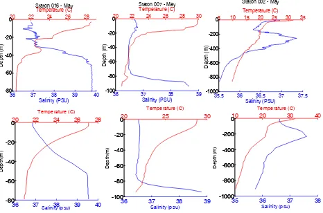
Fig. 7. Typical salinity- temperature profiles during May from CTD
measurements (top) and model simualtions (bottom). Locations are shown in Fig. 5.
can be due to the fact that we present monthly mean pro-files of model simulations while the CTD measurements are collected in a short period of time so that short time variabil-ities are included in these measurements due to tidal mixing, instabilities, daily cooling and heating. Also, we have used coarse resolution monthly mean climatological temperature and salinity as representative of inflow characterictics at the open boundaries, and thus the interpolation errors and time varibility must be considered.
3.2 The outflow characteristics
In order to investigate the PGO characteristics at the entrance to the Oman Sea, we focus on the transect IJ (see Fig. 5). Defining the isohaline of the PGO source boundary (SO)as an indicator to distinguish it from the surrounding water by:
38.5 38.7 38.9 39.1 39.3 39.5 39.7 39.9 18 20 22 24 26 28
4 5 6 7 8 9 10
Sa lin ity (p su ) Te m p e ra tu re (c ) Years T S (a) 0.1 0.2 0.3 0.4 0.5 0.6 0.7 25.5 26 26.5 27 27.5 28 28.5
4 5 6 7 8 9 10
Vo lu m e fl u x (S v) Si gm a ‐ T (k g /m 3) Years Sigma‐T Vol. Flux (b) 38 38.5 39 39.5 40 18 20 22 24 26 28
Jan Apr Jul Oct
Sa li n it y (p su ) Te m p e ra tu re (C) Months T S (C) 0.0 0.1 0.2 0.3 0.4 0.5 0.6 0.7 24.5 25.0 25.5 26.0 26.5 27.0 27.5 28.0 28.5
Jan Apr Jul Oct
Vo lu m e fl u x (S v) Si gm a ‐ T (k g /m 3) Months Sigma‐T Vol. Flux (d)
Fig. 8. Time series of (a) the mean PG outflow temperature, salinity,
(b) volume flux andσ-T. (c) The monthly mean for the last year
of integrations of the outflow temperature, salinity, (d) volume flux andσ-T, at transect IJ (see Fig. 4).
whereSmax is the maximum of the observed salinity, and
Ssurris the area averaged salinity on transect IJ, we can esti-mate the mean outflow temperature, salinity,σ-T. The vol-ume transports at this transect are calculated by integrating the southward component of velocities corresponding to the outflow source water. Figure 8a and b shows time series of outflow temperature, salinity, σ-T and volume transport at transect IJ. The monthly mean values of outflow characteris-tics were calculated for the last year of integrations as shown in Fig. 8c and d.
The time series show that the PG outflow has an annual variability in temperature between 19.7 and 26.8◦C in March and August respectively with a mean annual value of about 24◦C. Its salinity is relatively constant and is about 39.3 psu with an annual change of about 0.2 psu. The outflowσ-T
varies between its minimum (26 kg m−3) in August to its maximum values (28.2 kg m−3)in March with a mean an-nual of about 26.8 kg m−3.
The maximum volume transport of the PG outflow oc-curs during February–March (about 0.57 Sv) and it reaches its minimum value in November (about 0.23 Sv) with an an-nual mean of about 0.35 Sv at the transect IJ. The simula-tion results are consistent with finding of Bidokhti and Ezam (2009) but are greater than the estimates of Johns et al. (2003) with an annual mean of 0.2–0.25 Sv for the PG outflow trans-port. It may be due to the fact that we estimated the PG volume transport at the entrance to the Oman Sea where di-lution could have increased the volume transport. Bower et al. (2000) have estimated the dilution of the Persian Gulf wa-ter to the Oman Sea by factor of∼4.
Fig. 9. T-S diagrams of water in the Oman Sea in the box shown in
Fig. 5 for March (left) and August (right).
Typical T-S diagrams of the water masses in the Oman Sea for March and August are presented in Fig. 9, indicating that the salinity of the outflow source water is nearly the same for both months (between 39–40 psu). Also the temperature of the outflow source water in March is almost constant and is about 19◦C, but during August, its temperature varies be-tween 22 and 25◦C (that may be related to the existence of the outflow at different depths along its path). In the Oman Sea, the product waters are indicated by water masses with temperature of about 20◦C for March and a little higher tem-perature of about 22◦C for August. The salinity of product water however, is nearly the same and is about 37.5 psu for both months. Accordingly, the meanσ-T of product water is about 26.5 and 26 kg m−3in March and August respectively. It is also clear that the outflow temperature increases a lit-tle from its source in the Persian Gulf to its equilibrated po-sition in the Oman Sea during March, while the temperature reductions of about 4◦C is observed in outflow during Au-gust.
3.3 The outflow spreading pathway
Here, the outflow spreading pathways is investigated at some cross-sections from the inner Persian Gulf to the Oman Sea where it reaches its equilibrium depth during March and Au-gust, which are the months when the outflow has its maxi-mum and minimaxi-mum initial densities (see Fig. 8d). Then hor-izontal fields are presented to show the spreading pathways. All transects and horizontal fields are plotted after averaging every month to filter the tidal and high frequency changes.
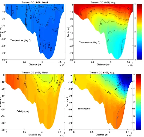
The transects of temperature and salinity in the Persian Gulf (transect CD, Fig. 10) show during March that the tem-perature is nearly constant and varies from 19–20◦C from
Fig. 10. Cross-section of the mean temperature and salinity along
CD path, shown in Fig. 5 obtained from model simulation during March (left) and August (right).
Generally, the simulations indicate that the PGO origi-nates from two branches; one permanent branch exists dur-ing almost the whole year in deeper than 40 m and may form from inner parts of the Persian Gulf. A seasonal branch which forms in the winter months originates from the shallow southern parts. The seasonal branch due to its higher density relative to surrounding water sinks to the deeper zone and joins the permanent branch. Finally, these two branches form the PGO in the bottom of the Gulf in the southern deep part of the Strait of Hormuz (transect IJ). This may have some implications for the outflow depth in the Oman Sea (see be-low).
Figure 11 shows the monthly mean temperature, salinity andσ-T along transects IJ in March and August. In March, the temperature shows a nearly homogenous structure as be-fore in transect CD, and the source of the outflow is indi-cated by the water mass with salinity above∼39 psu and a temperature of∼19.5◦C. In August, the vertical tempera-ture differences up to 10◦C are observed, with a strong ther-mocline near the surface. The outflow is indicated by salin-ity above∼39 psu, while its temperature varies between 24 and 26◦C. Hence, the mean outflowσ-T varies from about 28.1 kg m−3 during March to about 26 kg m−3 during Au-gust, which mainly results from outflow temperature varia-tions of more than about 6◦C.
In the eastern half of the transects, salinities are nearly the same from the surface down to the depth of 60 m for both months and are about 36.5 psu. But, in the western half of the transects, salinity is higher in August, especially above the depth of 40 m. This may be due to the advection of saline
Fig. 11. Cross-section of the mean temperature, salinity andσ
-T along IJ path, shown in Fig. 5 obtained from model simulation during March (left) and August (right).
water by eddies and also to the lower density stratification during August that lead to higher mixing with surrounding waters. As shown in σ-T transects, during March (win-ter months) a two layer density regime is observed, namely an upper layer with σ-T of about 26 kg m−3 and a lower layer withσ-T values larger than 28.5 kg m−3. In these tran-sects, pycnostads (characteristic of strong baroclinic ocean currents) are observed.
During August, (summer) a three layer stratification is ob-served, namely an upper low density layer withσ-T of about 23 kg m−3, an intermediate layer with about 25.5 kg m−3and a lower layer with about 27 kg m−3. It can be concluded from these values that during March higher density differences be-tween benthic layer and upper layer (about 2.5 kg m−3)leads to higher stratification. Therefore the entrainment and mix-ing between the outflow and upper layer decreases in com-parison with August when the density difference is weaker in the water column (about 1.5 kg m−3).
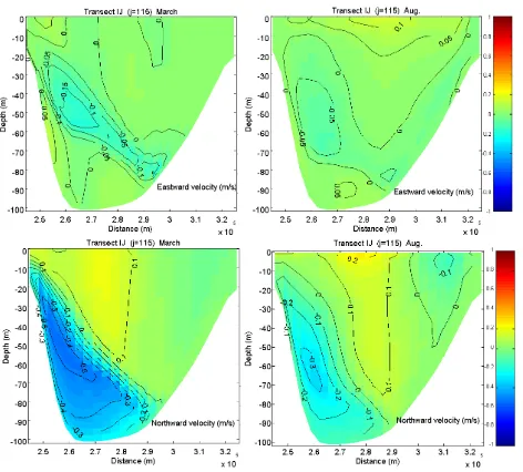
Fig. 12. Cross-section of the mean velocity components along the IJ
path shown in Fig. 5, obtained from model simulation during March (left) and August (right).
depths of 30–70 m with more than 0.5 ms−1 in March, and at depths of 50–70 m with a velocity of about 0.3 ms−1 in August. The direction of the outflow at these depths is mainly southward. This may make the outflow supercritical (Froude number larger than 1) only for winter as it enters the Oman Sea. The westward component of the flow can be due to thermal wind effects that cause the flow to turn right with height in the Northern Hemisphere.
The T and S characteristics of the outflow along tran-sect MN are shown in Fig. 13. The main outflow branch is identified in salinity and temperature transects, as saltier and warmer water mass relative to the surrounding water, banks against western coast. In addition, patches with higher salinity and warmer water are also observed that can be the result of instability of the outflow plume and eddy activi-ties. Here, the outflow salinity is nearly the same for both months∼38 psu, but its temperature is about 20◦C and 24◦C for March and August respectively. It indicates an increase (small decrease) of outflow temperature from its source in the Persian Gulf to the Oman Sea where it reaches the equi-librium depth during March (August).
The denser outflow source water in March, and also lesser entrainment and mixing in comparison with August, lead to outflow intrusion at larger equilibrium depths. Thus, the equilibrated outflow is observed with mean depths of about 200 m and 500 m during August and March respectively. The σ-T transects (not shown) also confirm that the out-flow has reached its equilibrium levels. Figure 9 of Bidokhti and Ezam (2009) based on measurements of ROMPE 1992 also shows that the outflow higher density extends well into deeper part of the Oman Sea in winter in comparison with that of summer (for further discussion see below).
Fig. 13. Cross-section of the mean temperature and salinity along
the MN path, shown in Fig. 5 obtained from model simulation dur-ing March (left) and August (right).
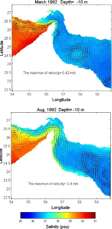
The horizontal sections of salinity with overlaid velocity field at depth of 10 m are shown in Fig. 14 for March and August. The figure shows the saltier Persian Gulf water dur-ing March in the southern part of the Gulf sinks at the Strait of Hormuz and is not observed at the depth of 10 m after the Strait. While in August at least part of the outflow moves along the coast of the Oman that indicates it is less dense than that of March period.
In the Oman Sea in March, a dominant cyclonic eddy is observed between 57.5–58.5◦E and 24–25◦N with mean ve-locity of about 0.3 ms−1. Interestingly, in August nearly at the same place (58–59◦E and 24–25◦N), the dominant eddy is an anti-cyclonic one with mean velocity of about 0.32 ms−1. It appears that the near surface eddy might be generated by the outflow in winter in which it intrudes deeper and the surface winds in Oman Sea are weaker, while in summer the outflow is not as deep and the surface winds in Monsoon time is stronger which may create the anti-cyclonic eddy.
Fig. 14. The mean monthly of horizontal salinity and velocity fields
at depth 10 m for March (up) and August (down).
part finds its equilibrium depth and spreads in the vicinity of the coastal boundaries at shallower depths (see Fig. 15). It seems interesting that the dominant circulation in the Oman Sea in August becomes cyclonic at this depth (Fig. 15), while the surface cyclonic eddy observed in winter still exists at 80 m. Hence the outflow at the depth of 80 m appears to con-trol the circulations in both seasons at this depth.
The maximum outflow velocities occur where the bottom slope suddenly increases. These velocities are 0.69 ms−1and 0.35 ms−1for March and August respectively and are nearly consistent with Bower et al. (2000), who showed the out-flow reaches its maximum speed in winter (0.55 ms−1)and its minimum in summer (0.4 ms−1).
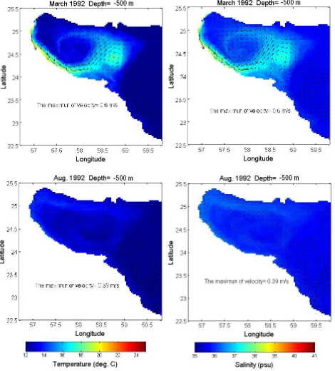
Figures 16 and 17 show the horizontal fields of the tem-perature, salinity and the overlaid velocities at depths 200 m and 500 m, which are related to the equilibrium depths of the outflow during August and March respectively. The lower source density of the outflow during August causes the ap-pearance of the outflow in the shallower zone relative to that
Fig. 15. Horizontal mean fields of temperature (left) and salinity
(right) in extended view of the Strait of Hormuz and Oman Sea at depth 80 m during March and August.
Fig. 16. Horizontal mean fields of temperature and salinity at depth
Fig. 17. Horizontal mean fields of temperature and salinity at depth
500 m for March and August.
of March. Hence, in August the outflow is more evident at the depth of 200 m and propagates as a narrow boundary cur-rent in vicinity of southern and western coasts, disappear-ing downstream of the the Ras Al Hamra Cape (located at 58.5◦E and 23.8◦N).
As a whole, it could be concluded that during August, the low outflow density and volume flux only create a weak cir-culation at the depth of the outflow with no substantial effects in the deeper parts. However in March the outflow effect is observed deeper with a marked cyclonic eddy (also seen up to the surface) that appears to be generated by the outflow as it detaches from the bottom of the southern border and spreads into the central part of the Oman Sea. This eddy as well as a smaller anti-cyclonic one are formed further east (Fig. 17) at the depth of the outflow in winter (about 500m). The smaller anti-cyclonic eddy (Peddy, Persian Gulf eddy) contains more outflow characteristics. Senjyu el al. (1998) used field measurements of January 1994 to study the Peddy formation and suggested that it is related to the intermittency of outflow movement through the Strait of Hormuz. They found the depth of the eddy is in the range of 250–400 m (see Fig. 18).
Several other eddy generation mechanisms have been pre-sented in the literature. For example d’Asaro (1988) sug-gested that a coastal trapped boundary current may gain anti-cyclonic vorticity as a result of viscous stress in the boundary layer when it arrives at a cape or canyon. D’Asaro used this theory to explain the permanent existence of an anticyclone
Fig. 18. Locations of CTD measurements during January 1994
(Senjyu et al., 1998) and the corresponding salinity transect.
in the Arctic Ocean. He also speculated that Mediterranean eddies (Meddies) could be generated by the same mechanism as the Mediterranean outflow separates from the continental slope. Bower et al. (1997) from numerous Lagrangian obser-vations and implementation of the d’Asaro model explained the production of Meddies at Cape St. Vincent.
Jungclaus (1999) investigated the evolution of buoyancy driven intermediate flow along an idealized continental slope using a three-dimensional numerical ocean model (POM). He showed that the intruding outflow interacts with overlay-ing water and vortex compression and stretchoverlay-ing takes place. He speculated that the lateral intrusion of the plume into the ambient water column compresses the water above and be-low and thus anti-cyclonic vorticity is introduced in order to conserve the potential vorticity.
We also performed the simulation without including the tide. The results show that separation of the outflow from lateral boundary occurs as before. But the outflow spreads as an “S” shape meander, and the mentioned Peddy may not form (however, in the absence of tide the salinity and tem-perature of the outflow change a little because of less mixing induced by tide especially in the Strait of Hormuz). Hence, these results agree more with Senjyu et al. (1998).
Stern (1980) showed that for a coastal gravity current with zero potential vorticity assumption, if the current width far upstream of the nose is less than a critical fraction (0.42) of the Rossby radius of deformation (based on the current depth far upstream), then the nose of the current will propa-gate along the coast as a bore and the form of the nose may be steady if the friction is able to dissipate sufficient kinetic en-ergy. If the upstream current is wider than this critical value the flow may be blocked and deflected perpendicular to the coast causing separation.
We implemented the Stern theory (however the outflow vorticity may not be zero) to study the behaviour of the outflow near the Ras al Hamra Cape. Extracting the out-flow characteristics at a place before the Cape yields: h∼
500, 200 m (outflow depth); g0∼0.015, 0.012 ms−2 (re-duced gravity), w∼40, 10 km (outflow width) and f ∼
Fig. 19. Time-depth rate of changes of temperature (a) and salinity
(b), at a station off the coast of the Oman Sea located at 57◦E and
24.7◦N. The horizontal axis is scaled from January to December.
deformation (pg0h/f), are approximately equal to 46 and
24 km for March and August respectively, that lead to crit-ical current widths of order of 19 km for March and 11 km for August. Comparing these values with outflow widths, it could be concluded that during March the outflow should de-tach from the coast and propagate normal to the coast, while during August it could continue its propagation along the coastal boundary (as seen in Figs. 16 and 17).
An additional explanation for the separation and Peddy formation is that during March, as the PG outflow moves to deeper zone of the Oman Sea, encountering the steep to-pography near the Ras al Hamra Cape (as seen in Fig. 1), the outflow thickness increases (due to stretching processes) and so the compression of water column above and below it take places. Therefore, due to conservation of the potential vorticity an anti-cyclonic circulation may be introduced (as speculated by Jungclaus, 1999).
The time-depth rate of changes in temperature and salinity for the last integration year at a station off the Oman Coast at (57◦E and 24.7◦N) near the path of the outflow are shown in Fig. 19. It is interesting that the mean depth of the outflow is at about 200–300 m in the second half of spring, summer and autumn, but as winter begins it sinks to a depth of 400– 600 m until late April and after which it moves to upper depth again. This winter sinking of the outflow appears to be due
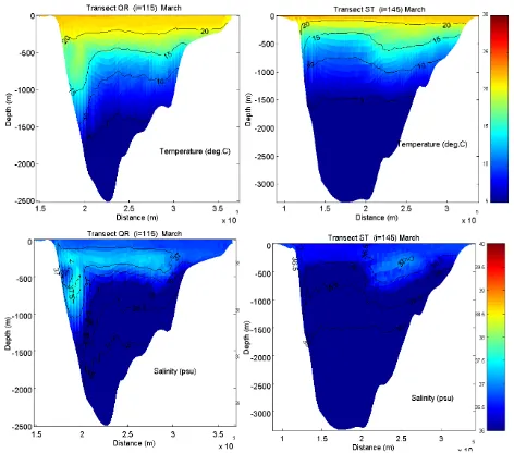
Fig. 20. The mean monthly temperature and salinity along QR and
ST cross sections (see Fig. 5) in March.
to colder temperature of the outflow source water and has not been observed by field studies which are very rare for this area. In some previous literatures (e.g. Senjyu et al., 1998; Bower et al., 2000; Pous et al., 2004) the mean depth of the outflow spreading in the Oman Sea has been found to be at about 250–400 m. The results of this simulation are more or less consistent with the measurements of Senjyu et al. (1998) (Fig. 18), which have been made during January 1994, and the measurements of the Pous et al. (2004), during October and early November 1999. However, more direct measure-ments are required to verify deeper outflow in late winter in the southern part of the Oman Sea.
‐0.4
‐0.2 0 0.2 0.4 0.6 0.8 1 1.2
0 10 20 30
Vo
lu
m
e
fl
u
x
(S
v)
Days
March Aug.
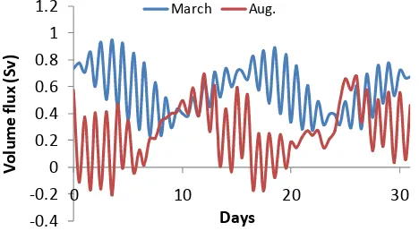
Fig. 21. The short-time variations of the outflow transports during
March and August. The data are plotted in half day intervals.
model. Another factor is that some down-welling process in winter may at least sink part of the outflow near the southern boundary as Spall (2008) has shown that such process may results from surface buoyancy loss. Or as the denser out-flow in winter can be supercritical just as it enters the Oman Sea, this leads to deepening of its initial path (Afanasyev and Peltier, 2001). In winter, we also showed above that the source water from the PG has an extra branch (cold and salty one along the southern coast, Fig. 10) just before exiting the PG and this could enhance the density of the outflow com-pared to that of other times when there is mainly the axial deeper branch. Therefore there are a variety of effects that may lead to this winter deepening of part of the outflow near the Oman coast in its initial stage that are required to be fur-ther investigated.
3.4 Effects of tide
In this section, the interactions of the PGO and the tidal front in the Strait of Hormuz are investigated. This interaction causes the intermittency of the outflow into the Oman Sea. We compare the short time variations of the outflow volume fluxes during March and August at the transect IJ, which are related to the maximum and minimum vertical stratifications respectively. The time series of the outflow discharges during March and August are shown in Fig. 21, which are plotted in half day intervals. The series show that in March, the dis-charges of the outflow oscillates between 0.9 Sv and 0.23 Sv during the tidal cycle, while these values are between about 0.69 Sv and−0.15 Sv for Aug (only based on the flow of source water with salinity defined by Eq. (13)). These values suggested that during March the outflow is always moving into the Oman Sea, however, its transport varies due to in-teraction with tide. But during August, in addition to the decrease in the maximum discharge of the outflow due to variations in source water characteristics, it seems that there are occasions when the movement of the outflow to the Oman Sea is suspended or somehow reversed by tide.
Fig. 22. The snapshots ofσ-T and velocity fields in the minimum
and maximum outflow transports during March and August.
These could be related to stronger stratification during March (winter) that leads to less mixing and hence higher outflow density relative to August (summer) as seen in Fig. 11. As a result the outflow movement persists during March, while weaker stratification in August leads to more tidal mixing and hence to occasional outflow suspension. The snapshots ofσ-T and velocity fields related to maxi-mum and minimaxi-mum of outflow transports during March and August are shown in Fig. 22 which also indicates these inter-active variations.
4 Conclusions
A numerical study of the PG outflow including its impacts on the physical properties of the Oman Sea has been carried out using a three-dimensional model, namely the Princeton Ocean Model that has been used widely for estuarine, coastal waters and open-ocean application modelling. The simula-tion was performed for the year 1992 since direct CTD mea-surements are available in the region at two different times (early winter and early summer) from the 1992 ROPME ex-pedition.
27◦C. This leads to the variations in the outflow density
of order of 2 kg m−3 during the year. The maximum and minimum densities of the outflow occur during late winter (March) and midsummer (August) respectively. The highest density of the outflow source water causes it to penetrate to the deeper depths in the Oman Sea during March.
During summer the outflow has a lower source density, hence it spreads into the shallower depths near the coastal boundaries. During March (winter) the outflow with higher density spreads into the deeper parts and separate from the lateral boundary as it approaches the Ras al Hamra Cape, and the larger width of the outflow, steep topography and tidal os-cillations appear to generate the Peddies. The inconsistency between the predicted depth of part of the outflow in winter and the limited observational data are indicated in terms of the effects of the possible limitation of sigma coordinate over steep topography, the resolution of the western boundary data for temperature and salinity, double diffusion, surface strong winter buoyancy loss or the flow being supercritical as it en-ters the Oman sea. Examining these is required for further study of such behaviour.
As a whole, we find that the seasonal variations of the outflow source water characteristics lead to different outflow pathways in the Oman Sea. The outflow is affected by differ-ent mechanisms in the Strait of Hormuz and the Oman Sea such as vertical mixing due to interaction by tide that leads to intermittency in outflow into the Oman Sea. The short time variability of the outflow and other dynamical processes such as barotropic and baroclinic instabilities can lead to the outflow intermittency and as a result eddy generation in the Oman Sea which is not considered in the present work.
We also examined the role of tidal mixing on the initial density of the outflow source water. The results indicated that the mean salinity of the outflow source water could reach to more than 40.2 psu (as opposed to 39.3 psu) when tide is not included in the simulations (it is not shown here). It shows that tidal mixing has a strong effect on the initial density of the outflow source water at the Strait of Hormuz.
Finally, it is necessary to say that we used the coarse res-olution monthly mean climatological data as representative of salinity and temperature of the inflows to the model do-main. It is believed that the more accurate prescriptions of
T andSfrom direct measurements at the western boundary, or eliminating the western open boundary by extending the modelling area to the entire Persian Gulf and the Oman Sea, will improve the model simulation results.
Appendix A
Boundary conditions
A1 Open boundary conditions (OBCs)
For the external mode, the normal barotropic velocities at the open boundaries are considered by a type of radiation bound-ary condition (e.g. Flather, 1976; Korres and Lascaratos, 2003; Mellor, 2003) of the following form:
H U±ceη=0 (A1)
whereH is the water depth at corresponding grid,U is the normal barotropic velocity, ce is the external mode phase speed and is equal to√gH andηis the sea surface eleva-tion at corresponding grid.
The amplitudes and phase speeds of the four major tidal constituents (M2, S2, O1 and K1) are prescribed at the open boundaries from the Admiralty Tide Table and assumed as constant along the boundaries. The data are relevant to Kish Island at the western and Konarak port at the eastern bound-aries in vicinity of the Iranian coast. However, these lead to less than 10% errors in prescriptions of each tidal constituent (amplitudes and phases) near the Strait of Hormuz, where the interaction between density front and tidal front occurs, and thus seem to be appropriate for the aim of this study.
For the surface elevation at the boundaries, a zero gradient condition of the following form is adopted:
∂η
∂n=0 (A2)
For the internal mode, the baroclinic normal velocities at the open boundaries are calculated by adapting the Sommerfeld radiation condition:
∂ui
∂t +ci ∂ui
∂n =0 (A3)
where,ui is the normal baroclinic velocity, nis a direction
perpendicular to the open boundary andciis the phase speed of internal mode propagation and is calculated using Orlanski (1976) scheme.
In both barotropic and baroclinic modes, the component of the velocities parallel to the open boundaries are assumed to be zero.
For the temperature and salinity at the open boundaries, whenever the normal velocity is directed outwards from the model domain, an upstream advection scheme of the follow-ing form is adopted (e.g. Kantha and Klayson, 2000; Mellor, 2003):
∂T ∂t +ui
∂T ∂n =0,
∂S ∂t +ui
∂S
∂n=0 (A4)
(0.25◦×0.25◦). These data are interpolated and extrapolated
at the open (eastern and western) boundaries to represent the thermohaline characteristics of the inflow water into the modeling area.
A2 Surface boundary conditions
The momentum boundary condition at the surface is set to:
−KM ∂U∂z, ∂V∂zz=0=
τx, τy
z=0
ρw
(A5) where τx, τyz=0=ρaCD|U10|(U10, V10)
whereKMis the vertical kinematic eddy viscosity, (τx,τy)is
the directional wind stress at the sea surface,ρwandρaare the density of water and air respectively,|U10|is the mag-nitude of the wind speed at 10 m level above the sea surface andCD is the wind speed dependent drag coefficient and is calculated according to Geernaert et al. (1986) as follows:
CD=10−3(0.43+0.097|U10|) (A6) In the model, the monthly mean values of wind speed com-ponents over the domain are taken from ICOADS in 1992 (1◦×1◦resolution) and are interpolated onto the model gird.
The sea surface temperature boundary condition is:
T|z=0=TS (A7)
where TS is the SST prescribed from AVHRR data with 0.04◦×0.04◦resolution. The monthly mean values of SST in 1992 are mapped on the model grid after interpolation.
In addition, the monthly mean net shortwave radiation is applied at the sea surface and is taken from NCEP with approximately 1.9◦×1.9◦ resolution interpolated onto the model grid points.
The sea surface salinity boundary condition is set to:
−KH ∂S∂zz=0=QS= −
SS
ρW
◦
E− ◦
P
(A8) whereKHis the vertical eddy diffusivity,QSis the salt flux at the surface, SS is the model surface salinity,
◦
E andP◦
are evaporation rate and precipitation rate respectively. In Eq. (A8) the mean monthly precipitation rates in 1992 are taken from NCEP data (∼1.9◦×1.9◦) and are interpolated
onto the model grid points, and the evaporation rates are cal-culated according to the classical bulk aerodynamic formula (Korres and Lascaratos, 2003) by:
◦
E=0.622CE|U10|(eSAT(TS)−R eSAT(TA))
ρA
PA
(A9) whereCE is the turbulent exchange coefficient and is cal-culated using a formula given in Kondo (1975). eSAT is the atmospheric saturation vapor pressure and is computed through a polynomial approximation as a function of tem-perature (Lowe, 1977), PA is the atmospheric pressure, R
is the relative humidity,TA is the air temperature in Kelvin at 2 m above the sea surface, ρA is the density of moist air and is computed as a function of air temperature and relative humidity.
Acknowledgements. We would like to thank the ocean modelling
department of Princeton University for making the code available online, and the anonymous referees of the OS journal because of their contributions and constructive comments concerning this paper. In addition, we appreciate the OS editorial board for their efforts during review process, especially J. Johnson for English improvement of the paper.
Edited by: J. Johnson
References
Afanasyev, Ya. D. and Peltier, W. R.: On breaking internal waves over the sill in Knight Inlet, Proc. R. Soc. Lond., 457, 2799– 2825, doi:10.1098/rspa.2000.0735, 2001.
Bidokhti, A. A. and Ezam, M.: The structure of the Persian Gulf outflow subjected to density variations, Ocean Sci., 5, 1–12, doi:10.5194/os-5-1-2009, 2009.
Blumberg, A. F. and Mellor, G.L.: A description of a three-dimensional coastal ocean circulation model, in: Three-Dimensional Coastal Ocean Models, edited by: Heaps, N., American Geophysical Union, 1–16, 1987.
Brewer, P. G., Fleer, A. P, Kadar, S., Shafer, D. K., and Smith, C. L.: Report A: Chemical oceanographic data from the Persian Gulf and the Gulf of Oman, Rep. WHOI-78-37, 105 pp., 1978. Bower, A. S., Armi, L., and Ambar, I.: Lagrangian observations of
meddy formation during a Mediterranean Undercurrent seeding experiment, J. Phys. Oceanogr., 2545–2575, 1997.
Bower, A. S., Hunt, H. D., and Price, J. F.: Character and dynam-ics of the Red Sea and Persian Gulf outflow, J. Geophys. Res., 105(C3), 6387–6414, 2000.
D’Asaro, E. A.: Generation of submesoscale vortices: A new mech-anism, J. Geophys. Res., 93, 6685–6693, 1988.
Chao, S. Y., Kao, T. W., Al-Hajri, K. R.: A numerical investiga-tion of circulainvestiga-tion in the Persian Gulf, J. Geophys. Res., 97(C7), 11219–11236, 1992.
Flather, J.: A tidal model of the northwest European continental shelf, Mem. Soc. R. Sci. Liege, Ser., 6, 10, 141–164, 1976. Garc´ıa Berdeal, I., Hickey, B. M., and Kawase, M.: Influence of
wind stress and ambient flow on a high discharge river plume, J. Geophys. Res., 107, 3130, doi:10.1029/2001JC000932, 2002. Garvine, R. W.: Penetration of buoyant coastal discharge onto
the continental shelf: A numerical model experiment, J. Phys. Oceanogr., 29, 1892–1909, 1999.
Geernaert, G. L., Katsaros, K. B., and Richter, K.: Variation of the drag coefficient and its dependence on sea state, J. Geophys. Res., 91, 7667–7679, 1986.
John, V. C., Cloes, S. L., and Abozed A. L.: Seasonal cycles of tem-perature, salinity and watermass of the Arabian Gulf, Oceanol. Acta, 13, 273–281, 1990.
bud-gets of the Persian Gulf, J. Geophys. Res., 108(C12), 3391, doi:10.1029/2003JC001881, 2003.
Jungclaus, J. H.: A three dimensional simulation of the formation of anticyclonic lenses (meddies) by the instability of an intermedi-ate depth boundary current, J. Phys. Oceanogr., 29, 1579–1598, 1999.
Jungclaus, J. H. and Mellor, G. L.: A three-dimensional model study of the Mediterranean outflow, J. Marine Syst., 24, 41–66, 2000.
Kantha, L. H. and Clayson, C. A.: Numerical models of oceans and oceanic processes, International Geophysics Series, Vol. 66, Academic Press, pp. 940, 2000.
Kondo, J.: Air-sea bulk transfer coefficients in diabatic conditions, Bound.-Lay. Meteorol., 9, 91–112, 1975.
Korres, G. and Lascaratos, A.: A one-way nested eddy resolv-ing model of the Aegean and Levantine basins: implemen-tation and climatological runs, Ann. Geophys., 21, 205–220, doi:10.5194/angeo-21-205-2003, 2003.
Lowe, P. R.: An approximating polynomial for the computation of saturation vapor pressure, J. Appl. Meteorol., 16, 100–103, 1977. Matsuyama, M., Kitade, Y., and Senjyu, T.: Vertical structure of current and density front in the Strait of Hormuz, Offshore Envi-ronments of the ROPME after the War related Oil-Spill, 23–34, 1998.
Mellor, G. and Yamada, T.: Development of a Turbulence Clo-sure Model for Geophysical Fluid Problems, Rev. Geophy. Space Phys., 20, 4, 851–857, 1982.
Mellor, G. L.: Users guide for a three-dimensional, primitive equa-tion, numerical ocean model, Prog. in Atmos. and Ocean. Sci., Princeton University, 2003.
Mesinger, F. and Arakawa, A.: Numerical methods used in atmo-spheric models, GARP Publication Series, No. 14, WMO/ICSU Joint Organizing Committee, 64 pp., 1976.
Orlanski, I.: A simple boundary condition for unbounded hyper-bolic flows, J. Comp. Phys., 21, 251–269, 1976.
Pous, S. P., Carton, X., and Lazure, P.: Hydrology and circulation in the Strait of Hormuz and the Gulf of Oman result from the GOGP99 Experiment: 2. Gulf of Oman, J. Geophys. Res., 109, C12038, doi:10.1029/2003JC002146, 2004.
Reynolds, R. M.: Overview of physical oceanographic measure-ments taken during the Mt. Mitchell Cruise to the ROPME Sea Area, Mar. Pollut. Bull., 27, 35–59, 1993.
Senjyu, T., Ishimaru, T., Matsuyama, M., and Koike, Y.: High salin-ity lens from the Strait of Hormuz, Offshore Environments of the ROPME after the War related Oil-Spill, 35–48, 1998.
Spall, M. A.: Buoyancy-Forced Down-welling in Boundary Cur-rents, J. Phys. Oceanogr., 38, 2704–2721, 2008.
Stern, M. E.: Geostrophic fronts, bores, breaking and blocking waves, J. Fluid Mech., 99, 687–704, 1980.