www.nonlin-processes-geophys.net/21/1145/2014/ doi:10.5194/npg-21-1145-2014
© Author(s) 2014. CC Attribution 3.0 License.
Non-parametric Bayesian mixture of sparse regressions with
application towards feature selection for statistical downscaling
D. Das1,2, J. Dy3, J. Ross3, Z. Obradovic2, and A. R. Ganguly1
1Sustainability and Data Sciences Lab, Northeastern University, Boston, MA, USA
2Center for Data Analytics and Biomedical Informatics, Temple University, Philadelphia, PA, USA 3Department of Electrical and Computer Engineering, Northeastern University, Boston, MA, USA Correspondence to: A. R. Ganguly ([email protected])
Received: 27 February 2014 – Published in Nonlin. Processes Geophys. Discuss.: 11 April 2014 Revised: 21 August 2014 – Accepted: 23 October 2014 – Published: 1 December 2014
Abstract. Climate projections simulated by Global Climate Models (GCMs) are often used for assessing the impacts of climate change. However, the relatively coarse resolutions of GCM outputs often preclude their application to accurately assessing the effects of climate change on finer regional-scale phenomena. Downscaling of climate variables from coarser to finer regional scales using statistical methods is often per-formed for regional climate projections. Statistical downscal-ing (SD) is based on the understanddownscal-ing that the regional cli-mate is influenced by two factors – the large-scale climatic state and the regional or local features. A transfer function approach of SD involves learning a regression model that relates these features (predictors) to a climatic variable of interest (predictand) based on the past observations. How-ever, often a single regression model is not sufficient to de-scribe complex dynamic relationships between the predictors and predictand. We focus on the covariate selection part of the transfer function approach and propose a nonparamet-ric Bayesian mixture of sparse regression models based on Dirichlet process (DP) for simultaneous clustering and dis-covery of covariates within the clusters while automatically finding the number of clusters. Sparse linear models are par-simonious and hence more generalizable than non-sparse al-ternatives, and lend themselves to domain relevant interpreta-tion. Applications to synthetic data demonstrate the value of the new approach and preliminary results related to feature selection for statistical downscaling show that our method can lead to new insights.
1 Introduction
majority of statistical performance metrics even with higher spatial resolutions and addition of new physical processes in the computational model. Uncertainties in sub-grid-scale cloud-microphysics and ocean eddy processes and poor un-derstanding of the effect of carbon cycle and other biogeo-chemical processes on climate systems still limit the ability of the physics-based climate models to reliably project future climate (Bader et al., 2008), especially at regional scale.
A complementary approach for regional projection is sta-tistical downscaling that uses stasta-tistical models to learn em-pirical statistical relationships between large-scale GCM fea-tures (predictors) and regional-scale climate variable(s) (pre-dictands) to be projected. The statistical approaches of down-scaling can be categorized into three broad classes – weather typing, weather generators, and the transfer function ap-proaches (Wilby et al., 2004). Weather typing apap-proaches have originally been developed for weather forecasting and generally involve classifying days into similar clusters or weather states based on their synoptic similarity. Typically, weather patterns are clustered based on their similarity with nearest neighbors while the statistical models they use vary in their definition of similarity measures. On the other hand, weather generators replicate the statistical properties of the daily predictand variable by using a stochastic model, such as Markov processes (Greene et al., 2011), that uses wet–dry and dry–wet transition probabilities as input for training while conditioning its parameters on large-scale predictors.
In this paper, however, we are interested in transfer func-tion based regression models that learn a linear or nonlinear mapping between large scale predictors and regional scale predictand variables. Regression models are conceptually the simplest of the three classes since they provide a direct map-ping between the predictor and predictand values. However, the success of the regression models depends on the accurate choice of predictors. Sparse regressions based on constrained L1-norm (Tibshirani, 1994) of the coefficients became pop-ular due to their ability to simultaneously select covariates and fit parsimonious linear models that are more general-izable and easily interpretable. Although sparse regression models have been applied widely in many disciplines, their application to climate, and especially to statistical downscal-ing, has remained very limited. In a recent paper (Ebtehaj et al., 2012), sparse regularization has been shown to be ef-fective for downscaling rainfall fields for weather forecast-ing, whereas sparse variable selection has been used for sta-tistical downscaling of climate variables (Phatak et al., 2011) in a separate paper. To our knowledge, there is no other pub-lished work on use of sparse regularization for statistical downscaling.
However, large complex climate data sets often exhibit dy-namic behavior (Kannan and Ghosh, 2010) which may not be modeled well by a single regression model. Here we propose a nonparametric model for mixture of sparse regressions that can accommodate multiple sparse linear relationships inher-ent in the data set. Nonparametric models are more flexible
than the finite mixture models (Bishop and Svenskn, 2002) since they assume no prior knowledge about the number of distinct components in the data. We used a Dirichlet process mixture (DPM) (Antoniak, 1974) with stick-breaking con-struction (Ishwaran and James, 2001) to accommodate an un-known number of sparse regression models in the data. DPM start by assuming infinite components in the data but ends up discovering a finite number of components supported by the data. We used the Bayesian version of sparse regression (Park and Casella, 2008) to smoothly integrate the sparse regression model with the DPM, which is a nonparametric Bayesian approach where each component is represented by a set of distribution parameters specific to the corresponding component.
Although the number of different components may not be known, prior knowledge often exists about whether a pair of observations belong to the same component. For example, it is reasonable to assume that two observations close in time from the same location may exhibit similar behavior. We al-low soft “must link” constraints between pairs of data-points that encourage the pair to belong to the same mixture com-ponent. Such constraints are incorporated in our Bayesian model with the help of a Markov random field (MRF) prior over the cluster indicator variables (Ross and Dy, 2013; Basu et al., 2006).
Variational Bayesian (VB) inference has been shown to be much faster than stochastic alternatives for nonparametric Bayesian models (Blei and Jordan, 2006). The major contri-bution of this paper is to develop a fully Bayesian formula-tion for nonparametric mixture of a sparse regression model and designing an efficient variational inference algorithm to obtain posterior distributions over the regression coefficients of potentially multiple regression components as well as the component membership probabilities of each data-point.
We have extensively demonstrated the performance of our algorithm on synthetic data. We have also applied our method to the feature selection problem for statistical downscaling of annual average rainfall over two regions on the west coast of the USA. Preliminary results from the application of our algorithm to select features for regression based statistical downscaling show that our method may lead to improved prediction and discovery of new insights.
2 Background
In this section, we provide brief descriptions of the methods in the context they were used to build our model.
2.1 Bayesian sparse regression
the coefficients which is given by
yn=β>xn+, subject to||β||11≤t, (1) where∼N(0, τ−1).
However, in a Bayesian setting, the sparsity can be im-posed by a Laplace prior (also known as double exponential distribution) onβwhich is given by (Park and Casella, 2008):
p(β|γ, τ )= D
Y
j=1 √
γjτ 2 exp −
√
γjτ|βj|. (2)
However, due to the analytical intractability of the Laplace prior, it is often represented in the following scale-mixture (of Gaussians) form using an additional random variableα.
p(β|τ,γ)= D
Y
j=1 √
γjτ 2 exp −
√
γjτ|βj|
= D
Y
j=1
Z
Nβj;0, τ−1αj−1
InvGaαj;1,
γj 2
dαj
For a fully hierarchical Bayesian setting, Gamma prior is im-posed on parameterτ as well as on individual penalty param-etersγj. So the joint distribution over all the parameters can be given by
p(β, τ,α,γ)=Ga(τ;c0, d0) D
Y
j=1
n
Nβj;,0, τ−1α−j1
×InvGaαj;1,
γj 2
Ga γj;a0, b0
o
. (3)
2.2 Markov random fields
An MRF is represented by an undirected graphical model in which the nodes represent variables or groups of variables and the edges indicate dependence relationships. An impor-tant property of MRFs is that a collection of variables is conditionally independent of all others in the field given the variables in their Markov blanket. The Hammersley–Clifford theorem states that the distribution,p(Z), over the variables in an MRF factorizes according to
p(Z)= 1
Zexp −
X
c∈C
Hc(zc)
!
, (4)
whereZis a normalization constant called the partition func-tion,Cis the set of all cliques in the MRF,zcis the set of vari-ables in cliquec, andHcis the energy function over cliquec (Geman and Geman, 1984). A clique is a set of nodes in a graph that are fully connected. The smallest clique in a graph is an edge. The energy function captures the desired configu-ration of local variables. Partition functionZnormalizes the probability measure and it is computed by summing the ex-ponentiated energy functions of all possible configurations.
2.3 Dirichlet process mixture (DPM)
The Dirichlet process (DP) was first introduced in statistics literature as a measure on measures (Ferguson, 1973). It is parameterized by a base measure,G0, and a positive scaling parameterλ:
G| {G0, λ} ∼DP(G0, λ) . (5)
The notion of a DPM arises if we treat thekth draw from
Gas a parameter of the distribution over some observation (Antoniak, 1974) representing a particular mixture compo-nent. DPMs can be interpreted as mixture models with an infinite number of mixture components in the sense that data exhibit a finite number of components but previously unseen components represented by new data can still be accommo-dated. More recently, a variational inference algorithm for DPMs was introduced (Blei and Jordan, 2006) using the stick-breaking construction (Sethuraman, 1994) which uses two infinite collections of random variablesVk∼Beta(1, λ) andη∗k∼G0to constructGas
θk=Vk k−1
Y
j=1 1−Vj
(6)
G(η)∼
∞
X
k=1
θkδ η,η∗k
. (7)
For a mixture of sparse regression models, if the parameters for each components are given byηk, the subsequent data generation process for such a mixture model can be described in the following steps using a stick-breaking construction:
1. Drawvk∼Beta(1,λ)k= {1,2, . . .∞} 2. Drawηk∼G0,k= {1,2, . . .∞} 3. Generateθk=vk
k−1
Q
m=1
(1−vm). 4. For each data-pointn:
a. Drawzn∼Mult(θ)
b. Drawyn∼N(yn; xn,ηzn).
We can truncate the construction process atk=K by en-forcingvK−1=0 which forces all θk for k > K to be zero (see step 3). The resulting construction is called a truncated DP (TDP), which can be shown to approximate the true DP quite well givenKis large relative to the number of the data-points (Ishwaran and James, 2001).
3 Methodology
Now, let us assume that we are given a data setD= {xn, yn :
K different sparse models identified by sparse coefficients β(1), β(2), . . . , β(K). Let us also assume that the number of componentsK is unknown. We use a Bayesian formula-tion of the sparse regression model for each componentβ(k), withk=1, 2, . . . K. Let us first state the Bayesian version of the kth sparse model. The linear regression model of the
kth component can be represented by the following Gaussian distribution.
pyn|xn,β(k)
∼Nyn;β(k)>xn, τk−1
(8)
3.1 Mixture of sparse regressions
We introduceK-dimensional latent indicator variables{zn :
n =1, . . . N} to represent the component membership of each data-point{xn, yn}. If the data-point belongs to thekth component, thenznk will be 1 and all other elements ofzn will be 0. We further denoteZ= [z1z2. . .zn]. We can now rewrite Eq. (8) in terms ofznas
pyn|xn,
n
β(k)o∼ K
Y
k=1
n
Nyn;β(k)>xn, τk−1
oznk
. (9)
For this mixture of sparse regressions model, each compo-nent has a separate parameter set{β(k), τk}. Moreover, after adding the parameters related to the scale-mixture represen-tation of the Laplace prior on β(k) (refer to Sect. 2.1), the set of parameters is finally given byηk= {β(k), τk,αk,γk}. The prior distributionG0 from which these parameters can be drawn jointly is given in Eq. (3). We can now use the stick-breaking construction described in Sect. 2.3 to formulate our mixture model. The overall generative process is then:
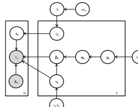
py,Z,v,nβ(k)o,τ,nα(k)o,nγ(k)o, λ|X =py|X,nβ(k)o,τp(Z|v)p(v|λ)p (λ|m0) ×pnβ(k)o|τ,nα(k)opnα(k)o|nγ(k)o ×p
n
γ(k)o|a0, b0
p (τ|c0, d0) . (10)
The graphical model that represents the dependence rela-tionships between all the parameters involved in this current mixture model is shown in Fig. 1. The shaded circles de-note observed variables; the unshaded circles dede-note unob-served variables. We have used a Gamma prior onλhaving a hyper-parameterm0. We have omitted the hyper-parameters a0,b0,c0,d0, andm0from the list of conditioning variables in the left side to avoid clutter. The individual distributions in
Figure 1. Graphical representation of the complete Bayesian
hier-archical model.
Eq. (10) are given below. y|X,nβ(k)o,τ∼
N
Y
n=1 K
Y
k=1
n
Nyn;x>nβ(k), τ
−1 k
oznk
(11a)
Z|v∼ N
Y
n=1 K
Y
k=1
(
vk k−1
Y
j=1
1−vj
)znk
(11b)
v|λ∼ K
Y
k=1
Beta(vk;1, λ) (11c)
λ∼Ga(λ;m0,1) (11d)
n
β(k)o|τk,
n
α(k)o∼ K
Y
k=1 D
Y
j=1 N
βj(k);0,τkαj(k)
−1
(11e)
τ∼ K
Y
k=1
Ga(τk;c0, d0) (11f)
n
α(k)o,
n
γ(k)o∼ K
Y
k=1 D
Y
j=1
InvGa α(k)j ;1, γj(k)
2
!
×Gaγj(k);a0, b0
(11g) 3.2 Accommodating “must link” constraints
Prior knowledge about must link constraints between pairs of data-points can be enforced via an MRF prior on the indica-tor variableszn, where each data-point is considered a node and each constraint between a pair of data-points is regarded as an edge between the respective nodes. We denote the col-lection of edges byCand the MRF prior is given by Eq. (4). We define the energy function as:
H zi,zj=
(
−1, z>i zj=1 and(i, j )is ML
Here ML means must link. This prior encourages similar val-ues of indicator variableszi andzj if they happen to share a “must link” edge. Since the MRF prior is assigned only on the indicator variables Z, it only alters Eq. (11b) and the new prior on Z is given by
Z|v∼ 1
Zexp
−
X
(i,j )∈C
H zi,zj
× N Y
n=1 K
Y
k=1
(
vk k−1
Y
j=1
1−vj
)znk
. (13)
3.3 Variational inference
Let us consider all the unknown parameters in our model as latent variables and denote all the latent variables by H= {Z,v, {β(k)}, τ,{α(k)}, {γ(k)}, λ}. Moreover, from now on, we will ignore feature variables X from the list of conditioning variables as they are observed. Using Jensen’s inequality, we can find a lower bound of the log-marginal lnp(y)which is given as
lnp(y) >
Z
q(H)ln
p(y,H)
q(H)
dH (14)
for any arbitrary distributionq(H). The variational inference is performed by restrictingq(H)within a parametric family so that the maximization of the lower bound given in Eq. (14) is tractable. We consider only thoseq(H)that factorize over some disjoint groups of the component random variables of H in the following way:
q(H)= L
Y
j=1
qj hj. (15)
We can now maximize the lower bound given in Eq. (14) with respect to each componentqj(hj)in Eq. (15) and obtain the parametric form ofqj(hj)given by
qj∗ hj=
exp Ei6=j
lnp (y,H)
R
exp Ei6=jlnp(y,H)dhj
, (16)
where the expectation is taken with respect to all the other factors{qi}fori6=j. It can be shown that theq(H)obtained this way is the closest approximation of the actual posterior
p(H|y)in terms of KL-divergence out of all possible alterna-tives of the form given by Eq. (15). Therefore this is a deter-ministic but approximate posterior inference method, unlike stochastic inference methods such as MCMC, which samples from the actual posterior. However, variational inference is much faster and approximates the true posterior reasonably well for practical purposes.
Once we apply Eq. (16) to the joint distribution described in Eqs. (10) and (11), we can get the update equations for the approximate posterior distributions for each of the latent variables involved.
1. Distribution ofz:
qZ(Z)=
Y
V∈V
1 ZV exp −X (i,j )∈C
i,j∈V
H zi,zj
Y
n∈V K
Y
k=1 ρnkznk
#
(17)
with
ρnk=
rnk
P
k
rnk
(18)
lnrnk= 1
2hlnτki − 1 2ln 2π−
hτki 2
yn2−2hβ(k)i>xnyn+x>nhβ(k)
β(k)
>
ixn
+ hlnvki + k−1
X
j=1
hln 1−vj
i. (19)
2. Distribution of{β(k)}:
qβ
n
β(k)o= K
Y
k=1
Nnβ(k)o;µk, 6(k) (20)
with
6(k)= hτki N
X
n=1
xnx>nE[Z]nk+ hτki
diaghα(k)i
−1
(21)
µk=6(k)
N
X
n=1
xnynE[Z]nk
!
hτki. (22)
Here diag(hα(k)i) corresponds to the LASSO (Tibshirani, 1994) shrinkage. The moments are given by1
hβ(k)i =µk;
βp(k)2
=6pp(k)+µ2kp
hβ(k)β(k)
>
i =6(k)+µkµ>k.
3. Distribution ofτ:
qτ(τ)= K
Y
k=1
Ga(τk;ck, dk) (23)
1hf (s)imeans expected value off (s)with respect to the
with
ck=c0+ 1 2
N
X
n=1
E[Z]nk+p
!
(24)
d=d0+ I 2+ J 2 (25) where I = N X
n=1
yn2E[Z]nk−2E[Z]nkx>nynhβ(k)i
+E[Z]nkx>nhβ(k)β(k)
> ixn J = D X
p=1
D
α(k)p E
βp(k)2
.
The relevant moments are
hτki =ck/dk andhlnτki =ψ (ck)−ln(dk) . 4. Distribution ofv
qv(v)= K
Y
k=1
Beta(vk;ξk, κk) (26)
with
ξk=1+ N
X
n=1
E[Z]nkandκk= hλi + K
X
j=k+1 N
X
n=1 E[Z]nj.
Relevant moments are given by hlnvki =ψ (ξk)−ψ
(ξk+κk)andhln(1−vk)i =ψ (κk)−ψ (ξk+κk). 5. Distri-bution of{α(k)}:
qα
n
α(k)o= K
Y
k=1 D
Y
p=1
InvGaussian
α(k)p ;gkp, hkp (27)
with
gjk=
v u u u u t D
γj(k)E
hτki
βj(k)
2
hkj=
D
γj(k)
E
where InvGaussian(α(k)j ; gkj, hkj)denotes inverse Gaussian distribution with meangkjand shape parameterhkjhaving the
following density function.
pIG
αj(k);gjk, hkj
= v u u u t
hkj
2πα(k)j 3
×exp
−
hkjα(k)j −gkj 2
2gjk2αj(k)
αj(k)>0
The relevant moments are given by
D
αj(k)
E
=gjkand
αj(k)
−1
=
gkj
−1
+
hkj
−1
.
6. Distribution of{γ(k)}:
qγ({γ(k)})= D
Y
p=1
Gaγj(k);ajk, bkj
(28)
with
ajk=a0+1 bkj=b0+
1 2
α(k)j −1
and the relevant moment ishγj(k)i =akj/bkj. 7. Distribution of
λ:
qλ(λ)=Ga(λ;u, w) (29)
where
u=m0+K; w= − K
X
k=1
hln(1−vk)i.
Relevant moment ishλi =u w.
The first part of the variational posterior of qZ(Z) in Eq. (17) arises from the MRF prior and contributes towards enforcing “must link” constraints. Note thatV in Eq. (17) is a set of sets andV is a component set of connected nodes within V. Basically, V denotes the set of connected com-ponents within the constraint graph described in Sect. 3.2. Therefore the partition function ZV needs to be computed only for the connected components, not for the entire graph. ComputingZV becomes tractable if the connected compo-nents are small (i.e., the constraint set is sparse).
component by computing the probabilities of each possi-ble state combination and summing the probability-weighted state matrices. The partition function is computed by sum-ming the exponentiated sum of energy function of each state matrix. Note that isolated nodes (not part of any connected components) will not need theirρnk updated.
The parameters of each of the distributions has depen-dency on moments of one or more of the other variables. We therefore find a locally optimum solution via an iterative pro-cess that starts with random initial values of the relevant mo-ments and stops when the indicator variables Z stop chang-ing. Note that once the approximate solution is reached, we can compute the marginal distributions over coefficientsβp(k) which is a Gaussian with mean µ(k)p and variance6pp(k) for eachk. We can thereby perform attest to determine whether the corresponding feature has a non-zero coefficient. 3.4 Computational considerations
One computational bottleneck of the proposed VB algorithm is the inversion of theD×Dmatrix in Eq. (21). IfD < N, then faster matrix inversion can be achieved by first apply-ing a Cholesky decomposition and then invertapply-ing the result-ing upper triangular matrix. However, ifD > N, we can first apply a fast (approximate) singular value decomposition on
6(k)−1and then use Woodbury matrix inversion identity so that we now have to invert aN×N matrix instead.
We have truncated the infinite DP at K=20 for most of our experiments. The speed of the algorithm can be further improved by parallelizing the updates for each ofK compo-nents, which is straightforward as they are updated indepen-dent of each other. Another major computational challenge was the MRF updates. Apart from controlling the maximum size of the connected components, we parallelized the MRF updates over each subgraph by making the state generation independent of the previous state.
4 Experiments
We have evaluated our method on both synthetic and climate data sets. Typical values used for the hyper-parameters were
a0=b0=c0=d0=0.01 and λ=1. Selecting these values within a reasonable range does not affect the results signifi-cantly. We made sure that the cardinality of the largest con-nected component in the constraints graph never exceeds 8. 4.1 Synthetic data set
We compared the performance of both constrained and un-constrained versions of our method with the non-parametric mixture of linear regression (NPMLR) model without any regularization. We set up three experiments: (1) to test whether or not our algorithm can learn the correct number of clusters; (2) to evaluate the effect of constraints; and (3) to check the sensitivity of our approach to noise.
For all our experiments involving synthetic data, we used
N=1000 data-points andD=30 features. In our first set of experiments we tested our method forK=2 . . . 5 actual clusters. Each column of theN×Dinput matrix X is gen-erated from a uniform distribution. For each value ofK, we partitioned the input matrix X inK equal parts X1. . . XK. Then for each partition Xk(k=1 . . . K), we generate sparse coefficientsβk by randomly selecting 10 out of 30 compo-nents to be non-zero. We assign a value of 5k(wherekis the index of the cluster,k=1, . . . ,K) to the non-zero compo-nents within thekth cluster so that two clusters are distinctly identifiable in case the indices of non-zero components of the clusters are the same. We then generate the outputyk for the
kth cluster using the linear regression model of Eq. (1). The fixed noise varianceτk−1for the first experiment was gener-ated by randomly choosing a number between 0 and 0.1 to introduce diversity. A final data set was obtained by merg-ing {Xk,yk} for all k=1 . . . K. The process is repeated 30 times and mean and variance of the evaluation metrics were reported in the form of error bars for each value ofK
in Fig. 2. For all these experiments, the total number of con-straints was kept at 20 per cluster while the size of the largest subgraph was kept below 7.
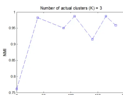
The second experiment was performed to evaluate the ef-fect of number of “must link” constraints on the performance of the constrained version of the algorithm. Here, the actual number of clusters was fixed atK=3 along with the base noise variance (0.1) and the number of constraints per clus-ter was varied from 0 to 30 incremented by 5, although the actual number of constraints may be less since we removed some constraints to achieve sparsity in the constraint graph. The result is reported in Fig. 3.
In our third experiment, we evaluated the effect of noise on the performance of our algorithm. Again, we kept the num-ber of clusters fixed atK=3 and the number of constraints fixed at 20 per cluster (for the constrained version). We varied the base noise level in each cluster from 0 to 0.5 and added a randomly generated value between 0 and 0.1 with the base noise level for each cluster to maintain diversity among the clusters. Average and variance of 30 repetitions are reported in Fig. 4.
4.1.1 Evaluation metrics
We measured two aspects of the performance of our algo-rithm. First,we measured whether it can cluster the data-points correctly. We put a data-point into one of the pos-sible 20 components (since we truncated the infinite DP at
Figure 2. Left panel: ability of nonparametric unregularized and sparse regressions (unconstrained and constrained) to correctly identify
clusters in presence of increased number of actual components in the data. Right panel: ability of nonparametric unregularized and sparse regressions (unconstrained and constrained) to correctly retrieve the sparse structure within each cluster.
Figure 3. Performance of the constrained version of the algorithm
(in terms of NMI (more the better)) with number of “must link” constraints.
ones. Note that the estimated cluster indices (a value be-tween 1 and 20) may not correspond directly to the actual cluster indices (a value between 1 to actual value ofK) since the variational inference algorithm is not aware of the actual order of the cluster indices (e.g., actual cluster index 1 may correspond to estimated cluster index 9). So we use a met-ric called normalized mutual information (NMI) that evalu-ates the match between estimated cluster membershipscˆand actual ones c without needing direct correspondence. NMI is given by NMI(c, cˆ)=H (√c)−H (c|ˆc)
H (c)H (cˆ) , whereH (
·)is the en-tropy. Higher NMI values mean that the clustering results are more similar to ground-truth. The metric reaches its maxi-mum value of one when there is perfect agreement.
A second metric is used to evaluate the quality of the sparse regression model estimated within each discovered cluster. Here we are only interested in finding whether our
algorithm picks the non-zero coefficients correctly. We use
F score to measure the match between actual and estimated non-zero coefficients within each cluster.F score for thekth component is given byFk=Pk2Pk+RkRk, wherePk is the preci-sion andRkis the recall of the estimated coefficients for the
kth component. We reported the average ofFkvalues over all components discovered by our algorithm. Unlike the previ-ous metric, here we need to know the direct correspondence between the cluster indices so that we can match the actual and estimated coefficient vectors. We developed an algorithm to find such a correspondence based on bipartite matching. 4.1.2 Discussion of results
We can see the performance of all three algorithms are com-parable in terms of identifying the clusters correctly, al-though the NMI value of NPMLR degrades significantly for K=5. However, as desired, our method outperforms NPMLR in terms of correctly retrieving the sparse structure of regression coefficients within each cluster. There is a gen-eral downward trend of performance for all algorithms with increasing number of actual components in the data. This is an inherent problem with the DPM models as it tends to at-tach each new data-point to the largest current component, thereby favoring models with fewer components. Also, as the number of actual components grows, the probability of two components being similar increases.
Figure 4. Left panel: ability of nonparametric unregularized and sparse regressions (unconstrained and constrained) to correctly identify
clusters (indicated by NMI) with increasing noise. Right panel: ability of nonparametric unregularized and sparse regressions (unconstrained and constrained) to correctly retrieve the sparse structure within each cluster (indicated by averageFscore).
our method is relatively robust to added noise, a major chal-lenge with the real data sets, especially in terms of correctly identifying the sparse structure.
4.2 Feature selection for downscaling rainfall
A grand challenge in climate science relevant for adapta-tion and policy remains our inability to provide credible stakeholder-relevant “statistical downscaling”, or to develop statistical techniques for more accurate, precise and inter-pretable high-resolution projections with lower-resolution climate model data (Benestad et al., 2008). Regression mod-els of statistical downscaling (Benestad et al., 2008; Ghosh, 2010) work by first selecting a set of climate variables that have information about the target variable, and then fitting a regression model to predict the target variable at higher res-olution. In this application, selecting the right set of predic-tors is as important as building a prediction model since even a good prediction with a model that is physically not inter-pretable is less desirable as it may not generalize well. We focus on the feature selection problem for statistical down-scaling of annual average rainfall. The use of annual averages reduces the amount of noise in the observed rainfall data, which enables us to examine the robustness of our methods with less ambiguity.
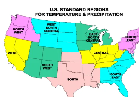
Existence of multiple states or patterns is acknowledged in regression-based statistical downscaling literature for rain-fall (e.g., Kannan and Ghosh, 2010) where parametric meth-ods such ask-means were used to find distinct clusters. Here we used our model to simultaneously find clusters, if any, and select features for the purpose of statistical downscaling of station-observed annual average rainfall over two climato-logically homogeneous regions over the continental US. Fig-ure 5 shows the climatologically homogeneous regions over the US.
Figure 5. Map showing climatologically homogeneous regions over
continental US.
Since rainfall follows a log-normal distribution (Kedem and Chiu, 1987), the target variable we used is logarithm of annual average rainfall. In Fig. 6, we show the distribution of average rainfall over all sites in western US before and after taking the logarithm.
Figure 6. Left panel: distribution of average rainfall over all sites in the western US. Right panel: distribution of average rainfall after
transformation.
Table 1. Potential features used for statistical downscaling of rainfall.
Atmospheric (Easterling et al., 1996; Mesinger et al., 2006)
MATmax Mean Annual Maximum Temperature
DJFTmax Mean Winter Maximum Temperature
MAMTmax Mean Spring Maximum Temperature
JJATmax Mean Summer Maximum Temperature
SONTmax Mean Autumn Maximum Temperature (Easterling et al., 1996)
SLP Sea Level Pressure
CAPE Convective Available Potential Energy (Mesinger et al., 2006)
Climate indices (NOAA, 2014)
NAO North Atlantic Oscillation
EA East Atlantic Pattern
WP West Pacific Pattern
EPNP East Pacific/North Pacific Pattern
PNA Pacific/North American Pattern
EAWR East Atlantic/West Russia Pattern
SCA Scandinavia Pattern
TNH Tropical/Northern Hemisphere Pattern
POL Polar/Eurasia Pattern
PT Pacific Transition Pattern
PDO Nino 1+2, Nino 3, Nino 3.4, Nino 4
SOI Southern Oscillation Index
PDO Pacific Decadal Oscillation
NP Northern Pacific Oscillation
TNA Tropical/Northern Atlantic Index
TSA Tropical/Southern Atlantic Index
WHWP Western Hemisphere Warm Pool
GlobalMeanTemp Global Mean Temperature Anomaly (NOAA, 2014)
Climate indices are global variables that represent large-scale signals in climate variables. A list of covariates used for each category is given in Table 1. A dependence on any of these variables roughly indicates rainfall due to large-scale circulation. In addition to these covariates, we have used el-evation as a potential feature which falls under none of the above categories. This is the only feature that represents the geography of the region.
Figure 7. Left panel: location of stations and their cluster membership in the western region. Right panel: location of stations and their cluster
membership in the northwestern region.
NV) and northwest (WA, OR, ID) regions are shown by gray shaded areas over the US map in Fig. 7 (left and right panels, respectively).
Results and discussion
We applied spatial “must-link” constraints among pairs of data-points from the same location. Ideally, if there are
n points in a cluster, we will be required to put n2 con-straints to cover all pairs of data-points. To reduce complex-ity, initially we kept only those constraints that connect data-points from consecutive years. However, this reduced set of constraints proved to be too restrictive and all data-points tended to merge into a single cluster. So, we kept remov-ing the constraints in an intuitive manner until more than one cluster emerged for a region. We found more than one clus-ter for all regions except the southern region. We stopped removing constraints until new clusters stopped emerging for a region. Here we show only the clusters in the western and northwestern regions, since the majority of stations were mostly split into obtained clusters in these regions. In other regions, almost all stations had mixed membership. We as-sign a station to a cluster if more than 80 % of its data-points belong to that cluster.
A quick look at the histogram of target variable (right panel in Fig. 6) also supports the possibility of two distinct rainfall modes in the region. As mentioned earlier, we ob-tained one sparse linear model for each of the discovered components within a region. Since a non-zero coefficient in the sparse model implies dependence on the corresponding covariate, we can obtain interesting insights about the depen-dence of average rainfall on various atmospheric and climate indices from the coefficients of the individual sparse mod-els within each cluster. Interestingly, in the northwest region there is only a single member station in the first component that exhibits dependence on the local temperature variables and SLP, whereas the larger cluster shows dependence on a larger number of climate indices. In the western region, the
first cluster shows dependence on local temperature variables and the second cluster shows more dependence on large-scale variables. Both clusters show dependence on elevation. While dependence on large-scale indices is not surprising for both these coastal regions due to the known effect of westerlies, dependence of smaller clusters (especially in the northwest) on local variables may hint at the existence of some regional small-scale atmospheric mechanisms. While spatially coherent clusters are more likely to occur in na-ture, geographical features such as mountains and lakes and even man-made structures such as large dams and reservoirs may abruptly disturb the spatial smoothness of clusters, since their presence may alter the climate pattern of the nearby ar-eas with respect to the surrounding regions. However, before we can build statistical downscaling models, more rigorous statistical and physical analysis is required based on these preliminary insights obtained using our method. The clusters discovered here, and the corresponding covariates, can be uti-lized to develop individual non-linear prediction models per cluster.
to distinguish among major categories of relationships even though some of them may be lumped together.
5 Conclusions
In this paper, we propose a nonparametric Bayesian mix-ture of sparse regression models for simultaneous cluster-ing and discovery of covariates within each cluster uscluster-ing a DP mixture model. Moreover, our model can accommodate prior knowledge about “must link” constraints between the pair of data-points using a Markov Random Field prior on the cluster membership variables. Our major contribution is to develop an efficient and scalable variational inference al-gorithm for inference on the fully Bayesian model. We ap-plied our method to both synthetic and real climate data and successfully discovered multiple underlying behaviors in the data. Preliminary results of applying our method to feature selection for statistical downscaling of rainfall show promise towards finding new climate insights with approate caveats. Going forward, we would like to incorporapproate pri-ors for diversity among the clusters in order to discourage merging of close but dissimilar clusters. We intend to extend our model for predictive analysis and build a full-scale statis-tical downscaling method using the features selected by the current model.
Acknowledgements. This work was funded by the NSF Expe-ditions in Computing grant “Understanding Climate Change: A Data Driven Approach”, award number 1029166. We thank the anonymous referees for their valuable suggestions and comments.
Edited by: V. Kumar
Reviewed by: three anonymous referees
References
Antoniak, C.: Mixtures of Dirichlet processes with applications to Bayesian nonparametric problems, Ann. Stat., 2, 1152–1174, 1974.
Bader, D. C., Covey, C., Gutkowski Jr., W. J., Held, I. M., Kunkel, K. E., Miller, R. L., Tokmakian, R. T., and Zhang, M. H.: Climate Models: An Assessment of Strengths and Limitations, US Cli-mate Change Science Program Synthesis and Assessment Prod-uct 3.1, Department of Energy, Office of Biological and Environ-mental Research, 124 pp., available at: http://pubs.giss.nasa.gov/ docs/2008/2008_Bader_etal_1.pdf (last access: 20 July 2014), 2008.
Basu, S., Bilenko, M., Banerjee, A., and Mooney, R.: Probabilis-tic semi-supervised clustering with constraints, J. Mach. Learn. Res., 71–98, 2006.
Benestad, R., Hanssen-Bauer, I., and Chen, D.: Empirical-Statistical Downscaling, World Scientific Publishing Company, New Jer-sey, London, 2008.
Bishop, C. and Svenskn, M.: Bayesian hierarchical mixtures of ex-perts, in: Uncertainty in Artificial Intelligence, Morgan Kauf-man, San Francisco, CA, 57–64, 2002.
Blei, D. M. and Jordan, M. I.: Variational inference for Dirichlet process mixtures, Bayesian Anal., 1, 121–143, 2006.
Easterling, D. R., Karl, T. R., Mason, E. H., Hughes, P. Y., and Bowman, D. P.: United States Historical Climatology Net-work (USHCN) Monthly Temperature and Precipitation Data, Tech. rep., Oak Ridge National Laboratory, US Department of Energy, Oak Ridge, Tennessee, available at: http://cdiac.ornl. gov/epubs/ndp/ushcn/ushcn.html (last access: 2 April 2014), 1996.
Ebtehaj, A. M., Foufoula-Georgiou, E., and Lerman, G.: Sparse reg-ularization for precipitation downscaling, J. Geophys. Res., 117, 1–12, doi:10.1029/2011JD017057, 2012.
Ferguson, T.: A Bayesian analysis of some nonparametric problems, Ann. Stat., 1, 209–230, 1973.
Geman, S. and Geman, D.: Stochastic relaxation, Gibbs distribu-tions, and the Bayesian restoration of images, IEEE T. Pattern Anal., PAMI-6, 721–741, 1984.
Ghosh, S.: SVM-PGSL coupled approach for statistical downscal-ing to predict rainfall from GCM output, J. Geophys. Res., 115, D22102, doi:10.1029/2009JD013548, 2010.
Greene, A. M., Robertson, A. W., Smyth, P., and Triglia, S.: Down-scaling projections of Indian monsoon rainfall using a nonhomo-geneous hidden Markov model, Q. J. Roy. Meteorol. Soc., 137, 347–359, 2011.
Hespanha, J. P.: An efficient MATLAB Algorithm for Graph Parti-tioning, Tech. rep., University of California, Santa Barbara, avail-able at: http://www.ece.ucsb.edu/~hespanha/techrep.html (last access: 2 April 2014), 2004.
Ishwaran, H. and James, L. F.: Gibbs sampling methods for stick-breaking priors, J. Am. Stat. Assoc., 96, 161–173, 2001. Kannan, S. and Ghosh, S.: Prediction of daily rainfall state in a river
basin using statistical downscaling from GCM output, Stoch. Env. Res. Risk. A., 25, 457–474, doi:10.1007/s00477-010-0415-y, 2010.
Kedem, B. and Chiu, L. S.: On the lognormality of rain rate, P. Natl. Acad. Sci. USA, 84, 901–905, 1987.
Knutti, R. and Sedláˇcek, J.: Robustness and uncertainties in the new CMIP5 climate model projections, Nat. Clim. Change, 3, 369–373, doi:10.1038/nclimate1716, 2013.
Kumar, D., Kodra, E., and Ganguly, A. R.: Regional and seasonal intercomparison of CMIP3 and CMIP5 climate model ensembles for temperature and precipitation, Clim. Dynam., 43, 2491–2518, doi:10.1007/s00382-014-2070-3, 2014.
Mesinger, F., DiMego, G., Kalnay, E., Mitchell, K., Shafran, P. C., Ebisuzaki, W., Jovi´c, D., Woollen, J., Rogers, E., Berbery, E. H., Ek, M. B., Fan, Y., Grumbine, R., Higgins, W., Li, H., Lin, Y., Manikin, G., Parrish, D., and Shi, W.: North Ameri-can regional reanalysis, B. Am. Meteorol. Soc., 87, 343–360, doi:10.1175/BAMS-87-3-343, 2006.
NOAA: Climate Indices: Monthly Atmospheric and Ocean Time Series, available at: http://www.esrl.noaa.gov/psd/data/ climateindices/list/, last access: 2 April 2014.
Phatak, A., Bates, B., and Charles, S.: Statistical
down-scaling of rainfall data using sparse variable
selec-tion methods, Environ. Modell. Softw., 26, 1363–1371, doi:10.1016/j.envsoft.2011.05.007, 2011.
Ross, J. and Dy, J.: Nonparametric Mixture of Gaussian Processes with Constraints, The 30th International Conference of Machine Learning, Atlanta, GA, 2013.
Sethuraman, J.: A constructive definition of Dirichlet priors, Stat. Sinica, 4, 639–650, 1994.
Tarjan, R.: Depth-first search and linear graph algorithms, SIAM J. Comput., 1, 146–160, 1972.
Tibshirani, R.: Regression shrinkage and selection via the LASSO, J. Roy. Stat. Soc. B, 58, 267–288, 1994.