www.clim-past.net/9/2365/2013/ doi:10.5194/cp-9-2365-2013
© Author(s) 2013. CC Attribution 3.0 License.
Climate
of the Past
Pre-LGM Northern Hemisphere ice sheet topography
J. Kleman1, J. Fastook2, K. Ebert1, J. Nilsson3, and R. Caballero3
1Department of Physical Geography and Quaternary Geology, Stockholm University, Bolin Centre for Climate Research,
10691, Stockholm, Sweden
2Department of Computer Science, University of Maine, Orono, ME 04469-5790, USA
3Department of Meteorology, Stockholm University, Bolin Centre for Climate Research, 10691, Stockholm, Sweden
Correspondence to: J. Kleman (kleman@natgeo.su.se)
Received: 15 April 2013 – Published in Clim. Past Discuss.: 17 May 2013
Revised: 13 August 2013 – Accepted: 10 September 2013 – Published: 22 October 2013
Abstract. We here reconstruct the paleotopography of Northern Hemisphere ice sheets during the glacial maxima of marine isotope stages (MIS) 5b and 4.We employ a com-bined approach, blending geologically based reconstruction and numerical modeling, to arrive at probable ice sheet ex-tents and topographies for each of these two time slices. For a physically based 3-D calculation based on geologically de-rived 2-D constraints, we use the University of Maine Ice Sheet Model (UMISM) to calculate ice sheet thickness and topography. The approach and ice sheet modeling strategy is designed to provide robust data sets of sufficient resolu-tion for atmospheric circularesolu-tion experiments for these previ-ously elusive time periods. Two tunable parameters, a tem-perature scaling function applied to a spliced Vostok–GRIP record, and spatial adjustment of the climatic pole position, were employed iteratively to achieve a good fit to geological constraints where such were available. The model credibly reproduces the first-order pattern of size and location of geo-logically indicated ice sheets during marine isotope stages (MIS) 5b (86.2 kyr model age) and 4 (64 kyr model age). From the interglacial state of two north–south obstacles to atmospheric circulation (Rocky Mountains and Greenland), by MIS 5b the emergence of combined Quebec–central Arc-tic and Scandinavian–Barents-Kara ice sheets had increased the number of such highland obstacles to four. The number of major ice sheets remained constant through MIS 4, but the merging of the Cordilleran and the proto-Laurentide Ice Sheet produced a single continent-wide North American ice sheet at the LGM.
1 Introduction
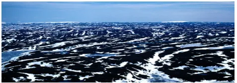
Fig. 1. The Terra Nivea and Grinnell ice caps (on the skyline) rise
only about 200 m above the level 600 m-elevation plateau of Meta Incognita Peninsula, Baffin Island. The setting is typical of the in-ception and build-up areas of North American ice sheets in the mainly lowland Laurentide area during the early part of the last glacial cycle.
circulation changes have caused mass balance patterns that left Alaska largely ice-free throughout the last glacial cy-cle, the high-elevation Cordilleran region only ephemerally glaciated (Clague, 1989), but the almost entirely lowland Laurentide area (Fig. 1) persistently glaciated? Did down-stream influence of the North American ice sheet topogra-phy on the atmospheric circulation contribute to southwest-ward migration of the mass center of the Eurasian Ice Sheet? Amplification of the effects of modest insolation changes appears necessary to explain ice sheet build-up in the Lau-rentide area (Otieno and Bromwich, 2009). In addition, the topographical and albedo changes caused by ice sheets are likely part of the non-linear response of the climate system to the insolation changes that pace glacial cycles. Considerable progress is being made in establishing the general response characteristics of the climate system by statistical analysis of the global ice volume response to insolation forcing (Lourens et al., 2010; Imbrie et al., 2011). However, to understand the impact of changing topography on atmospheric circulation and the growth of ice sheets, also the location, extent and height of individual ice sheets must be known.
Improved understanding of Northern Hemisphere paleoto-pography of intermediate-sized ice sheets can, if combined with the relevant array of paleoclimatic proxy data, yield a valuable calibration data set for tuning and comparison of climate models at global ice volumes smaller than the LGM case normally used (Kageyama et al., 1999; Otto-Bliesner et al., 2006). The present situation, in which research focus has been on two climatic end members, largely precludes re-search on non-linear responses to ice sheet build-up. Over the last decades evidence has accumulated that ice sheet extent and volume varied more drastically over shorter time scales than previously thought, and a new paradigm of highly dy-namic ice sheets has emerged (Boulton and Clark, 1990). Of particular importance is the evidence for ice-free core ar-eas in Fennoscandia (Wohlfarth, 2010; Helmens and Engels, 2010), the consequence of which is that the Fennoscandian Ice Sheet had to be fully rebuilt from zero ice volume dur-ing each of the cold phases (MIS 5d, 4 and 2). From this
new paradigm, time and precipitation emerge as important limiting factors for the glacial development, and there is a need to explore the atmospheric circulation and conditions that allowed ice sheets to be fully rebuilt during the rela-tively short intervals of declining Northern Hemisphere high-latitude summer insolation.
Previous work
Reconstructions of the LIS at the LGM based on numerical ice sheet modeling have ranged from a thick monodome ice sheet (Denton and Hughes, 1981) to a relatively thin multi-domed ice sheet (Clark et al., 1996). More recent ice sheet models (Marshall et al., 2000; Tarasov and Peltier, 2004; Álvarez-Solas et al., 2011; Gregoire et al., 2012) agree that the LIS at the LGM exhibited a multi-domed shape with a complex configuration of ice streams and inter-stream ridges in peripheral areas. Likewise there is a convergence on the existence of frozen-bed core areas under the main domes, in line with was inferred from geomorphological evidence by Kleman and Hättestrand (1999). Few numerical model-ing exercises focus on, or include, the growth phase of the ice sheet (Huybrechts and T’siobbel, 1995; Charbit et al., 2007; Bintanja et al., 2002; Bonelli et al., 2009). Many of those that do so conflict with the geological evidence for ice sheet extent at the LGM, which is currently the prime avail-able “target” period for assessing the validity and credibility of the climates used in these numerical models. Common is too much ice cover in Alaska and the Mackenzie mountains (NW sector), areas that were largely ice-free at the LGM, and also continuous and massive glaciation of British Columbia instead of the geologically indicated ephemeral ice cover (Clague, 1989). These common problems are discussed at length in Bonelli et al. (2009). Most models are also unable to generate a southward extent of the Quebec Dome during ice sheet build-up that is sufficiently large to match the ge-ological evidence (Stea, 2004; Kleman et al., 2010). The re-cent ensemble-based reconstruction by Stokes et al. (2012) is focused on the build-up phase and represents a major step forward in understanding the dynamics of proto-Laurentide ice sheets. It was tuned on the basis of data for the post-LGM period, and the output for the pre-post-LGM stages are thor-oughly discussed in relation to geological data. One of the currently leading ice sheet models (ICE-5G, Peltier, 2004) is based on isostatic recovery rather than mass-balance-driven ice physics, and is unable to reconstruct pre-LGM conditions because of the time constants involved in isostatic recov-ery. An early attempt at a geologically and geomorpholog-ically constrained pre-LGM LIS model was presented by us some years ago (Kleman et al., 2002), and we here build on experience gained during that work.
of stratigraphic control for this time interval is much smaller than for the deglaciation period 21–8 kyr. The time interval is much longer, and can rarely be addressed with radiocarbon dates. In addition, almost all landforms and deposits created in this time interval have been subjected to overriding ice during the LGM and later stages, which in most cases has led to erosion or burial and therefore full or partial destruc-tion and reshaping, and to severe spatial fragmentadestruc-tion of the record compared to the records from the LGM and deglacial periods (Kleman et al., 2010). These difficulties add up to a major methodological challenge, and require a focus on only the first-order patterns in the evolution of ice sheets in this time interval. For the pre-LGM period it is not possible to achieve the spatial and temporal precision of post-LGM re-constructions (Dyke et al., 2002; Ehlers and Gibbard, 2003). We here present first-order paleotopographical data sets for the ice volume maxima of marine isotope stages 5b and 4, the two youngest build-up phases preceding the LGM. These reconstructions are meant to be relevant as topographic input for atmospheric circulation experiments; the data can and are intended to be used in modeling studies of the impact of these early ice sheet configurations on the large-scale atmospheric circulation. There is a considerable amount of literature con-cerning such studies for the LGM (e.g., Manabe and Broc-coli, 1985; Cook and Held, 1988), but much less attention has been devoted to understanding the pre-LGM atmospheric response. In particular, the atmospheric stationary waves, which are topographically forced and have wavelengths of a few 1000 km (Held et al., 2002), are of key importance in this context. The bed conditions, frozen or thawed, ex-ert some control on ice sheet thickness, but the finer-scale details of the ice sheet topography, although of importance for local climatic conditions, have a relatively weaker impact on the hemispheric-scale stationary waves. Accordingly, we have not tried to capture the details of ice sheet outline or in-ternal ice sheet dynamics, since the large-scale atmospheric flow is not critically dependent on such information. We have used the best available geological constraints on ice sheet ex-tent and, through numerical modeling, strived for first-order reconstructions that represent our current best understanding of location, extent and thickness in this time interval.
Our approach is not puristic. We do not regard geological data as an indisputable “truth” against which model output is evaluated. Instead, in line with Kleman et al. (2010), we ar-gue that discrepancies between “control” data and numerical modeling results can point to flaws in interpretation of data as well as deficiencies in the numerical modeling. We em-ploy both approaches here – geologically based reconstruc-tion and numerical modeling – to arrive at the most probable ice sheet extent and topography for each time slice.
2 Methods
Our strategy is governed by the intended end use of paleo-atmospheric circulation modeling. For that purpose a high-precision ice sheet outline is not crucial, but the existence or non-existence of an ice sheet in a certain location is impor-tant. It can be expected that small and thin ice sheets will not significantly affect the large-scale atmospheric circula-tion. Hence we are primarily concerned with capturing the main ice sheet features and ice sheets with a length of at least 1000 km.
The situation regarding data that spatially constrain pre-LGM ice sheets is very uneven for the respective glacia-tion centers, with a relatively good understanding in west-ern Eurasia; some effective constraints, albeit with poor dat-ing control, for the Laurentide Ice Sheet; and very little solid knowledge for the Cordilleran and Inuitian ice sheets in these time intervals.
We have here chosen to base our synthesis primarily on previous spatial reconstructions (Dredge and Thorleif-son, 1987; Clague, 1989; Clark et al., 1993; Kleman et al., 1997, 2010; Lundqvist, 2004; Svendsen et al., 2004; Mangerud, 2004; Winsborrow et al., 2004; Lambeck et al., 2006) that cover this time interval. A full consideration of primary morphological and stratigraphic data is offered in several of the key source publications. In compiling the set of 2-D modeling targets (Fig. 2), each corresponding to a certain time interval, we have used the following ap-proach: (i) where approximate consensus on ice sheet out-line exists, we have drawn an averaging and somewhat sim-plified outline; (ii) where clearly dissenting views exist, we have weighed the quality and amount of geological evidence and decided on what we consider the most likely alternative; and (iii) for an outline that is considered spatially reliable, but for which alternative age assignments exist, we have weighed the age options and chosen that which we consider to be the most probable one.
The generally poor understanding of pre-LGM extent of particularly the Cordilleran and Inuitian ice sheets constitutes a “missing ice sheet” problem. There is not sufficient, nor reliable enough, data to allow us to show ice sheets’ outlines in these areas on any of the panels in Fig. 2, yet embryonic or smaller ice sheets are very likely to have existed in these areas during the time intervals in question. To use the outlines shown in Fig. 2 as “hard” modeling targets (in which ice in areas marked as ice-free in Fig. 2 is regarded as indicating a poor model fit) would clearly be erroneous, and would have caused us to use inappropriate forcing of the model to keep ice out of these areas.
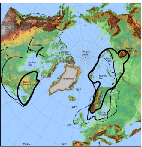
Fig. 2. The geological and geomorphological constraints (ice
mar-gin outlines) that were used in modeling paleotopography for glacial maxima during MIS 5b (heavy solid line) and 4 (thin solid line). LGM ice extent is indicated with stippled line. For source data and construction of outlines, see text.
to the two other major cold stages, MIS 4 and MIS 2 (the LGM). Given the similarity in global ice volume (Lisiecki and Raymo, 2005) and available sea level data (Lambeck et al., 2002) between the two stages, we consider it reasonable to regard this pattern as archetypical also for stage 5d.
3 Spatial extent of ice sheets based on geological evidence
3.1 North America
For the extent of North American ice sheets before the LGM, we have based our 2-D outlines primarily on the recent re-view by Kleman et al. (2010) and references therein, particu-larly Dredge and Thorleifson (1987), Clague (1989), Boulton and Clark (1990), Clark et al. (1993), and Stea et al. (2004). For the Keewatin sector of the Laurentide Ice Sheet there is good evidence for one or two, probably closely related, stages of a pre-LGM ice sheet with a dome center in the northern Keewatin or south-central Arctic region (Kleman et al., 2002, 2010; McMartin and Henderson, 2004). However, the east–west extents, maximum southerly extents, and ages are poorly constrained. Inferences about their pre-LGM age can be made on the basis of flow pattern and relation to other flow systems, but we know of no firm dating constraints. The flow patterns do indicate that both were dynamically inde-pendent of the Quebec Dome. The lineation evidence for this
ancestral northern Keewatin dome highlights the missing ice sheet problem. The lineation evidence for flow out of an an-cestral northern Keewatin/central Arctic dome is solid but covers only a restricted sector or corridor which lacks any to-pographic funneling. Glaciological considerations therefore require this lineation system to be only a fragment of a much wider flow pattern emanating from northern Keewatin or the south-central Arctic islands. Despite its limited area it thus indicates the existence of a full ice sheet, about whose east– west extent unfortunately not enough is known to warrant its full inclusion in Fig. 2. However, its minimum southward extent into the area of preserved traces is a viable modeling target.
In the Quebec sector, Kleman et al. (2002) assigned the “Atlantic” flow system, which indicates an ice divide closer to the Atlantic coast than any subsequent stage, to stage 5b or 5d. We consider it likely that this pattern characterized both stages and have therefore included it as a constraint for stage 5b. Regarding the Cordilleran Ice Sheet, Kleman et al. (2010) concluded that there was flow-trace evidence for “old” con-figurations with more easterly dispersal centers (Stumpf et al., 2000) than the ones that prevailed in near-LGM time, but constraints on age and outline are lacking. Hence, the Cordilleran Ice Sheet is one element of the missing ice sheet problem, and it appears very likely that this region was at least partly glaciated during MIS 5d, 5b, and 4, but there is simply not enough geological and geomorphological data to suggest an outline. Similarly, it appears likely that a proto-Inuitian ice sheet existed on the Queen Elizabeth Islands dur-ing these stages, but again there is not enough data to warrant the suggestion of a specific outline.
3.2 Eurasia
mainland Europe. The eastern margin of the Scandinavian Ice Sheet at this stage was approximately halfway between its stage 5b and LGM positions. The British Isles were glaciated during the LGM, but we acknowledge great uncertainty re-garding the ice extent and possible confluence with Scandi-navian ice during stage 4. Although volumetrically small, the southwestward lengthening of the Eurasian Ice Sheet that a British Ice Sheet may have provided was potentially impor-tant for atmospheric circulation changes.
4 Model and modeling strategy
4.1 Model
We employ the University of Maine Ice Sheet Model (UMISM), which consists of a time-dependent finite-element solution of the coupled mass, momentum, and energy con-servation equations (Fastook and Chapman, 1989; Fastook, 1993) with a broad range of applications (Holmlund and Fas-took, 1995; Johnson and FasFas-took, 2002; Kleman et al., 2002). The primary input to the model is present bedrock topog-raphy, the surface mean annual temperature, the geothermal heat flux, and the net mass balance, all defined as functions of position. The solution consists of ice thicknesses, surface elevations, column-integrated ice velocities, the temperature field within the ice sheet, the amount and distribution of wa-ter at the bed resulting from basal melting, and the amount of bed depression resulting from the ice load.
The primary solution is of the mass conservation equation. The required column-integrated ice velocities at each point in the map plane are obtained by numerically integrating the momentum equation through the depth of the ice. Stress is a function of depth and related to strain rates through the flow law of ice. The temperature, on which the flow law ice hard-ness depends, is obtained from a 1-D finite-element solution of the energy conservation equation, which includes internal heat generation produced by shear with depth and sliding at the bed.
Ice hardness is calculated from these modeled internal temperatures and is based on ice hardness parameterizations from Paterson (1994), modified by an appropriate flow en-hancement factor designed to accommodate fabric and debris content known to differ between hemispheres (Huybrechts, 1990; Ma et al., 2010). Sliding at the bed follows Weert-man (1964, 1969) and WeertWeert-man and Birchfield (1982). The amount of water at the bed is a function of the internal tem-perature calculation. In addition, a 2-D solution for conser-vation of water at the bed allows for movement of the basal water down the hydrostatic pressure gradient (Johnson and Fastook, 2002).
While this is a shallow-ice approximation model where only the basal shear stress is considered, we do include a longitudinal thinning strain rate at the grounding line that models ice drawn into a buttressing ice shelf that itself is not
explicitly modeled. This thinning rate is added to the mass balance source term of the mass conservation equation only in elements that contain a grounding line, and it is propor-tional to grounding line thickness raised to the fourth power (Weertman, 1957). We modify this rate by a parameter we call the “Weertman” that ranges from 0 (full buttressing, no thinning into the ice shelf) to 1 (no buttressing, thinning at a rate commensurate with an unconfined floating ice slab). While not used in this exercise, and assumed to be nominally zero everywhere inside the continental shelf break, this pa-rameter can be used to control the advance and retreat of a marine margin.
4.2 Model setup
With surface temperature and mass balance obtained from measured data, from GCM results, or from a climate param-eterization, the model can be run with no more input than the specified bedrock topography, in what can be called a “free-running mode”. However, it can also be tightly con-strained by geological and glaciological data when such data are available. Ice margin positions can be specified and ar-eas of basal sliding can be derived from the distribution of basal temperatures, or they can be specified by the presence of erosional features on exposed landscapes. In this exercise all of Eurasia and most of North America are free running. The exception is that in North America glaciation of the to-pographically high Rocky Mountains is suppressed.
We used a relatively coarse grid spacing of 95 km, suit-able for the broad picture we are attempting to produce for use in atmospheric circulation modeling. A regular rectangu-lar grid with 10 000 (100×100) nodal points spanning the Northern Hemisphere was used. We divided this into a West-ern Hemisphere grid and an EastWest-ern Hemisphere grid so that climatic adjustment could be applied separately to the two hemispheres to obtain the best fit. The time step required at this resolution was 10 yr.
998
Figure 3
999 1000 1001
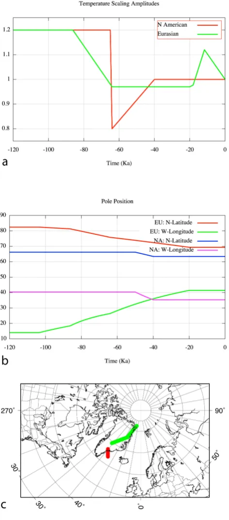
Fig. 3. (a) The temperature forcing, spliced Vostok and GRIP
records, used for the modeling. (b) A time-dependent scaling was used to fit ice sheet size to geological constraints. See text and Fig. 4 for full explanation. (c) Modeled ice volumes for the North Ameri-can and Eurasian domains of the model, respectively.
one can see by comparing the SPECMAP-stacked oxygen-isotope record (Imbrie et al., 1984), itself thought to rep-resent global sea level and the basis for the definitions of the stages we are investigating, that there is better agree-ment with the Vostok record than with the GRIP core. This
appears to also be true with regards to a terrestrial oxygen-isotope record from North America, DH-11 (Landswehr et al., 1997), which may better correlate with Vostok than with GRIP. However, the Vostok core does not strongly record the Allerøod warming nor the Younger Dryas cold reversal whose impact is well documented in Northern Hemisphere ice sheet retreat records. While behavior of the retreating ice sheets is not part of this study, we did observe marginal posi-tions at the Younger Dryas as one of our targets for goodness of fit. We therefore employed a spliced Vostok–GRIP record, Vostok prior to 20 KBP during which our target time slices occur, and GRIP during the deglaciation for comparison with Younger Dryas marginal positions.
The use of a global temperature such as our spliced GRIP-Vostok record is common in reconstruction of ice sheet glaciation cycles, and indeed provides an important timing and amplitude to whatever climate parameterization is used. Since we are fitting our modeled ice sheets to geologically constrained areal footprints, we regard it as justified to adjust this global temperature proxy with a temporally variable and regional scaling factor, shown in Fig. 4a, in order to recre-ate ice sheet sizes compatible with the constraints. This was done by systematically adjusting the scaling factor to yield a still stand, or maximum in the areal extent, that matched the margin positions outlined in Fig. 2 within a time range appropriate for the particular stage (we also had targets at MIS 5d and at the Younger Dryas, as well as the 5b, 4, and 2 (LGM) stages reported here). Once a target configuration has been met, the prior temporal variation is frozen, and sys-tematic adjustment from that still stand forward proceeds to the next target configuration.
Deviations from the core proxy do not exceed 1◦C for Eurasia and 1.5◦C for North America. For both North Amer-ica and Eurasia it was necessary to increase amplitudes by a factor of 1.2 (a decrease in temperature by approximately 1◦C) in the early part of the glacial cycle in order to match the target ice sheet areal footprints. The scaling amplitudes were reduced for both ice sheets during and after stage 4, in order not to overshoot documented stage 2 ice mar-gins (1.4◦C warmer briefly for North America and 0.25◦C warmer for Eurasia almost to the LGM).
Fig. 4. Primary tuning parameters, (a) temperature scaling applied
to the spliced Vostok–GRIP record. (b) and (c) Position of cli-matic pole. These two parameters were the primary controls used to achieve fit in terms of ice sheet size and location to the geolog-ically and geomorphologgeolog-ically based constraints in Fig. 3. See text for a full explanation.
balance scheme are the position of the climatic pole and the global temperature proxy that sets the general climatic state. Moving the climatic pole to east-central Greenland is in-strumental in achieving a good fit to the glacial constraints for both the Eurasian and the North American ice sheets. Figure 4b and c show the changing position of this pole throughout the modeled time interval. Green (Eurasia) and blue (North America) lines show the adjustments in the pole position that were necessary to obtain the fits. The Eurasian pole starts in the north and moves to the south and west, whereas the North American pole begins further south and west and stays stationary except for a slight shift south and east around 70 kyr. It is possible that the southward shift of the mass balance pole position for the Eurasian Ice Sheet re-flects the down-stream influence of the North American ice sheets on the atmospheric circulation, an issue we plan to ex-amine in a separate study. This fitting procedure was done in consort with the amplitude fitting procedure described above.
4.3 Modeling strategy
By tuning the “global” settings of a scaling factor for temper-ature and the position of the climatic pole, the latter of which can induce zonal asymmetry in mass balance (see Discus-sion), we have forced the model through the stages shown in Fig. 2 in runs attempting to match the “target” configura-tions. Having obtained an acceptable fit in areas where there is control, we accepted the model predictions for ice in areas where geological control is lacking. This is the reason why we have performed time-dependent modeling despite having only two primary target time slices. In addition to predict-ing the height for the ice sheets for which constraints exist, the model provides tuned and physically based extrapolation to areas for which constraints are unreliable or lacking. We modeled Eurasia and North America separately, attempting to minimize the differences in global settings of the model between the two runs. The overarching consideration was to keep differences between constraints and modeled ice sheet outlines small enough that they are unlikely to influence the results of the intended end use of the data set, atmospheric circulation modeling.
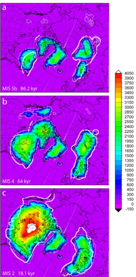
Fig. 5. Modeled ice sheet thickness for MIS 5b (a), MIS 4 (b) and
MIS 2 (c). Geological and geomorphological constraints from Fig. 3 are shown as thick white lines.
The goodness of fit in this procedure was judged through direct visual comparison of model-produced ice sheet out-lines and geological constraints. An alternative approach would have been to use goodness-of-fit metrics which could then be used as the basis for an automated search algorithm. However, all meaningful metrics we know of require com-plete targets that can be fully numerically described. For sev-eral of our targets only incomplete outlines and first-order dome patterns are available. These incomplete outlines
rep-resent real and useful constraining data, but do not allow the use of metrics for e.g. ice sheet area or center of grav-ity. We regard the present approach as expedient and ap-propriate for our ultimate goal, which is to provide reason-able first-order large-scale ice sheet reconstructions for use in climate modeling.
5 Results
5.1 Fit to the constraints
Figure 5 shows ice thickness in relation to the constraints, and Fig. 6 shows ice elevations. The main deviations from a “perfect” fit to the geological constraints for stage 5b are the following. There is too little ice in Newfoundland, making the Quebec Dome shorter in the NW–SE direction than the constraints indicate, and too much ice on the western flank of the Quebec Dome. The overall size of the Quebec Dome is in line with the constraints. The model slightly undershoots the minimum size for the proto-Keewatin Dome. In Eurasia, there is too little ice in southern Norway, and the Scandina-vian Ice Sheet reaches a somewhat larger easterly extent than indicated by the constraints. The Barents-Kara Dome is well centered within the constraints but slightly too small, partic-ularly in the sector of the Putorana Plateau. In line with the situation in North America, over- and undershoots of the ice margin largely cancel out.
For stage 4, the fit is in general very good. The only sig-nificant deviations from the constraints are the somewhat too small ice extent in the Canadian Maritimes, a slightly too small extent of the proto-Keewatin Dome, and some excess ice in the easternmost part of the Eurasian Ice Sheet. The model generates a plausible Cordilleran ice sheet with re-stricted extent and an easterly located ice divide.
5.2 Paleotopographic evolution
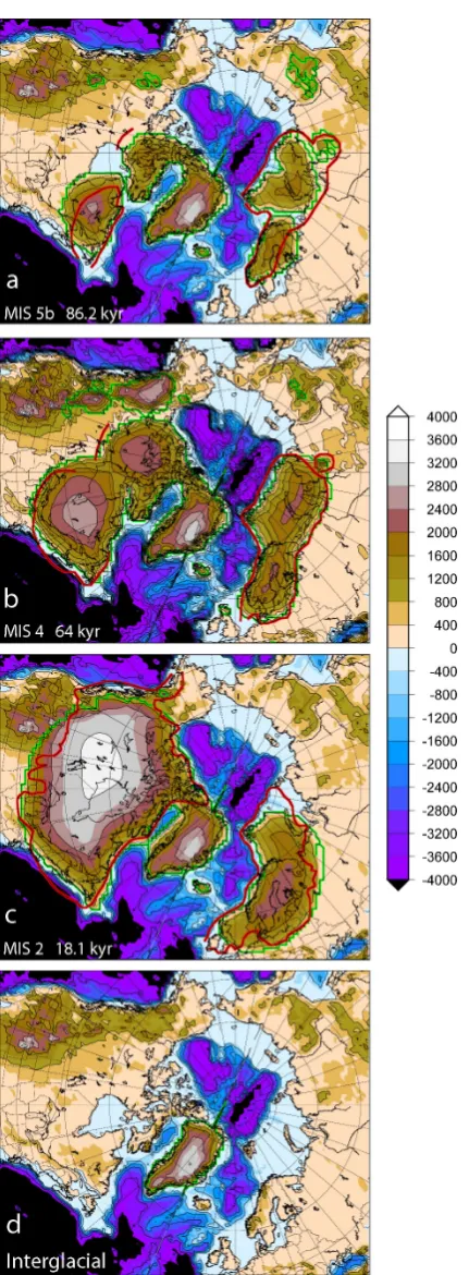
In the paleotopographic plots (Fig. 6) we see that the inter-glacial topography is characterized by two major highlands of a size large enough to significantly affect atmospheric circulation; Rocky Mountains–Coast Range and Greenland. In contrast to the situation in North America and Eurasia, glaciation south of 60◦N is impossible in Greenland. Dur-ing stage 5b (Fig. 6a), emergDur-ing ice sheets constitute four additional highlands large enough to potentially influence at-mospheric circulation. These are arranged in pairs in close proximity to each other, the Barents-Kara Ice Sheet and the Scandinavian Ice Sheet in Eurasia, and the Quebec and cen-tral Arctic domes in North America. These pairs constitute two highlands, 3500 and 3000 km long, respectively, each with only a minor gap in the central parts.
Fig. 6. Terrain topography and modeled ice sheet surface
topogra-phy for MIS 5b (a), MIS 4 (b), and MIS 2 (c). (d) Holocene topog-raphy shown for reference.
between the Rocky Mountains and the two ice sheets on the easternmost part of the continent.
By stage 4 (Fig. 6b), the number and location of ice sheets is still the same as during stage 5b, but the Quebec Dome has grown radically, constituting the largest topographic feature in the Northern Hemisphere with the exception of the Tibetan Plateau. The North American and Eurasian ice sheets are by this stage both over 3500 km long, each with a high saddle connecting two domes. The separation between the North American Ice Sheet and the Rocky Mountains has shrunk to few hundred kilometers in the north, and approximately 1500 km further south.
The time separation between stage 4 and the LGM is large, more than 40 kyr, and there is conflicting evidence (Ukko-nen, 2003; Helmens and Engels, 2010; Wohlfarth, 2010) re-garding the ice extent in both Eurasia and North America during stage 3. Our model indicates a significant shrinkage of ice in Eurasia, but a slow growth in North America. In stage 2 (Fig. 7c) the total ice sheet size and elevation in Eura-sia is approximately similar to stage 4, but its footprint has moved 700 km to the southwest. The North American evolu-tion leading into stage 2 is far more dramatic. Here, the two eastern and northern domes have merged with the Cordilleran Ice Sheet, to form a unified Laurentide and Cordilleran ice sheet reaching from coast to coast. There is no longer a midcontinent gap, and consequently the number of obstacles across the westerlies is down to three, although one of them has a very large east–west extent.
5.3 Evolution of mass
A surprising observation regarding the evolution of mass for Eurasian and North American ice sheets is the contrast be-tween the behaviors of the two ice sheets. The ice volume curve (Fig. 3b) shows ice volume variation until approx-imately 70 kyr as being in concert on the two continents, and being of comparable magnitude. However, during stage 4 and stage 2 the volume build-up is far more dramatic in North America than in Eurasia. During stage 5b ice volume in North America is larger than in Europe by a factor of 1.3. During stage 4 this number increases to 2, and by stage 2 North America has four times the Eurasian amount of ice.
6 Discussion
6.1 Forcing of the model
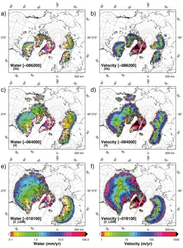
Fig. 7. Water production through basal melting (in mm yr−1) for MIS 5b (a), MIS 4 (c), and MIS 2 (e). Column-averaged velocities (m yr−1) for MIS 5b (b), MIS 4 (d), and MIS 2 (f).
the British Isles) is a common deficiency when simple north-pole-centered mass balance schemes are employed, even when present-day zonal climate anomalies are built in (Abe-Ouchi et al., 2007). Still, in order to tune the ice sheet model to the available constraints, we have chosen the first approach because it allows the main zonal climatic asymmetries of the high latitudes to be modeled in a simple way by shift-ing the “climatic pole”. No similar straightforward spatial-tuning possibility exists for fixed climate fields, and it is
model results. In combination with atmospheric circulation modeling, our reconstructions can be used to examine the zonal climate anomalies that arise from interactions between the ice sheet topography and the atmospheric circulation (Roe and Lindzén, 2001; Liakka and Nilsson, 2010). Such studies should provide additional physical information, help-ing to refine the present first-order reconstructions of the ice sheet topography.
When comparing with the recent ensemble modeling study by Stokes et al. (2012) we notice that they agree on a first-order pattern of ice build-up on the northeastern continental rim, but that the two models differ regarding the presence or absence of a robust Quebec Dome during stage 5b. The Stokes et al. model also indicates an early (MIS 4) full con-fluence between the Cordilleran and Laurentide ice sheets and complete incursion of the Canadian prairies already at that time. The volume evolution of the studies shows con-siderable similarity, both agreeing on small and comparable ice sheet volumes through stage 5 and a radical build-up of mass during stage 4. However, they differ in that the Stokes et al. (2012) study shows more dramatic stadial-interstadial swings in ice volume. This may be related to their inclusion of surficial and extramarginal (pro-glacial lakes) hydrology in their model, the effect of which will be that calving in such lakes is an additional fast process for ablation during interstadials.
6.2 Overall glaciation patterns during the three stadials 5b, 4 and 2
When comparing the evolution of the Eurasian and North American ice sheets through the three stages 5b, 4 and 2, some striking patterns emerge. In northeastern Eurasia, it ap-pears that the ice sheet extent became successively smaller through the three stages, closely mimicking the diminishing amplitude of the corresponding insolation minima. In con-trast, the southwestern extent of the ice sheet increased suc-cessively through these three events. Hence, the whole foot-print of the ice sheet moved to the southwest. In contrast to the North American situation, a clear highland center of glaciation existed in the Scandinavian mountains throughout the glaciation cycle. Only during the LGM did the center of mass move eastwards, to eastern Sweden and the Baltic de-pression (Ljungner, 1949; Kleman et al., 1997).
The evolution in North America was quite different. Ice cover during stage 5b was likely to have already been estab-lished over the entire NE continental rim, from Newfound-land to the Queen Elizabeth IsNewfound-lands. The evolution there-after was mainly an expansion over the interior continental areas, rapid in the east with a full expansion of the Que-bec Dome to the vicinity of the LGM margin during stage 4. The expansion in the west is poorly constrained but was apparently much slower. The southern and central prairies were not infilled before stage 2. This pattern indicates that build-up of the western part of the Laurentide Ice Sheet
was precipitation-limited because of poor access of moist air masses to the area. The range in glaciated area and volume through these three stages is much larger in North America than in Eurasia. We note that the volume differences in Eura-sia are modest between stages 5b, 4 and 2, and that North America differs radically in response by very rapid increases towards stage 4 and stage 2, respectively.
We speculate that Fennoscandian glaciation, due to the presence of a long high-precipitation backbone which deter-mined the basic build-up pattern, followed the same general growth and decay pattern during all glacial cycles. Such sta-bility in glaciation pattern cannot be expected to have pre-vailed in North America. Due to the lack of a similar high-land backbone, the growing ice sheets rapidly developed dis-persal centers far removed from any topographic highlands. Hence, renewed ice growth after interstadials with incom-plete deglaciation could occur on a “topography” that radi-cally differed from the fully ice-free interglacial one. Hence, North American glaciation can be expected to have been much more prone to hysteresis effects than glaciation in Eurasia. This inference is to some extent confirmed by geo-logical evidence for ice sheet configurations radically differ-ent from any that seem to have existed during the last glacial cycle. Magnetostratigraphy of tills indicate early Quaternary Laurentide ice sheets with a full N–S extent but with re-stricted ice cover on the prairies as well as in the Atlantic provinces (Barendregt and Irving, 1998). The climatology that would produce such a mid-continent glaciation pattern is to our knowledge completely unexplored.
6.3 Reconstructed ice sheet elevations
We expect reconstructions of ice elevations to be more accu-rate during build-up stages than for LGM and later stages, because during build-up phases the fraction of frozen bed was higher (Stokes et al., 2012), isostatic depression modest and delayed, and ice mostly terrestrial as opposed to marine-based. However, no known geological evidence allows direct evaluation of interior ice sheet elevations. An assessment of model performance in this respect therefore comes down to evaluation of the soundness of the model and the parameter settings and assumptions employed. Because of the relatively coarse grid we used, the model ice streams are rather broad and diffuse, and smaller topographically controlled streams may not be manifest at all, which may lead to an overesti-mate of marginal ice thickness, the effect of which will lessen inland. Figure 7 includes basal melt rates for the 3 modeled stages, as well as the resulting velocity field. Many major known ice streams are apparent here, albeit broader and less concentrated in their flow than they would be with higher-resolution topography.
coastal rim. The same holds true for both proto-Laurentide ice sheets in North America. In the model neither of them is as high as the Greenland Ice Sheet. Only at the LGM does our model show a Laurentide Ice Sheet that reaches above 3200 m, with one central dome. We will not here reiterate the long-standing debate over mono-dome vs. multi-dome con-figuration, but refer to Kleman et al. (2010) for a discussion on this topic. Our model shows an initially two-domed ice sheet that develops into a mono-dome during the LGM. The split into a deglacial two-dome configuration is well docu-mented (Dyke et al., 2002). Hence, there is good evidence that the basic ice sheet topology changed during the glacial cycle, but the geological evidence is relatively powerless for discriminating between e.g. a high or a low saddle connecting the Quebec and Keewatin domes. Our model underestimates the LGM ice sheet extent in westernmost Canada, probably due to the long poleward distance in the model domain when the climatic pole is located in east central Greenland. In terms of area and volume this is approximately compensated by an overshoot of the ice margin on the western prairies. The LGM ice sheet reaches the geologically documented maxi-mum southerly extent.
The total modeled Northern Hemisphere ice volume reaches approximately 100 m sea-level equivalent at LGM, thus allowing for a 20 m contribution from the Southern Hemisphere. Assuming the constraining footprints of North-ern Hemisphere ice sheets to be correct, this constitutes a test on the modeled ice sheet height; any serious over- or under-shoot of heights would have shown show up as implausible LGM volumes.
7 Conclusions
Using geologically and geomorphologically constrained nu-merical ice sheet modeling we have explored the evolution of Northern Hemisphere ice sheets during the build-up phase of the last glacial cycle. The model credibly reproduces the first-order pattern of size and location of geologically indi-cated ice sheets during marine isotope stages (MIS) 5b and 4. The differences in ice margin outline between constraints and model are considered to be small enough that they will not adversely affect the intended use; atmospheric circulation modeling based on the two paleotopographical data sets, for stages 5b and 4 respectively.
The results show that from an interglacial state of two north–south-oriented obstacles to atmospheric circu-lation (Rocky Mountains and Greenland), by MIS 5b the emergence of combined Quebec–central Arctic and Scandinavian–Barents-Kara ice sheets had effectively in-creased the number of such highland obstacles to four. This basic pattern was established already during stage 5d. This number of ice sheets remained constant through MIS 4, with the most significant change being a large increase in area and southerly extent of the Quebec Dome. By MIS 2, the
con-fluence of the Laurentide and Cordilleran ice sheets had re-duced the number to three, albeit one of them with a very large east–west extent.
The controls on growth pattern appear to have been dis-tinctively dissimilar in Eurasia and North America. In Eura-sia, the whole footprint of the ice sheet over the three stages moved in a southwesterly direction, towards the main precip-itation source, with only modest and short-lived expansion into the continental interior at the LGM. In North Amer-ica, the entire northeastern continental rim was glaciated early on, and expansion thereafter was by successive infill-ing of the continental interior, more rapid in the east than in the west.
Acknowledgements. This work was supported by a grant from the
Swedish Research Council to Johan Kleman, and by a Linéaus grant from the Swedish Research Council and FORMAS to The Bolin Centre of Stockholm University.
Edited by: V. Rath
References
Abe-Ouchi, A., Segawa, T., and Saito, F.: Climatic Conditions for modelling the Northern Hemisphere ice sheets throughout the ice age cycle, Clim. Past, 3, 423–438, doi:10.5194/cp-3-423-2007, 2007.
Álvarez-Solas, J., Montoya, M., Ritz, C., Ramstein, G., Charbit, S., Dumas, C., Nisancioglu, K., Dokken, T., and Ganopolski, A.: Heinrich event 1: an example of dynamical ice-sheet reaction to oceanic changes, Clim. Past, 7, 1297–1306, doi:10.5194/cp-7-1297-2011, 2011.
Barendregt, R. W. and Irving, E.: Changes in the extent of North American ice sheets during the late Cenozoic, Can. J. Earth Sci., 35, 504–509, 1998.
Bintanja, R., van de Wal, R. S. W., and Oerlemans, J.: Global ice volume variations through the last glacial cycle simulated by a 3-D ice-dynamical model, Quaternary Int., 95–96, 11–23, 2002. Bintanja, R. and van de Wal, R. S. W.,: North American ice-sheet dynamics and the onset of 100,000-year glacial cycles, Nature, 454, 869–872, 2008
Bonelli, S., Charbit, S., Kageyama, M., Woillez, M.-N., Ramstein, G., Dumas, C., and Quiquet, A.: Investigating the evolution of major Northern Hemisphere ice sheets during the last glacial-interglacial cycle, Clim. Past, 5, 329–345, doi:10.5194/cp-5-329-2009, 2009.
Boulton, G. S. and Clark, C. D.: A highly mobile Laurentide ice sheet revealed by satellite images of glacial lineations, Nature, 346, 813–817, 1990.
Charbit, S., Ritz, C., Philippon, G., Peyaud, V., and Kageyama, M.: Numerical reconstructions of the Northern Hemisphere ice sheets through the last glacial-interglacial cycle, Clim. Past, 3, 15–37, doi:10.5194/cp-3-15-2007, 2007.
Clague, J. J.: Quaternary geology of the Canadian Cordillera, in: Quaternary Geology of Canada and Greenland, edited by: Fulton, R. J., Geological Society of America, Boulder, CO, 15–95, 1989. Clark, P. U., Clague, J. J., Curry, B. B., Dreimanis, A., Hicock, S. R., Miller, G. H., Berger, G. W., Eyles, N., Lamothe, M., Miller, B. B., Mott, R. J., Oldale, R. N., Stea, R. R., Szabo, J. P., Thor-leifson, L. H., and Vincent, J.-S.: Initiation and development of the Laurentide and Cor-dilleran Ice Sheets following the last in-terglaciation, Quaternary Sci. Rev., 12, 79–114, 1993.
Clark, P. U., Licciardi, J. M., MacAyeal, D. R., and Jenson, J. W.: Numerical reconstruction of a soft-bedded Laurentide during the Last Glacial Maximum, Geology, 24, 679–682, 1996.
Cook, K. H. and Held, I. M.: Stationary Waves of the Ice Age Cli-mate, J. CliCli-mate, 1, 807–819, 1988.
Denton, G. H. and Hughes, T. J. (Eds.): The Last Great Ice Sheets, Wiley-Interscience, New York, 484 pp., 1981.
Dredge, L. A. and Thorleifson, H.: The Middle Wisconsinan history of the Laurentide Ice Sheet, Géographie Physique et Quaternaire, 41, 215–235, 1987.
Dyke, A. S., Andrews, J. T., Clark, P. U., England, J. H., Miller, G. H., Shaw, J., and Veillette, J. J.: The Laurentide and Innuitian ice sheets during the last glacial maximum, Quaternary Sci. Rev., 21, 9–31, 2002.
Ehlers, J. and Gibbard, P. L.: The extent and chronology of glacia-tions, Quaternary Sci. Rev., 22, 15–17, 2003.
England, J., Atkinson, N., Bednarski, J., Dyke, A. S., Hodgson, D. A., and Ó Cofaigh, C.: The Innuitian Ice Sheet: configuration, dynamics and chronology, Quaternary Sci. Rev., 25, 689–703, 2006.
EPICA Community Members: One-to-one coupling of glacial cli-mate variability in Greenland and Antarctica, Nature, 444, 195– 198, 2006.
Fastook, J. L. and Chapman, J.: A map plane finite-element model: Three modeling experiments, J. Glaciol., 35, 48–52, 1989. Fastook, J. L.: The finite-element method for solving conservation
equations in glaciology, Comput. Sci. Eng., 1, 55–67, 1993. Fastook, J. L. and Prentice, M.: A finite-element model for
Antarc-tica; Sensitivity test for meteorological mass-balance relation-ship, J. Glaciol., 40, 167–175, 1994.
Gregoire, L. J., Payne, A. J., and Valdes, P. J.: Deglacial rapid sea-level rises caused by ice-sheet saddle collapses, Nature, 487, 219–222, 2012.
Held, I. M., Ting, M., and Wang, H.: Northern Winter Stationary Waves: Theory and Modeling, J. Climate, 15–16, 2125–2144, 2002.
Helmens, K. and Engels, S.: Ice-free conditions in eastern Fennoscandia during early Marine Isotope Stage 3: lacustrine records, Quaternary Sci. Rev., 39, 399–409, 2010.
Holmlund, P. and Fastook, J. L.: A time dependent glaciological model of the Weichselian ice sheet, Quaternary Int., 27, 53–58, 1995.
Huybrechts, P.: A 3-D model for the Antarctic Ice Sheet: A sensi-tivity study on the glacial-interglacial contrast, Clim. Dynam., 5, 79–92, 1990.
Huybrechts, P. and T’siobbel, S.: Thermomechanical modelling of Northern Hemisphere ice sheets with a two-level mass-balance parameterization, Ann. Glaciol., 21, 111–116, 1995.
Imbrie, J., Harys, J. D., Martinson, D. G., McIntyre, A., Mix, A. C., Morley, J. J., Pisias, N. G., Prell, W. I., and Shackleton, N. J.: The orbital theory of Pleistocene climate: Support from revised chronology of the marineδ18O record, in: Milankovitch and Cli-mate, edited by: Berger, A. I., Imbrie, J., Hays, J., Kukla, G., and Saltzman, B., Part 1. Reidel, Dordrecht, 269–305, 1984. Imbrie, J. Z., Imbrie-Moore, A., and Lisiecki, L. E.: A phase-space
model for Pleistocene ice volume, Earth Planet. Sci. Lett., 307, 94–102, 2011.
Johnsen, S. J., Clausen, H. B., Dansgaard, W., Gundestrup, N. S., Hammer, C. U., Andersen, U., Andersen, K. K., Hvidberg, C. S., Dahl-Jensen, D., Steffensen, J. P., Shoji, H., Sveinbjörnsdót-tir, A. E., White, J. W. C., Jouzel, J., and Fisher, D.: Theδ18O record along the Greenland Ice Core Project deep ice core and the problem of possible Eemian climatic instability, J. Geophys. Res., 102, 26397–26410, 1997.
Johnson, J. and Fastook, J. L.: Northern Hemisphere glaciation and its sensitivity to basal melt water, Quaternary Int., 95–96, 65–74, 2002.
Kageyama, M., Valdes, P. J., Ramstein, G., Hewitt, C., and Wyputta, U.: Northern Hemisphere Storm Tracks in Present Day and Last Glacial Maximum Climate Simulations: A comparison of the Eu-ropean PMIP Models, J. Climate, 12, 742–760, 1999.
Kleman, J., Hättestrand, C., Borgström, I., and Stroeven, A. P.: Fennoscandian paleoglaciology reconstructed using a glacial ge-ological inversion model, J. Glaciol., 43, 283–299, 1997. Kleman, J., Jansson, K. N., De Angelis, H., Stroeven, A. P.,
Hättes-trand, C., Alm, G., and Glasser, N. F.: North American Ice Sheet build-up during the last glacial cycle 115–21 kyr, Quaternary Sci. Rev., 29, 2036–2051, 2010.
Kleman, J., Fastook, J., and Stroeven, A.: Geologically and ge-omopholocally constrainednumerical model of Laurentide Ice Sheet inception and build-up, Quaternary Int., 95–96, 87–98, 2002.
Kleman, J. and Hättestrand, C.: Frozen-based Fennoscandian and Laurentide ice sheets during the last glacial maximum, Nature, 402, 63–66, 1999.
Lambeck, K., Esat, T. M., and Potter, E. M.: Links between climate ansd sea-levels for the past three million years, Nature, 419, 199– 206, 2002.
Lambeck, K., Purcell, A., Funder, S., Kjær, K. H., Larsen, E., and Möller, P.: Constraints on the Late Saalian to early Middle We-ichselian ice sheet of Eurasia from field data and rebound mod-elling, Boreas, 35, 539–575, 2006.
Landwehr, J. M., Coplen, T. B., Ludwig, K. R., Winograd, I. J., and Riggs, A.: Data from Devils Hole Core DH-11, USGS Open File Rep. 97–792, USGS, Washington D.C., 1997.
Langen, P. L. and Vinther, B. M.: Response in atmospheric circula-tion and sources of Greenland precipitacircula-tion to glacial boundary conditions, Clim. Dynam., 32, 1035–1054, 2009.
Liakka, J., Nilsson, J., and Löfverström, M.: Interactions be-tween stationary waves and ice sheets: linear versus non-linear atmospheric response, Clim. Dynam., 37, 531–553, doi:10.1007/s00382-011-1004-6, 2011.
Lisiecki, L. E. and Raymo, M. E.: A Pliocene-Pleistocene stack of 57 globally distributed bethicδ18O records, Paleoceanography, 20, doi:10.1029/2004PA001071, 2005.
Ljungner, E.: East-west balance of the Quaternary ice caps in Patag-onia and Scandinavia. Buletin of the Geological Institute, Upp-sala, 33, 1–96, 1949.
Lourens, L. J., Becker, J., Bintanja, R., Hilgen, F. J., Tuenter, E., van de Wal, R. S. W., and Ziegler, M.: Linear and non-linear response of the late Neogene glacial cycles to obliquity forcing and impli-cations for the Milankovitch theory, Quaternary Sci. Rev., 29, 352–365, 2010.
Lundqvist, J.: Glacial history of Sweden, in: Quaternary glaciations – Extent and Chronology, edited by: Ehlers, J. and Gibbard, P. L., Vol. 1. Europe, Elsevier, Amsterdam, 2004.
Ma, Y., Gagliardini, O., Ritz, C., Gillet-Chaulet, F., Durand, G., and Montagnat, M.: Enhancement factors for grounded ice and ice shelves inferred from an anisotropic ice-flow model, J. Glaciol., 56, 805–812, 2010.
Manabe, S. and Broccoli, A. J.: The influence of continental ice sheets on the climate of an ice age, J. Geophys. Res., 90, 2167– 2190, 1985.
Mangerud, J.: Ice sheet limits in Norway and on the Norwegian con-tinental shelf, in: Quaternary glaciations – Extent and Chronol-ogy, edited by: Ehlers, J. and Gibbard, P. L., Vol.. 1, Europe, Elsevier, Amsterdam, 2004.
Marshall, S. J., Tarasov, L., Clarke, G. K. C., and Peltier, W. R.: Glaciological reconstruction of the Laurentide Ice Sheet: Phys-ical processes and modelling challenges, Can. J. Earth Sci., 37, 769–793, 2000.
McMartin, I. and Henderson, P. J.: Evidence from Keewatin (central Nunavut) for paleo-ice divide migration, Géographie Physique et Quaternaire, 58, 163–186, 2004.
Otieno, F. O. and Bromwich, D. H.: Contribution of Atmospheric Circulation to Inception of the Laurentide Ice Sheet at 116 kyr BP, J. Climate, 22, 39–57, 2009.
Otto-Bliesner, B. L., Brady, E. C., Clauzet, G., Tomas, R., Levis, S., and Kothavala, Z.: Last Glacial Maximum and Holocene Climate in CCSM3, J. Climate, 19, 2526–2544, 2006.
Paterson, W. S. B.: The physics of glaciers, 3rd Edn., Pergamon, Oxford, 1994.
Peltier, W. R.: Global Glacial Isostasy and the Surface of Ice-Age earth: The ICE-5G (VM2) Model and GRACE, Ann. Rev. Earth Planet. Sci., 32, 111–149, 2004.
Petit, J. R., Jouzel, J., Raynaud, D., Barkov, N. I., Barnola, J.-M., Basile, I., Benders, M., Chappellaz, J., Davis, M., Delayque, G., Delmotte, M., Kotlyakov, V. M., Legrand, M., Lipenkov, V. Y., Lorius, C., Pépin, L., Ritz, C., Saltzman, E., and Stievenard, M.: Climate and atmospheric history of the past 420,000 years from the Vostok ice core, Antarctica, Nature 399, 429–436, 1999.
Roe, G. H. and Lindzén, R. S.: The mutual Interaction between Continental-Scale Ice Sheets and Atmospheric Stationary Waves, J. Climate, 14, 1450–1465, 2001.
Stea, R. R.: The Appalachian glacier Complex in Maritime Canada, in Quaternary Glaciations – Extent and Chronology, Part II: North America, edited by: Ehlers, J. and Gibbard, P. L., Elsevier, Amsterdam, 213–232, 2004.
Stokes, C. R., Tarasov, L., and Dyke, A. S.: Dynamics of the North American Ice Sheet Complex during its inception and build-up to the last glacial maximum, Quaternary Sci. Rev., 50, 86–104, 2012.
Stumpf, A. J., Broster, B. E., and Levson, V. M.: Multiphase flow of the Late Wisconsinan Cordilleran ice sheet in western Canada, Geol. Soc. Am. Bull., 112, 1850–1863, 2000.
Svendsen, J. I., Alexanderson, H., Astakhov, V. I., Demidov, I., Dowdeswell, J. A., Funder, S., Gataullin, V., Henriksen, M., Hjort, C., Houmark-Nielsen, M., Hubberten, H. W., Ingolfs-son, O., JakobsIngolfs-son, M., Kjaer, K. H., Larsen, E., Lokrantz, H., Lunkka, J. P. Lyså, A., Mangerud, J., Matiouchkov, A., Murray, A., Moller, P., Niessen, F., Nikolskaya, O., Polyak, L., Saarnisto, M., Siegert, C., Siegert, M. J., Spielhagen, R. F., and Stein, R.: Late Quaternary ice sheet history of northern Eurasia, Quater-nary Sci. Rev., 23, 1229–1271, 2004.
Svensson, A., Bigler, M., Blunier, T., Clausen, H. B., Dahl-Jensen, D., Fischer, H., Fujita, S., Goto-Azuma, K., Johnsen, S. J., Kawa-mura, K., Kipfstuhl, S., Kohno, M., Parrenin, F., Popp, T., Ras-mussen, S. O., Schwander, J., Seierstad, I., Severi, M., Stef-fensen, J. P., Udisti, R., Uemura, R., Vallelonga, P., Vinther, B. M., Wegner, A., Wilhelms, F., and Winstrup, M.: Direct linking of Greenland and Antarctic ice cores at the Toba eruption (74 ka BP), Clim. Past, 9, 749–766, doi:10.5194/cp-9-749-2013, 2013. Tarasov, L. and Peltier, W. R.: A geophysically constrained large
ensemble analysis of the deglacial history of the North American ice-sheet complex, Quaternary Sci. Rev., 23, 359–388, 2004. Ukkonen, P., Arppe, L., Houmark-Nielsen, M., Kjaer, K. H., and
Karhu, J. A.: MIS 3 Mammoth remains from Sweden – implica-tions for faunal history and paleoclimate and glaciation chronol-ogy, Quaternary Sci. Rev., 26, 3081–3098, 2003.
Weertman, J.: Deformation of floating ice shelves, J. Glaciol., 3, 38–42, 1957.
Weertman, J.: The theory of glacier sliding, J. Glaciol., 5, 287–303, 1964.
Weertman, J.: Water lubrication mechanism of glacier surges, Can. J. Earth Sci., 6, 929–942, 1969.
Weertman, J. and Birchfield, G. E.: Subglacial water flow under ice streams and West Anterctic ice sheet stability, Ann. Glaciol., 3, 316–320, 1982.
Winsborrow, M., Clark, C., and Stokes, C.: Ice streams of the Lau-rentide ice sheet, Geìographie Physique et Quaternaire, 58, 269– 280, 2004.