Salman Abbas
Department of Mathematics,
COMSATS University Islamabad, Wah Capmus, Pakistan [email protected]
Gamze Ozal
Department of Statistics
Hacettepe University, Ankara, Turkey [email protected]
Saman Hanif Shahbaz
Department of Statistics
King Abdulaziz University, Jeddah, Kingdom of Saudi Arabia [email protected]
Muhammad Qaiser Shahbaz
Department of Statistics
King Abdulaziz University, Jeddah, Kingdom of Saudi Arabia [email protected]
Abstract
In this article, we present a new generalization of weighted Weibull distribution using Topp Leone family of distributions. We have studied some statistical properties of the proposed distribution including quantile function, moment generating function, probability generating function, raw mo-ments, incomplete momo-ments, probability, weighted momo-ments, Rayeni and q−th entropy. We have obtained numerical values of the various measures to see the effect of model parameters. Distribu-tion of order statistics for the proposed model has also been obtained. The estimaDistribu-tion of the model parameters has been done by using maximum likelihood method. The effectiveness of proposed model is analyzed by means of a real data sets. Finally, some concluding remarks are given.
Keywords: Weighted Weibull, Topp Leone family, Order Statistics, Entropy
1. Introduction
In some situations, it is found that the classical distributions are not suitable for the data sets related to the field of engineering, financial, biomedical, and environmental sciences. The extension of classical models is, therefore, continually needed to obtain suitable model for applications in these areas. Researchers have obtained several ex-tended models for use in these situations but still the room is available to obtain new models with much wider applicability.
Weibul-l distribution by Zhang and Xie (2011), The Topp-Leone Generated WeibuWeibul-lWeibul-l dis-tribution by Aryal et al. (2016), Generalized weibull disdis-tributions by Lai, (2014), The Kumaraswamy-transmuted exponentiated modified Weibull distribution by Al-Babtain et al. (2017), Generalized Flexible Weibull Distribution by Ahmad and Iqbal (2017), A reduced new modified Weibull distribution by Almalki (2018), and the transmuted exponentiated additive Weibull distribution by Nofal et al. Nofal et al.. Nasiru (2015) proposed a new Weighted Weibull (WW) distribution and discussed its statistical properties using Azzalani’s family of weighted distributions by Azzalini (1985). The density (pdf) and distribution function (cdf) of the WW distribution are given by
f(x) = (1 +λγ)αγxγ−1e−αxγ(1+λγ); x, α, λ >0, (1)
and
F(x) = 1−e−αxγ(1+λγ) x, α, λ >0, (2)
where,α is a scale parameter and λ and γ are shape parameters. The corresponding survival function of the WW distribution is given by
¯
F(x) =e−αxγ(1+λγ). (3)
Note that the WW distribution reduces to Weibull distribution for λ= 0 .
Topp-Leone family of distributions is proposed by Al-Shomrani et al. (2016). The cdf of the proposed family is given by
FT L−G(t) = [G(t)]b[2−G(t)]b = [1−( ¯G(t))2]b :, x<, b > 0 (4)
and the corresponding pdf is obtained as
fT L−R(t) = 2bg(t) ¯G(t)[1−( ¯G(t))2]b−1, b >0. (5)
where g(t) =G0(t) and ¯G(t) = 1−G(t).
In this paper a new generalization of the WW distribution, the Topp Leone Weight-ed Weibull (TLWW) distribution, is obtainWeight-ed. The aim of this generalization is to provide a flexible extension of the WW distribution which can be used in much wider situations.
The paper is organized as follows: The pdf and cdf of the proposed model is intro-duced and several mathematical characteristics are studied in Section 2. Distribution of the order statistics is obtained in Sec. 4. Estimation of the model parameters are done in Sec. 5. The influence of the estimators are evaluated in Sec. 6. The validity of prosed model is on real data is presented in Sec. 7. Some concluding remarks are given in Sec. 8.
2. Topp-Leone Weighted Weibull Distribution and its Properties
The cdf of the TLWW distribution is obtained as
F(x) = [1−(e−αxγ(1+λγ))2]b = [1−e−2αxγ(1+λγ)]b, b >0. (6)
The density function is obtained by differentiating (6) and is given as
f(x) = 2bαγ(1 +λγ)xγ−1e−2αxγ(1+λγ)[1−e−2αxγ(1+λγ)]b−1, x, α, λ, γ, b >0, (7)
where, α, γ, b are shape parameters and λ is scale parameter. A random variable X havingpdf (7) is denoted asX ∼T LW W(α, λ, γ, b). The proposed model reduces to Topp Leone Weibull distribution forλ = 0. For λ= 0 andγ = 1, it reduces to Topp Leon Exponential distribution.
The reliability function (rf), which is also known as survival function, is the proba-bility of an item not failing prior to some time t. The rf of the TLWW distribution is obtained asR(x) = 1−H(x) and is given as
S(x) = 1−[1−e−2αxγ(1+λγ)]b.
The hazard rate function which is also known as, force of mortality in actuarial s-tatistics, Mill’s ratio in statistics and intensity function in extreme value theory are important characteristics in reliability theory, It is roughly explained as the condi-tional probability of failure, given it has survived to the time t. The hrf of random variable X is defined ash(x) = f(x)/R(x) and for TLWW distribution it is given as
h(x) = 2bαγ(1 +λ
γ)xγ−1e−2αxγ(1+λγ)
[1−e−2αxγ(1+λγ)
]b−1 1−[1−e−2αxγ(1+λγ)
]b .
The cumulative hrf of the TLWW distribution is given by
H(x) =−log|1−[1−e−2αxγ(1+λγ)]b|.
2.1 Limiting Behavior
The behaviors of the pdf, cdf and hrf of TLWW distribution are investigated when x→0 and x→ ∞. Therefore, lim
x→0f(x) and limx→∞f(x) are given in the following
lim
x→0f(x) = limx→0
2bαγ(1 +λγ)xγ−1e−2αxγ(1+λγ)[1−e−2αxγ(1+λγ)]b−1 = 0,
lim
x→∞f(x) = limx→∞
2bαγ(1 +λγ)xγ−1e−2αxγ(1+λγ)[1−e−2αxγ(1+λγ)]b−1 =∞
From above it is clear that the proposed model has a unique mode. The limiting behavior of cdf and hrf is given below
lim
x→0f(x) = limx→0
lim
x→∞f(x) = limx→∞
1−e−2αxγ(1+λγ)b = 1,
lim
x→0h(x) = limx→0
2bαγ(1 +λγ)xγ−1e−2αxγ(1+λγ)
[1−e−2αxγ(1+λγ)
]b−1 1−[1−e−2αxγ(1+λγ)
]
= 0,
lim
x→∞h(x) = limx→∞
2bαγ(1 +λγ)xγ−1e−2αxγ(1+λγ)
[1−e−2αxγ(1+λγ)
]b−1 1−[1−e−2αxγ(1+λγ)
]
= 0.
2.2 Shape
The distribution and density functions of the proposed model can be expressed in the form of exponentiated G-distribution. Prudnikov et al. (1986) presented a series representation and is given as
(1 +x)α =
∞
X
j=0
(1)jΓ(α+ 1)
j!Γ(α+ 1−j)x
j,
the distribution function of TLWW distribution is written as follow
F(x) =
∞
X
j=0
(−1)j Γ(b+ 1) j!Γ(b+ 1−j)(e
αxγ(1+λγ))2j.
The density of TLWW distribution can also be written in the form of exponentiated distributions and is given as
f(x) =
∞
X
j=0
(−1)j2Γ(b+ 1)
j!Γ(b−j) αγx
γ−1(1 +λγ) e−2αxγ(1+λγ)(j+1)
(8)
x
0 0.1 0.2 0.3 0.4 0.5 0.6 0.7 0.8 0.9 1
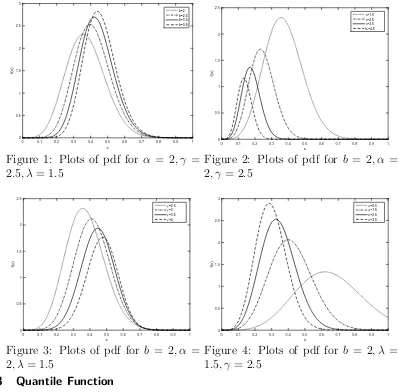
f(x) 0 0.5 1 1.5 2 2.5 3 b=2 b=2.5 b=3.0 b=3.5
Figure 1: Plots of pdf for α = 2, γ = 2.5, λ= 1.5
x
0 0.1 0.2 0.3 0.4 0.5 0.6 0.7 0.8 0.9 1
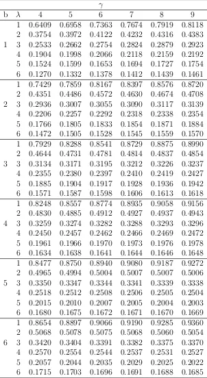
f(x) 0 0.5 1 1.5 2 2.5 λ=1.5 λ=2.5 λ=3.5
lλ=4.5
Figure 2: Plots of pdf for b = 2, α = 2, γ = 2.5
x
0 0.1 0.2 0.3 0.4 0.5 0.6 0.7 0.8 0.9 1
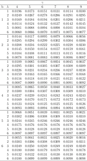
f(x) 0 0.5 1 1.5 2 2.5 γ=2.5 γ=3 γ=3.5 γ=4
Figure 3: Plots of pdf for b = 2, α = 2, λ= 1.5
x
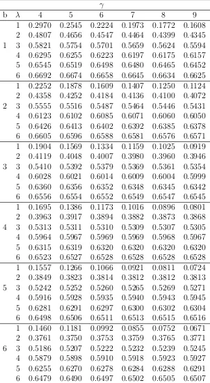
0 0.1 0.2 0.3 0.4 0.5 0.6 0.7 0.8 0.9 1
f(x) 0 0.5 1 1.5 2 2.5 3 α=0.5 α=1.5 α=2.5 α=3.5
Figure 4: Plots of pdf for b = 2, λ = 1.5, γ = 2.5
2.3 Quantile Function
The quantile function of the TLWW distribution is obtained as Q(u) = F−1(u) and given as
Q(u) = − ln{1−u 1
b}
2α(1 +λγ)
!γ1
, f or α >0, u∈(0,1).
Median of the distribution can be obtained by replacing u = 0.5 in above equation. The quantile function is used to observe the effect of shape parameters on skewness and kurtosis. The Bowley’s measure of skewness (S) is given as
S = Q( 1
4) +Q( 3
4)−2Q( 1 2) Q(34)−Q(14)
and the Moors’s coefficient of kurtosis (K) is given as
K = Q( 7
8)−Q( 5
8) +Q( 3 8)−Q
2.4 Moments
The raw or non-central moment for any probability distribution is obtained by using
µ0q = Z ∞
−∞
xqdF(x).
Usingpdf of the TLWW distribution in (8), we obtain the raw moments of the TLWW distribution as
µ0q= Z ∞ 0 xq ∞ X j=0
(−1)j2Γ(b+ 1) j!Γ(b−j) αγx
γ−1(1 +λγ) e−2αxγ(1+λγ)(j+1)
.
From the transformation w = (j + 1)2αxγ(1 +λγ) and after some calculations, the q−th moment of TLWW distribution is obtained as
µ0q =
∞
X
j=0
bjΓ(1 +
q γ),
wherebj = (−1)jjΓ(!Γ(bb+1)−j)
1
j+1
γq+1 1 2α(1+λγ)
γq
. The coefficient of variation (CV),
co-efficient of skewness (CS), and coco-efficient of kurtosis (CK) of the TLWW distribution are obtained as follows
CV = r
µ2 µ1
−1,
CS = µ3−3µ2µ1+ 2µ 3 1 (µ2−µ1)32
,
CK = µ4−4µ3µ1+ 6µ2µ 2 1 (µ2−µ21)2
.
Now, the first incomplete moment is used to derive the mean deviation, Bonfer-roni, and Lorenz curves. These curves have great influences in economics, reliability, demography, insurance, and medicine. The incomplete moment of the TLWW distri-bution is obtained by using (7) and is given below.
ϕs(t) =
Z t 0 xs ∞ X j=0
(−1)j2Γ(b+ 1)
j!Γ(b−j) αγx
γ−1(1 +λγ) e−2αxγ(1+λγ)(j+1)
dx
Simplifying, the incomplete moments is given by
ϕs(t) =
∞
X
j=0
A∗j
γ(1 + s
γ)−γ(1 + s
γ),2α(1 +λ
γ)(j+ 1)
.
where A∗j = (−1)j Γ(b+1)
j!Γ(b−j)
1
j+1
γs+1 1 (2α(1+λγ))
γs .
µ01 − 2ϕ1(M), respectively, where µ01 = E(X), M = M edian(X) = Q(0.5), and F(µ01) is calculated from (7) and ϕ1(t) is the first incomplete moment given by (19) with s= 1.
These equations for ϕ1(t) can be used to obtain Bonferroni and Lorenz curves given probability π as B(π) = ϕ1πµ(q0)
1
and L(π) = ϕ1µ(0q) 1
, respectively, where µ01 = E(X) and q=Q(π) is quantile function of X atπ.
The (q, r)th probability weighted moment (PWM) of X is defined as
ρq,r =
Z ∞
−∞
xq[F(x)]rf(x)dx.
Using (5) and (6), we can write after some algebra,
[F(x)]rf(x) =
∞
X
j,m=0
a(j, m)h2j+1(x),
where
a(j, m) =
∞
X
j,m=0
(−1)j+m Γ(b+ 1)(rb+ 1) j!m!Γ(b−j)(rb+ 1−j)
and
h2j+1(x) = 2αγxγ−1(1 +λγ)e−2γx
γ(1+λγ)(2j+1)
,
After making transformation, the (q, r)th PWM of X can be expressed as
ρq,r(x) = a(j, m)
1 2j+ 1
γq+1 1 2α(1 +λγ)
qγ
Γ(1 + q γ).
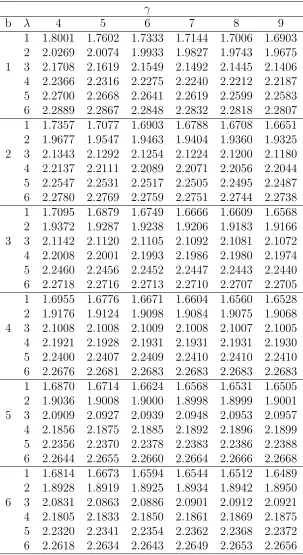
Table 1: Mean of TLWW distribution for α = 1 and various values of parameters
γ
b λ 4 5 6 7 8 9
Table 2: Variance of TLWW distribution for α = 1 and various values of parameters
γ
b λ 4 5 6 7 8 9
Table 3: Coefficient of skewness of the TLWW distribution for α = 1 and various values of parameters
γ
b λ 4 5 6 7 8 9
Table 4: Coefficient of kurtosis of TLWW distribution forα= 1and various values of parameters
γ
b λ 4 5 6 7 8 9
2.5 Moment and Probability Generating Function
LetX ∼T LW W(b, α, λ, γ), then the moment generating function ofX is denoted as MX(t) and is given as
MX(t) =
Z ∞
0
etxf(x)dx.
Using Taylor series and from (7), we have
MX(t) =
∞
X
i,j=0
ti
i
(−1)jΓ(b+ 1)
j!Γ(b−j)
1 j+ 1
γi+1
1 (2α(1 +λγ)
γi
Γ(1 + i
γ). (9)
Similarly, ifX ∼T LW W(b, α, λ, γ), then the probability generating function of X is denoted as P hiX(t) and is given as
ΦX(t) =
Z ∞
0
txf(x)dx.
Using
MX(t) =
∞
X
l=0
(lnt)lxl l!
we have,
ΦX(t) =
∞
X
l,j=0
(lnt)l
l!
)jΓ(b+ 1)
j!Γ(b−j)
1 j+ 1
γi+1 1 2α(1 +λγ)
γl
Γ(1 + l γ)
l
γ (10)
2.6 Order Statistics
The order statistics play an important role in the statistical theory. LetX1, X2, , , , , Xn
be a random samples from the TLWW distribution, then the density function of the i−th order statistics is given as
fi:n(x) =
∞
X
j=0
ψj(e−2αx
γ(1+λγ)
)m+1,
where
ψj =
n!
(i−1)!(n−i)!2αγ(1 +λ
γ)xγ−1
b(i+j)−1 X
m=0
n−1
j
b(i+j)−1 m
The pdf of the first order statistics can be obtained by usingi= 1 and the pdf ofnth order statistics can be defined by replacingi=n.
3. Entropy
The entropy is used to explain the existence of uncertainty in the random variables. Different method to measure the uncertainty in random variables are developed by researchers. Reyni’s entropy is obtained by using
Ip =
1 1−plog
Z ∞
−∞
f(x)pdx, p >0, p6= 0,
Now using Eq. (8), we have
Ip =
1 1−plog
Z ∞
−∞
∞ X
j=0
(−1)j2Γ(b+ 1)
j!Γ(b−j) αγx
γ−1(1 +λγ) e−2αxγ(1+λγ)(j+1)p
dx,
To obtained the expression of entropy, we assume z = 2αxγ(1 +λγ)(j+ 1), and after
simplification we have
Ip =
1 1−plog
κpjA∗Γ(p+ 1)
,
where
κ=
∞
X
j=0
(−1)j2Γ(b+ 1)
j!Γ(b−j) αγx
γ−1(1 +λγ)
A∗ =αp
1
2α(1 +λγ)(j + 1)
p
Next, the q−th entropy is define as
Hq =
1 q−1log
1−
Z ∞
−∞
f(x)qdx .
So, the q−th entropy for the TLWW distribution is given as
Hq =
1 q−1log
1−κqjA∗Γ(q+ 1)
,
where
κ=
∞
X
j=0
(−1)j2Γ(b+ 1)
j!Γ(b−j) αγx
γ−1(1 +λγ)
A∗ =αp
1
2α(1 +λγ)(j + 1)
4. Estimation
In this section, we have discussed estimation of the parameters of TLWW distribution. Let x1, x2, , , , xn be the random sample of size n from TLWW distribution. The log
likelihood function is, then, given as
L=nlog(2) +nlog(b) +nlog(α) +nlog(γ) +nlog(1 +λγ) + (γ−1)
n
X
i=0
xi
−2α(1 +λγ)
n
X
i=0
xγi + (b−1)
n
X
i=0
log(1−e−2αxγ(1+λγ)). (11)
The parameters are obtained by solving the nonlinear equations which are obtained by differentiating (11). The score vector components, say U(θ) = (dbdl,dαdl,dγdl,dλdl)T =
(Ub, Uα, Uγ, Uλ)T, are given as follows:
Uα =
n
α −2(1 +λ
γ)
n
X
i=0
xi+ (b−1) n
X
i=0
2xγi(1 +λγ)w i
1−wi
,
Ub =
n b +
n
X
i=0
log(1−wi),
Uγ =
n γ +
nλγlog(λ)
1 +λγ −2αλ
γlog(λ) n
X
i=0
xγi +
n
X
i=0
log(xi)−2α(1 +λ) n
X
i=0
xγi log(xi)
−(b−1)
n
X
i=0
wi(2xγα(1 +λ) log(xi)−2xγαλγlog(λ)
1−wi
,
Uλ =
nγλγ−1 1 +λγ 2αγλ
γ−1
n
X
i=0
xγi + (b−1)
n
X
i=0
2xγαγλγ−1w
i
1−wi
,
where wi = e−2αx
γ(1+λγ)
. The maximum likelihood estimate for the parameters are obtained by equating the above expressions equal to zero. For interval estimation of the parameters, we obtain the 4×4 observed information matrix given by
J(θ) = −
Jbb Jbα Jbγ Jbλ
Jαα Jαγ Jαλ
Jγγ Jγλ
Jλλ
5. Application
In this section, we show the performance of the proposed model with a real data set. We use the distributions in Table 5 to compare the existing distributions with the proposed distribution. The comparison has been done by fitting various models on
Table 5: Fitted Distributions and their Abbreviations
Distributions Abb Referrence Topp Leone Weighted Weibull TLWW Proposed
Kumaraswamy Weibull KwW (10)
Exponential Weibull ExW (9)
Exponentiated Weibull-Exponential ExpWEx (11) Marshall-Olkin exponential-Weibull MOEW (18)
Weighted Weibull WW (16)
real data sets and comparing the goodness of fit measures. In order to compare the fit of TLWW model with other models, we provide the values of the Akaike Information Criterion (AIC) and Consistent Akaike Information Criterion (CAIC).
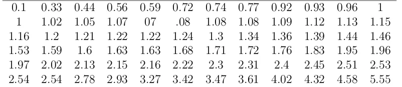
The data have been obtained from Bjerkedal by Bjerkedal et al. (1960) and represents the survival times (in days) of 72 guinea pigs infected with virulent tubercle bacilli. The data set is given in Table 6.
Table 6: Data for the survival time (9n days) of 72 guinea pigs infected with virulent tubercle bacilli
0.1 0.33 0.44 0.56 0.59 0.72 0.74 0.77 0.92 0.93 0.96 1 1 1.02 1.05 1.07 07 .08 1.08 1.08 1.09 1.12 1.13 1.15 1.16 1.2 1.21 1.22 1.22 1.24 1.3 1.34 1.36 1.39 1.44 1.46 1.53 1.59 1.6 1.63 1.63 1.68 1.71 1.72 1.76 1.83 1.95 1.96 1.97 2.02 2.13 2.15 2.16 2.22 2.3 2.31 2.4 2.45 2.51 2.53 2.54 2.54 2.78 2.93 3.27 3.42 3.47 3.61 4.02 4.32 4.58 5.55
In Table 7, the values of estimated parameters and the statistic are given. We can easily see that the proposed model provide smaller values of the computed statistics which indicate that it provides better fit than competing models.
Table 7: The MLEs and the values of AIC, CAIC and -2LL statistics
Model Parameters −2LL AIC CIAC
α λ γ λ
TLWW 0.078 2.037 1.157 3.055 205.62 213.62 214.217 KwW 1.655 0.232 1.355 1.615 207.311 215.311 215.908 ExW 1.617 0.311 1.2×10⁻⁸ - 208.034 214.034 214.387 ExpWEx 0.409 1.958 2.082 0.127 304.341 312.341 312.938 MOEW 0.091 0.012 2.940 - 245.993 251.993 252.346 WW 0.213 0.621 1.617 - 208.034 214.034 214.387
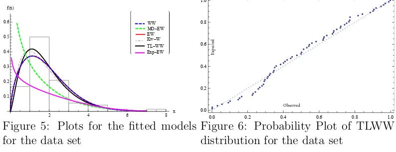
Figures 5 and 6 shows the plots for the fitted models and probability plot of the TLWW distribution, respectively.
WW
MO-EW EW Kw-W TL-WW Exp-EW
2 4 6 8
x 0.1
0.2 0.3 0.4 0.5 0.6 fHxL
Figure 5: Plots for the fitted models for the data set
0.0 0.2 0.4 0.6 0.8 1.0
0.0 0.2 0.4 0.6 0.8 1.0
Expected
Observed
Figure 6: Probability Plot of TLWW distribution for the data set
6. Conclusion
This paper presents the Topp Leone weighted Weibull distribution. We have obtained various properties for the proposed model; including, shape, moments, moment gen-erating function, probability gengen-erating moments, and reliability analysis. The effects of model parameters are discussed in terms of mean, variance, coefficient of skewness, and coefficient of kurtosis. The method of maximum likelihood is used for the estima-tion of the parameters. We study the data regarding the survival time of 72 Pigs (in days) for the evaluation of the proposed model in practical application. The results show that the proposed model is a better fit as compared with the available models for modeling of the used data.
References
1. Ahmad, Z. and Iqbal, B. (2017). Generalized flexible weibull extension distribution. Circulation in Computer, 2(4):68–75.
2. Al-Babtain, A., Fattah, A. A., Ahmed, A.-H. N., and Merovci, F. (2017). The kumaraswamy-transmuted exponentiated modified weibul-l distribution. Communications in Statistics-Simulation and Computation, 46(5):3812–3832.
3. Al-Shomrani, A., Arif, O., Shawky, A., Hanif, S., and Shahbaz, M. Q. (2016). Topp–leone family of distributions: some properties and applica-tion. Pakistan Journal of Statistics and Operation Research, 12(3):443–451.
4. Almalki, S. J. (2018). A reduced new modified weibull distribution.
Com-munications in Statistics-Theory and Methods, 47(10):2297–2313.
5. Aryal, G. R., Ortega, E. M., Hamedani, G., and Yousof, H. M. (2016). The topp-leone generated weibull distribution: regression model, characteriza-tions and applicacharacteriza-tions. International Journal of Statistics and Probability, 6(1):126.
6. Azzalini, A. (1985). A class of distributions which includes the normal ones.
7. Bebbington, M., Lai, C.-D., and Zitikis, R. (2007). A flexible weibull ex-tension. Reliability Engineering & System Safety, 92(6):719–726.
8. Bjerkedal, T. et al. (1960). Acquisition of resistance in guinea pies infect-ed with different doses of virulent tubercle bacilli. American Journal of
Hygiene, 72(1):130–48.
9. Cordeiro, G. M., Ortega, E. M., and Lemonte, A. J. (2014). The exponential–weibull lifetime distribution. Journal of Statistical
Compu-tation and Simulation, 84(12):2592–2606.
10. Cordeiro, G. M., Ortega, E. M., and Nadarajah, S. (2010). The ku-maraswamy weibull distribution with application to failure data. Journal
of the Franklin Institute, 347(8):1399–1429.
11. Elgarhy, M., S. M. and Kibria, B. (2017). Exponentiated weibull-exponential distribution with applications. APPLICATIONS AND
AP-PLIED MATHEMATICS-AN INTERNATIONAL JOURNAL, 12(2):710–
725.
12. Ghitany, M., Al-Hussaini, E., and Al-Jarallah, R. (2005). Marshall–olkin extended weibull distribution and its application to censored data. Journal
of Applied Statistics, 32(10):1025–1034.
13. Lai, C.-D. (2014). Generalized weibull distributions. In Generalized
Weibull Distributions, pages 23–75. Springer.
14. Lee, C., Famoye, F., and Olumolade, O. (2007). Beta-weibull distribution: some properties and applications to censored data. Journal of modern
applied statistical methods, 6(1):17.
15. Mudholkar, G. S. and Srivastava, D. K. (1993). Exponentiated weibull family for analyzing bathtub failure-rate data. IEEE transactions on
reli-ability, 42(2):299–302.
16. Nasiru, S. (2015). Another weighted weibull distribution from azzalinis family. European Scientific Journal, ESJ, 11(9).
17. Nofal, Z. M., Afify, A. Z., Yousof, H. M., Granzotto, D. C. T., and Louza-da, F. (2018). The transmuted exponentiated additive weibull distribution: properties and applications. Journal of Modern Applied Statistical Methods, 17(1):4.
18. Pog´any, T. K., Saboor, A., and Provost, S. (2015). The marshall-olkin exponential weibull distribution. Hacettepe Journal of Mathematics and
Statistics, 44(6):1579.