Fuzzy Programming Approach
Rahul Varshney
Department of Applied Statistics
Babasaheb Bhimrao Ambedkar University, Lucknow-226 025, India
Srikant Gupta
Department of Statistics and Operations Research Aligarh Muslim University, Aligarh-202 002, India
Irfan Ali
Department of Statistics and Operations Research Aligarh Muslim University, Aligarh-202 002, India
Abstract
In stratified sampling design when the cost of measuring the units is not significant in each stratum, the estimation of population mean or total constructed from a selected sample according to Neyman allocation is advisable. In general the practical use of Neyman allocation suffers from a number of limitations, when there is no information about strata standard deviations except about the equality of standard deviations between some of the strata, then the precision of the estimate may be increased by pooling the strata with equal standard deviations as a single stratum and the problem of allocation is resolved by using Neyman and proportional allocations simultaneously. In this paper the case of multiple pooling of the standard deviations of the estimates in a multivariate stratified sampling for more than three strata. The problem is formulated as a Multiobjective Nonlinear Programming Problem and its solution procedure is suggested by using Fuzzy Programming approach.
Keywords: Multivariate Stratified Sampling, Compromise Allocation, Pooled Standard Deviations, Multiple Pooling, Multiobjective Nonlinear Programming, Fuzzy Programming.
1. Introduction
Suppose that a population of size N has stratified into L non-overlapping and exhaustive strata of sizes N1,N2,...,Nh,...,NL with
L
h h
N N
1
. The problem arises in determining the values of sample sizes nh, h1,2,,L of the units from each stratum
of the population.
The optimum allocation for fixed total sample size n is termed as Neyman allocation and is given by
L h
S W
S W n
n L
h h h
h h
h , 1,2,...,
1
*
, (1.1)
where, Wh is the stratum weight and Sh is the stratum standard deviation for hth stratum. In most of situations the true values of Sh, h1,2,,L, are unknown but their sample estimates sh, h1,2, ,L may be used to determine nh, h1,2,...,L which are given as
L h
s W
s W n
n L
h h h
h h
h , 1,2,...,
ˆ
1
, (1.2)
where nˆ are called as the Modified Neyman allocation (see Sukhatme h et al. (1984)). During stratification some strata variances are unknown but may be assumed with equal variances, as discussed by Park et al. (2007). They obtained an allocation by using estimated pooled standard deviations and proportional allocation for combined strata. First they obtained pooled standard deviation for a single stratum which comprises of strata with equal variances by pooling and worked out the modified Neyman allocation. The allocation, for the pooled stratum, is then reallocated among its constituent strata by the use of proportional allocation. They also showed that under certain conditions their allocation outperforms in comparison to modified Neyman allocation and proportional allocation.
Ansari et al. (2011) justified the assumption of the equality of some of the stratum variances as considered by the Park et al. (2007). Practically, there may be circumstances that allow this assumption. For example, consider a population with L strata and these strata are constructed with a view to make them internally homogeneous as far as possible. For administrative convenience there is a need of division of large homogeneous stratum into smaller strata for some reasons and also strata variances of the smaller strata are not significantly different. This can be ascertained by testing
2 2 0 :Sh Sk
H ; hk; h1,2,...,L1, k 2,3,...,L pair-wise.
Various authors suggested different compromise criteria or explored further the already existing criteria. Among them are Dalenius (1957), Ghosh (1958), Yates (1960), Aoyama (1963), Folks and Antle (1965), Kokan and Khan (1967), Chatterjee (1967, 1968), Arvanitis and Afonja (1971), Ahsan and Khan (1977, 1982), Melaku and Sadasivan (1987), Bankier (1988), Bethel (1989), Kreienbrock (1993), Jahan et al. (1994), Khan et al. (1997), Khan et al. (2003), Ahsan et al. (2005), Díaz-García and Cortez (2006, 2008), Ansari et al. (2009), Varshney et al. (2012), Varshney et al. (2014), Varshney et al. (2015), and many others. Kozak (2006a) gave three different compromise criteria and modified the random search method to develop an algorithm to obtain the compromise allocation for multivariate stratified populations. Kozak (2006b) discussed five different criteria to work out approximate optimum allocation in multivariate surveys and compared them using a simulation study.
In the present paper the idea of pooling the standard deviations is extended to obtain a compromise allocation in a multivariate stratified population when the true values of the stratum standard deviations are unknown but the additional information about equality of standard deviations for a specified group of strata and the estimates of the strata standard deviations are available. The case of multiple pooling is also considered for the situation when there are more than one groups of strata that have equal stratum variances. It is assumed that the p-characteristics are independent and the estimation of population means Yj; j1,2,...,p is of interest for a fixed budget sample survey.
The problem has formulated as multiobjective nonlinear programming problem (MNLPP) to obtain a compromise allocation by minimizing the variances of the estimates of p-population means simultaneously for prefixed budget of the survey. The multiobjective formulation is converted into a single objective function by using Fuzzy Programming Technique. A simulation study, carried out by Ansari et al. (2011), is reconsidered to have two separate numerical examples for illustration and comparison with the proposed allocation.
2. Formulation of the Problem: The Univariate Case
In stratified random sampling, the stratified sample mean
L
h
h h st W y
y
1
(2.1) is an unbiased estimator of the overall population mean
L
h
h hY
W Y
1
(2.2)
with a sampling variance
L
h
L
h h
h h h
h h st
N S W n
S W y
V
1 1
2 2 2
2 )
( (2.3)
where,
nh
i hi h
h y
n y
1 1
Nh
i hi h
h y
N Y
1 1
is the stratum mean for the hth stratum (2.5)
and yhi is the value of the ith unit of the hth stratum/sample from hth stratum. The problem of obtaining a Neyman allocation may be formulated as the following Nonlinear Programming Problem (NLPP)
L
h
L
h h
h h
h h h st
N S W n
S W y
V
1 1
2 2 2
2 )
( Minimize
n n
L
h h
1 tosubject (2.6)
L h
nh 0; 1,2,...,
and
[The symbols used in this manuscript are as used in Cochran (1977) unless specified otherwise.]
In the objective function of NLPP (2.6) the second term in the expression of V(yst) may be ignored because it is independent of nh. Furthermore, the usual non-negativity
restrictions nh 0 may be taken as 2nhNh ;h 1,2,...,L to estimate the strata
variances and to avoid the problem of oversampling. After incorporating these, the NLLP (2.6) may be restated as
Lh h
h h h
n S W n
f
1 2 2 )
( M inimize
n n
L
h h
1 tosubject (2.7)
L h
N
nh h ; 1,2,..., 2
and ,
where f(nh) denote the variance of yst ignoring fpc.
3. The Solution: The Univariate Case
The approach considered by Park et al. (2007) is summarized here for the sake of continuity in univariate case and to formulate the problem for its multivariate case.
In absence of the knowledge of the true values of the strata standard deviations their estimates are used to work out an optimum allocation. If the additional information about the equality of the strata standard deviations is available then Park et al. (2007) showed that under certain conditions this information could be used to improve the precision of the estimator yst of the population mean Y.
given in Sukhatme et al. (1984). The strata with equal Sh are then combined into a single stratum and the samples sizes are allocated by the modified Neyman allocation using the pooled variance obtained by pooling the equal strata variances. The sample size allocated to the combined stratum is then reallocated to its constituent strata using proportional allocation.
According to the above scheme if in a stratified population some of the strata (say k) are known to have equal variances then without loss of generality it can be assumed that the first k (<L) strata have equal variances, that is, S12 S22 ... Sk2. These k strata when combined into a single stratum will have the pooled estimated standard deviation denoted by spool as
2 1
1 1
2
) 1 (
) 1 (
k h
h k h
h h pool
n s n
s ; h1,2,...,k (3.1)
The simulation study carried out by the authors (Section 6) showed that the above assumption of equality of variances is not a rigid condition and if some of the strata variances are approximately equal (± 10%) even then the compromise allocation works well.
The Park’s compromise allocation is then given by
k h
h h L
k h
h h pool
k h
h
pool k
h h h
W W
s W s
W
s W
n n
1 1
1 1
L
k h
h h pool
k
h h
pool h
s W s
W
s W n
1 1
; h1,2,...,k (3.2)
L
k h
h h pool
k
h h
h h h
s W s
W
s W n
n
1 1
; hk1,k2,...,L (3.3)
where n denote the total sample size.
4. The Problem: The Multivariate Case
Let us consider a stratified population with L strata and p characteristics. The estimation of ppopulation means Yj;j1,2,...,p is of interest, the NLPP (2.7) for the jth characteristic can be expressed as:
Lh jh
jh h jh
j
n S W n
f
1 2 2 )
( M inimize
n n
L
h
jh
1 tosubject (4.1)
L h
N
njh h ; 1,2,..., 2
and .
The suffix ‘j’ has been introduced to represent the jth characteristic (Ansari et al. (2011)). For a particular characteristic the strata, having equal or nearly equal stratum standard deviations, are combined into a single stratum. The pooled standard deviation is worked out using (3.1). The sample sizes are then allocated according to the modified Neyman allocation using the pooled standard deviations. The sample size allocated to the combined stratum is then reallocated to their constituents strata according to the proportional allocation. This gives Park’s compromise allocation for a particular characteristic as given in (3.2) and (3.3). Let Vj* be the value of the variance of yjst (fpc ignored) under this compromise allocation.
To consider the multivariate case assumes that:
(a) the stratum standard deviations Sjh; j1,2,...,p; h1,2,...,L be unknown but (i) their estimates are available from preliminary samples of sizes njh.
(ii) it is known that some of the strata have equal or nearly equal stratum variances.
(b) for the jth characteristics there are lj groups
j
jl j
j G G
G1, 2,..., having equal or nearly equal stratum variances.
(c) gjk be the number of strata in the group Gjk;k1,2,...,lj,. The remaining strata with unequal stratum variance are treated as usual.
(d) for jthcharacteristic the number of strata having unequal stratum variances is equal to
j
l
k jk
g L
1
; j1,2,...,p.
So that while working out the Modified Neyman allocation, the total number of strata,Lj
(say), for jth characteristic is given by ; 1,2,..., . 1
p j
g l
L L
j
l
k jk j
j
; ) 1 (
) 1 (
2 1 2
jk jk k
M h
jh M h
jh jh
pool j
n s n
s k1,2,...,lj (4.2)
where Mjk; j1,2,...,p, k1,2,...,lj, denote the set of gjk indices of the strata constituting the group Gjk and njh and sjh are preliminary sample size and the estimated standard deviations respectively.
For the jth characteristic the Modified Neyman allocation with pooled stratum variances will be the solution of the NLPP (4.1) re-expressed, incorporating the assumptions laid down earlier, as the NLPP:
) , (
Minimize fj mjk nh
n n m
jk j
M h
h l
k
jk
1
to
subject (4.3)
and
j M
h h jk
j
jk h
h
l k
p j
N m
l
M h N n
jk
., . . , 2 , 1 , ., . . , 2 , 1 ; 2
; 2
where mjk; j1,2,...,p, k 1,2,...,lj, denote the combined sample sizes for the kth group of strata for jth characteristics.
The optimum values of mjk(say m*jk) are reallocated to their constituent strata according to proportional allocation. This will give the values of n*jh( j1,2,...,p,h1,2,...,L). Let fj*; j1,2,...,p denote the optimal value of the objective function of NLPP (4.1) that is the values of fj(n*jh); j1,2,...,p.
Obviously fj(n*jh) fj(nh) ; j1,2,...,p, h1,2,...,L
or fj(nh) fj(n*jh) 0 (4.4)
where nh;h1,2,...,L denote a compromise allocation. The LHS of (4.4) denote the increase in the sampling variances of the estimate of Yj; j1,2,...,p for using the compromise allocation instead of their individual optimum allocations.
5. The Fuzzy Programming Approach
Obviously the best allocation will be the solution of the following MNLPP )]
( ., . . ), ( ), ( [
Minimize f1 nh f2 nh fp nh simultaneously
n n
L
h h
1 tosubject (5.1)
Since no algorithm is available to solve a multiobjective programming problem directly the problem is to be converted into a single objective problem by using some compromise criterion.
The solution is obtained by using Fuzzy programming approach to solve the problem (5.1) consists of the following steps:
Step 1: To obtain the solution of the multi-objective NLPP (MNLPP), consider the single objective problem using only one objective at a time and ignoring the other objective function and obtained the optimum solution for each characteristic as ideal solution.
Step 2: From the result of step-1, determine the corresponding values for every objective at each solution obtained. Let
n11* ,...,n*21,...,n*31,..,n*jh
are the ideal solutions of the objectives functions f1,f2,...,fj.So Uj Max
f1(n1h),f2(n2h),....,fp(nph)
and Lj fj*(njh)j1,2,,p, h1,2,...,L, where, Uj and Lj be the upper and lower bounds of the jth objective function fj(njh).Step 3: The membership function for the given problem can be defined as:
j
j jh j
jh j j jh
j jh j
jh j jh j
j jh j
jh j
j U
L n f if
n f L if n
L n
U
n f n U
U n f if
n
f
) ( ,
1
) ( ,
) ( ) (
) ( ) (
) ( ,
0 )) ( ((
where j(fj(njh))is a strictly monotonic decreasing function with respect to fj(njh).
Therefore the general aggregation function can be defined as:
( ( ), ( ), , ( )
)
( jh D 1 1 1h 2 2 2h j j jh
D n f n f n f n
.
The fuzzy multi-objective formulation of the problem may be defined as Maximize D(njh)
subject to
L
h
jh n
n
1
(5.2) and 2njh Nh j1,2,,p and h1,2,,L.
The problem is to find the optimal value of n*jh for this convex fuzzy decision based on addition operator (like Tiwari et al. (1987)). Therefore the problem (5.2) is rewritten, according to max-addition operator, as
Maximize
p
j j j
jh j j p
j
jh j j D
L U
n f U n
f n
jh
1 1
* ( )
) ( )
(
subject to
L
h
jh n
n
1
The above problem (5.3) reduces to
Maximize
p
j j j
jh j j j j p j jh j j D L U n f L U U n f n jh 1 1 * ( ) ) ( ) (
subject to
L h jh n n 1 (5.4) and 2njh Nh; j 1,2,,p; h1,2,,L.
The problem (5.4) will attain its maxima if the function
j j jh j jh j L U n f n
F ( ) ( ) is to be minimum. Therefore the problem (5.4) reduces into the following primal problem given as
Model (1)
Minimize
p j jh j n F Z 1 ) (
subject to
L h jh n n 1 (5.5) and 2njh Nh; j 1,2,,p; h1,2,,L.
Model (2): A typical fuzzy programming using under and over deviational variables can be expressed as follows:
0 & 0 , , , 2 , 1 ; , , 2 , 1 ; 2 ) 6 . 5 ( , , 2 , 1 ; , , 2 , 1 , 1 ) ( ) ( ) ( ) ( . . ) ( 1 1
j j j j h jh L h jh j j jh j jh j jh j jh j p j j j d d d d L h p j N n n n L h p j d d n L n U n f n U t s d d Min Where dj,dj 0,with 0
j jd
d are respectively under and over derivations from target set.
Model (3): By introducing an auxiliary variable λ, the model can be reformulated as
Model (4): By introduce auxiliary variables for each objective as j, the model 3 can be
formulated as follows:
1 0
, , 2 , 1 ; , , 2 , 1 ; 2
) 8 . 5 ( ,
, 2 , 1 ; , , 2 , 1 , ) ( ) (
) ( ) ( . .
1
j h jh L
h jh
jh j jh j
jh j jh j j
j
L h
p j
N n
n n
L h
p j
n L n U
n f n U t s Max
The common value of λ may be termed a measure of the degree of satisfaction or the degree of compromise (0 ≤ λ ≤ 1). If λ is close to 1, there is a high degree of satisfaction (compromise), and if λ is close to 0, there is a low degree of satisfaction.
The NLPP (5.5)-(5.8) may be solved by using a software package for solving constrained optimization problems. The software, developed by LINDO Systems Inc., is user’s friendly and does not require much knowledge of computer programming or computer languages. A LINGO User’s Guide (2001) is also available for reference.
6. Numerical Illustrations
Example 1: A simulation study has been carried out to illustrate the computational details of a multivariate population with multiple pooling of stratum variances. Consider a population with five strata (L5) in which three independent characteristics are defined on each unit of the population (p3). It is also assumed that the population of size N = 500 is divided into five strata with stratum sizes Nh and stratum weights Wh as
1
N = 98, N2 = 95, N3 = 110, N4 = 93 and N5 = 104 and 1
W = 0.196, W2 = 0.190, W3 = 0.220, W4 = 0.186 and W5= 0.208.
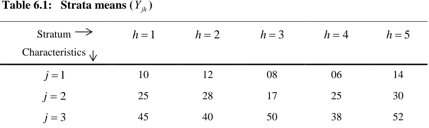
The data for three independent normal populations with the specification of strata means jh
Y
and the strata standard deviationsS
jh given in Tables 6.1 and 6.2 respectively are generated through the website “http://www.alewand.de/stattabneu/stattab.htm”.Table 6.1: Strata means (Y ) jh
Stratum
Characteristics
1
h h2 h3 h4 h5
1
j 10 12 08 06 14
2
j 25 28 17 25 30
3
Table 6.2: Stratum standard deviations (Sjh) for three characteristics and five strata
Stratum
Characteristics
1
h h2 h3 h4 h5
1
j 25 10 10 35 10
2
j 22 05 15 07 05
3
j 15 15 25 40 25
It should be noted that S12= S13= S15 = 10, S22= S25= 5, S31= S32= 15 and S33 = S35 = 25.
In the above situation, we have, for the first characteristic ( j 1), lj = 1 and there is only one group G11 with
11
g = 3, M11 = {2, 3, 5} and L1 = 3.
For the second characteristic (
j
2
),l
j= 1 and there is only one groupG
21 with 21g = 2, M21 = {2, 5} and L2 = 4.
For the third characteristic ( j 3), lj= 2 and there are two groups G31 and G32. For G31:g31 = 2, M31 = {1, 2},
and for G32: g32 = 2, M32 = {3, 5} and L3 = 3.
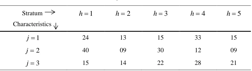
The preliminary samples sizes njh used to estimate Sjh are given in Table 6.3.
Table 6.3: Preliminary sample sizes (njh)
Stratum
Characteristics
1
h h2 h3 h4 h5
1
j 24 13 15 33 15
2
j 40 09 30 12 09
3
Table 6.4: Sample standard deviations (sjh)
Stratum
Characteristics
1
h h2 h3 h4 h5
1
j 21.1413 8.6060 9.6656 30.1319 8.8185
2
j 22.3244 4.6048 16.9006 5.7777 4.4331
3
j 15.0988 10.0282 23.2814 37.4376 24.8519
The sample data are generated through a computer program using the model
jh hi jh
jhi S Z Y
y ; j1,2, ,p; h1,2, ,L; i1,2,,Nh, where yjhi denote the value of the th
i observation in th
h stratum for the jth characteristic and Zhi are the values of the randomly selected standard normal variate Z.
Table 6.4 gives the estimated strata standard deviations sjh.
For the sake of comparisons the Averaged Neyman allocation for n = 100 using true standard deviations Sjh are worked out and are given in Table 6.5.
Table 6.5: Averaged Neyman allocation for n = 100 (Using Sjh)
With the help of available data the sampling variances of the estimates of the population means of the three characteristics (fpc ignored) under Averaged Neyman allocation given in Table 6.5 are obtained as
) (y1st
V = 3.348921164, V(y2st)= 1.413934847 and V(y3st)= 6.488945238 respectively.
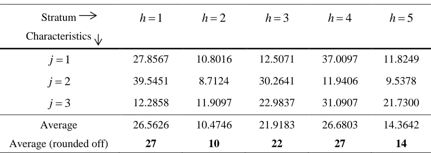
Using the sample standard deviations the Averaged Modified Neyman allocation for n = 100 are given in Table 6.6.
Stratum
Characteristics
1
h h2 h3 h4 h5
1
j 27.8567 10.8016 12.5071 37.0097 11.8249
2
j 39.5451 8.7124 30.2641 11.9406 9.5378
3
j 12.2858 11.9097 22.9837 31.0907 21.7300
Average 26.5626 10.4746 21.9183 26.6803 14.3642
Table 6.6: Averaged Modified Neyman allocation for n =100 (Using sjh)
Also the sampling variances of the estimates of the population means of the three characteristics (fpc ignored) under the Averaged Modified Neyman allocation given in Table 6.6 are obtained as
3 2.56984062 )
(y1st
V , V(y2st)1.475324005 and V(y3st)5.594390484 respectively.
Assuming that the true strata standard deviations Sjh are unknown but the information about the equality of some of the stratum standard deviations for a particular characteristic are available as stated after Table 6.2.
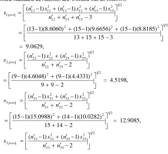
The pooled standard deviations are worked out as follows. 2 1 15 13 12 2 15 15 2 13 13 2 12 12 1 3 ) 1 ( ) 1 ( ) 1 ( 1 n n n s n s n s n s pool 2 1 2 2 2 3 15 15 13 ) 8185 . 8 )( 1 15 ( ) 6656 . 9 )( 1 15 ( ) 6060 . 8 )( 1 13 (
= 9.0629,
2 1 25 22 2 25 25 2 22 22 2 2 ) 1 ( ) 1 ( 1 n n s n s n s pool 2 1 2 2 2 9 9 ) 4331 . 4 )( 1 9 ( ) 6048 . 4 )( 1 9 (
= 4.5198,
2 1 32 31 2 32 32 2 31 31 3 2 ) 1 ( ) 1 ( 1 n n s n s n s pool 2 1 2 2 2 14 15 ) 0282 . 10 )( 1 14 ( ) 0988 . 15 )( 1 15 (
= 12.9085,
2 1 35 33 2 35 35 2 33 33 3 2 ) 1 ( ) 1 ( 2 n n s n s n s pool Stratum Characteristics 1
h h2 h3 h4 h5
1
j 27.0052 10.6565 13.8584 36.5258 11.9541
2
j 39.9037 7.9789 33.9080 9.8004 8.4091
3
j 13.3792 8.6140 23.1559 31.4812 23.3697
Average 26.7627 9.0831 23.6407 25.9358 14.5776
2 1 2 2
2 21 22
) 8519 . 24 )( 1 21 ( ) 2814 . 23 )( 1 22 (
= 24.0603,
where
k
pool j
s are as defined in (4.2).
For the first characteristic ( j1), the Modified Neyman allocation with pooled standard deviations will be the solution of the following NLPP
11
2 2
1
2 2
) 0629 . 9 ( ) 618 . 0 ( ) 1413 . 21 ( ) 196 . 0 ( Minimize
m
n
4
2 2
) 1319 . 30 ( ) 186 . 0 (
n
100 to
subject n1 m11 n4
and 2n1 98 (6.1)
309 6 m11
93 2n4 .
The values of n1, m11 and n4 according to the Modified Neyman allocation by using (1.2) for three strata are
1
n = 26.9963 27, m11 = 36.4899 36 and n4 36.5138 37.
These allocations already satisfy the limits of the sample sizes, thus they will solve the NLPP (6.1).
The values of n2, n3 and n5 are then reallocated out of m11 to their constituent strata using proportional allocation. This gives
11.0680 2
n 11, n3 12.8155 13 and n5 12.1165
12.Thus the optimum allocation with pooled strata variances for the first characteristic is *
11
n = 27, n12* = 11, * 13
n = 13, n14* = 37 and * 15
n = 12 with *
1
f = 2.356132272
Similarly, for second and third characteristics ( j2 and 3) the optimum allocations with pooled strata variances and the corresponding values of fj* are
2
j : n21* = 40, n22* = 8, n23* = 34, n*24 = 10 and n*25 = 8 with *
2
f = 1.202697797 3
j : *
31
n = 12, * 32
n = 11, * 33
n = 24, * 34
n = 31 and * 35
n = 22 with *
3
Now the pay-off matrix of the above formulated problems is given as: 56132272
. 2 ) ( 1* 1 nh
f f2(n1*h)1.944178835 f3(n1*h)6.209619712 458094757
. 4 ) ( 2* 1 n h
f f2(n*2h)1.202697797 f3(n*2h)9.633288575 028499035
. 3 ) ( *3 1 nh
f f2(n3*h)2.316987515 ( ) 4.931664512 *
3 3 n h
f
The upper and lower bound of each objective functions can be expressed as: 458094757
. 4 1
u
f 2.356132272
1 l
f 2.316987515
2 u
f 1.202697797
2 l f 633288575 . 9 3 u
f 4.931664512
1 l f
Let 1(njh),2(njh)and3(njh)be the fuzzy membership function of the objective function fj(njh),j1,2,3and they are defined as:
458094757 . 4 ) ( , 0 458094757 . 4 ) ( 356132272 . 2 , 101962485 . 2 ) ( 458094757 . 4 356132272 . 2 ) ( , 1 ) ( 1 1 1 1 1 1 1 1 1 1 h h h h h n f if n f if n f n f if n 316987515 . 2 ) ( , 0 316987515 . 2 ) ( 202697797 . 1 , 11428972 . 1 ) ( 316987515 . 2 202697797 . 1 ) ( , 1 ) ( 2 2 2 2 2 2 2 2 2 2 h h h h h n f if n f if n f n f if n 633288575 . 9 ) ( , 0 633288575 . 9 ) ( 931664512 . 4 , 70162406 . 4 ) ( 633288575 . 9 931664512 . 4 ) ( , 1 ) ( 3 3 3 3 3 3 3 3 3 3 h h h h h n f if n f if n f n f if n
On applying the max-addition operator, the MOSSD problem reduces to the problem as: Maximize 70162406 . 4 ) ( 11428972 . 1 ) ( 101962485 . 2 ) ( 09371222 .
6 f1 n1h f2 n2h f3 n3h
subject to n1 n2 n3 n4 n5 100 (6.2) and 2nh Nh,h1,2,,5.
In order to maximize the above problem, we have to minimize
70162406 . 4 ) ( 11428972 . 1 ) ( 101962485 . 2 )
( 1 2 2 3 3
1 nh f n h f n h
f
Minimize 5 2 2 5 2 2 5 2 2 4 2 2 4 2 2 4 2 2 3 2 2 3 2 2 3 2 2 2 2 2 2 2 2 2 2 2 1 2 2 1 2 2 1 2 2 70162406 . 4 ) 8519 . 24 ( ) 208 . 0 ( 11428972 . 1 ) 4331 . 4 ( ) 208 . 0 ( 101962485 . 2 ) 8185 . 8 ( ) 208 . 0 ( 70162406 . 4 ) 4376 . 37 ( ) 186 . 0 ( 11428972 . 1 ) 7777 . 5 ( ) 186 . 0 ( 101962485 . 2 ) 1319 . 30 ( ) 186 . 0 ( 70162406 . 4 ) 2814 . 23 ( ) 220 . 0 ( 11428972 . 1 ) 9006 . 16 ( ) 220 . 0 ( 101962485 . 2 ) 6656 . 9 ( ) 220 . 0 ( 70162406 . 4 ) 0282 . 10 ( ) 190 . 0 ( 11428972 . 1 ) 6048 . 4 ( ) 190 . 0 ( 101962485 . 2 ) 6060 . 8 ( ) 190 . 0 ( 70162406 . 4 ) 0988 . 15 ( ) 196 . 0 ( 11428972 . 1 ) 3244 . 22 ( ) 196 . 0 ( 101962485 . 2 ) 1413 . 21 ( ) 196 . 0 ( n n n n n n n n n n n n n n n
subject to n1 n2 n3 n4 n5 100 (6.3) and 2 nh Nh,h1,2,,5.
Thus we get Minimize 3 2 1 13751097 . 20 73110869 . 2 21337752 . 27 n n n
Z
5 4 046929969 . 8 29319393 . 26 n n
subject to n1 n2 n3 n4 n5 100 and 2nh Nh,h1,2,,5.
Using LINGO software package the solution to MOSSD problem is obtained as 1
n = 26.99968, n2 = 8.553362, n3 = 23.22578, n4 = 26.53927, n5=14.68191
Rounding off nh; h1,2,,5 to nearest integer values we get the compromise allocation as
1
n = 27, n2 = 9, n3 = 23, n4 = 27 and n5 = 15
with variances V(yjst); j1,2and3 under compromise allocation ignoring fpc as 2.51726615
,
1comp
V , 1.49467451
,
2 comp
V and 5.14560245
,
3 comp V
where, Vj,comp = V(yjst), j1,2and3 under compromise allocation ignoring fpc.
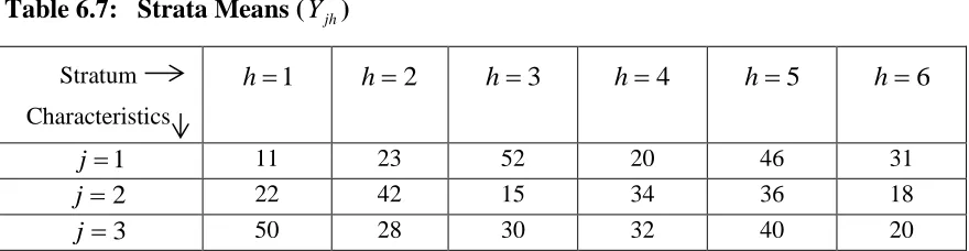
Table 6.7: Strata Means (Y ) jh
Stratum
Characteristics
1
h h2 h3 h4 h5 h6
1
j 11 23 52 20 46 31
2
j 22 42 15 34 36 18
3
j 50 28 30 32 40 20
Table 6.8: Stratum standard deviations (Sjh) for three characteristics and six strata
Stratum
Characteristics
1
h h2 h3 h4 h5 h6
1
j 35 10 9.5 15 9.8 21
2
j 19 20 30.3 30 17 24
3
j 32 25 12 40 24 18
It is assumed that the population of size N = 600 is divided into six strata with stratum sizes Nhand stratum weights Whas:
1
N = 93, N2= 99, N3= 105, N4= 96, N5= 132, N6= 75 and W1 = 0.155, W2= 0.165, W3= 0.175, W4= 0.160, W5= 0.220 and W6= 0.125 respectively.
Table 6.8 shows that for j1, S12, S13 and S15 are approximately equal, for j2 22
21 S
S and S23 S24 and for j3 S32 S35. Thus:
For j1, lj = 1, there is only one group G11with g11 = 3, M11 = { 2, 3, 5} and
1 L = 4.
For j2, lj2, there are two groups G21 and G22 with g21 = 2, M21 = { 1, 2} and g22 = 2, M22 = { 3, 4} respectively and L2 = 4.
For j3, l3 = 1, there is only one group G31 with g31 = 2, M31 = {2, 5} and 3
L = 5.
The preliminary samples sizes njh used to estimate Sjhare given in Table 6.9.
Table 6.9: Preliminary Sample Sizes (njh)
Stratum
Characteristics
1
h h2 h3 h4 h5 h6
1
j 13 15 13 37 16 26
2
j 18 23 21 16 27 15
3
The sample data are generated through a computer program using the same model as Example 1 that is,
jh hi jh
jhi S Z Y
y ; j1,2,...,p, h1,2,...,L and i1,2,...,Nh whereyjhi denote the value of the ithobservation in h th stratum for the th
j characteristic and Zhi are the values of the randomly selected standard normal variate Z.
The sample values of stratum standard deviations are summarized in Table 6.10.
Table 6.10: Sample standard deviations (sjh)
Stratum
Characteristics
1
h h2 h3 h4 h5 h6
1
j 15.9673 9.6105 10.2146 13.0483 11.3167 19.6771
2
j 20.9850 20.3869 31.8779 31.8431 13.9237 16.6347
3
j 38.1405 27.5064 10.7248 31.4545 24.7588 22.6623
Using the sample standard deviations the Averaged Modified Neyman allocation for n = 120 are given in Table 6.11.
Table 6.11: Averaged Modified Neyman allocation for n = 120 (Using sjh)
From the available data the sampling variances of the estimates of the population means of the three characteristics (fpc ignored) under the Averaged Modified Neyman allocation are obtained as
) ( 1 yst
V = 1.432900652, V2(yst) = 4.642929222 and V3(yst) = 5.810951230 respectively.
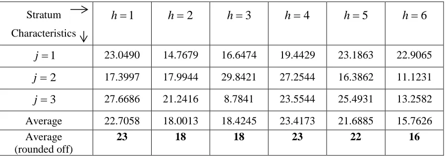
For the sake of comparisons the Averaged Neyman allocation for n = 120 using true standard deviations Sjh are given in Table 6.12.
Stratum
Characteristics
1
h h2 h3 h4 h5 h6
1
j 23.0490 14.7679 16.6474 19.4429 23.1863 22.9065
2
j 17.3997 17.9944 29.8421 27.2544 16.3862 11.1231
3
j 27.6686 21.2416 8.7841 23.5544 25.4931 13.2582
Average 22.7058 18.0013 18.4245 23.4173 21.6885 15.7626
Average (rounded off)
Table 6.12: Averaged Neyman allocation for n = 120 (Using Sjh)
With the help of available data the sampling variances of the estimates of the population means of the three characteristics (fpc ignored) under Averaged Neyman allocation are obtained as
) ( 1 yst
V = 2.344953919, V2(yst) = 4.876740281 and V3(yst) = 5.603878698 respectively.
Assuming that the true strata standard deviations Sjh are unknown but the information
about the equality of some of the standard deviations for a particular characteristic are available as stated after Table 6.8, pooled standard deviations are worked out using (4.2) as
1
1pool
s = 10.4370, 1
2pool
s = 20.6497, 2
2pool
s = 31.8630, 1
3pool
s = 26.3890.
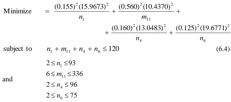
For the characteristic j1, the Modified Neyman allocation with pooled standard deviations will be the solution of the following NLPP:
11
2 2
1
2 2
) 4370 . 10 ( ) 560 . 0 ( ) 9673 . 15 ( ) 155 . 0 ( Minimize
m n
6
2 2
4
2 2
) 6771 . 19 ( ) 125 . 0 ( ) 0483 . 13 ( ) 160 . 0 (
n
n
120 to
subject n1 m11 n4 n6 (6.4)
and
75 2
96 2
336 6
93 2
6 4 11 1
n n m n
By using the formula (1.2) the modified Neyman allocation for four strata, are of n1, m11, 4
n and n6 given as:
1
n = 23.0817 23 m11 = 54.5089 55 n4 = 19.4705 19 n6 = 22.9390 23
Stratum
Characteristics
1
h h2 h3 h4 h5 h6
1
j 40.8958 12.4384 12.5326 18.0922 16.2528 19.7883
2
j 15.3070 17.1521 27.5604 24.9486 19.4391 15.5929
3
j 23.6990 19.7093 10.0338 30.5793 25.2280 10.7505
Average 26.6339 16.4333 16.7089 24.5400 20.3066 15.3772
Average (rounded off)
These allocations already satisfy the limits of sample sizes, thus they will solve the NLPP (6.4).
The sample size m11 to the combined stratum is reallocated to its constituent strata (2nd, 3rd and 5th) proportionally as:
2
n = 16.2054 16 n3 = 17.1875 17 and n5 = 21.6071 22
Thus the optimum values of the sample sizes to different strata for the first characteristic are:
* 11
n = 23, n12* = 16, n13* = 17, n14* = 19, n15* = 22 and n16* = 23 with *
1
f = 1.385622811
Similarly for the second and third characteristics ( j2and3), the individual optimum values of njh; j2,3, h1,2,...,6 are worked out as:
: 2
j n21* = 17, n*22= 18, n*23 = 30, n*24 = 27, n*25 = 17 and n26* = 11 with *
2
f = 4.194774309 :
3
j n31* = 27, n*32= 20, n33* = 9, n34* = 24, n*35 = 27 and n*36 = 13 with *
3
f = 5.487212235
Now the pay-off matrix of the above problems is given below: 385622811
. 1 ) ( 1* 1 nh
f f2(n1*h)4.978569804 f3(n1*h)6.044702086 389501246
. 2 ) ( 2* 1 n h
f f2(n*2h)4.194774309 ( ) 6.730451175 *
2 3 n h
f
584181422 .
1 ) ( 3* 1 n h
f f2(n3*h)6.172221739 f3(n3*h)5.487212235
The upper and lower bound of each objective functions can be expressed as: 389501246
. 2 1
u
f 1.385622811
1
l
f 6.172221739
2
u
f 4.194774309
2
l f
730451175 .
6 3
u
f 5.487212235
1
l f
Let 1(njh),2(njh)and3(njh)be the fuzzy membership function of the objective function fj(njh),j1,2,3and they are defined as:
389501246 .
2 ) ( , 0
389501246 .
2 ) ( 385622811 .
1 , 00387844
. 1
) ( 389501246 .
2
385622811 .
1 ) ( , 1
) (
1 1
1 1 1
1
1 1
1 1
h
h h
h
h
n f if
n f if
n f
n f if n
172221739 . 6 ) ( , 0 172221739 . 6 ) ( 194774309 . 4 , 97744743 . 1 ) ( 172221739 . 6 194774309 . 4 ) ( , 1 ) ( 2 2 2 2 2 2 2 2 2 2 h h h h h n f if n f if n f n f if n 730451175 . 6 ) ( , 0 730451175 . 6 ) ( 487212235 . 5 , 24323894 . 1 ) ( 730451175 . 6 487212235 . 5 ) ( , 1 ) ( 3 3 3 3 3 3 3 3 3 3 h h h h h n f if n f if n f n f if n
On applying the max-addition operator, the MOSSD problem reduces to the problem as: Maximize 24323894 . 1 ) ( 97744743 . 1 ) ( 00387844 . 1 ) ( 91521965 .
10 f1 n1h f2 n2h f3 n3h
subject to n1 n2 n3 n4 n5n6 120 (6.5) and 2 nh Nh,h1,2,,6.
In order to maximize the above problem, we have to minimize
24323894 . 1 ) ( 97744743 . 1 ) ( 00387844 . 1 )
( 1 2 2 3 3
1 nh f n h f n h
f
subject to the constraints as described below:
Minimize 6 2 2 6 2 2 6 2 2 5 2 2 5 2 2 5 2 2 4 2 2 4 2 2 4 2 2 3 2 2 3 2 2 3 2 2 2 2 2 2 2 2 2 2 2 1 2 2 1 2 2 1 2 2 24323894 . 1 ) 6623 . 22 ( ) 125 . 0 ( 97744743 . 1 ) 6347 . 16 ( ) 125 . 0 ( 00387844 . 1 ) 6771 . 19 ( ) 125 . 0 ( 24323894 . 1 ) 7588 . 24 ( ) 220 . 0 ( 97744743 . 1 ) 9237 . 13 ( ) 220 . 0 ( 00387844 . 1 ) 3167 . 11 ( ) 220 . 0 ( 24323894 . 1 ) 4545 . 31 ( ) 160 . 0 ( 97744743 . 1 ) 8431 . 31 ( ) 160 . 0 ( 00387844 . 1 ) 0483 . 13 ( ) 160 . 0 ( 24323894 . 1 ) 7248 . 10 ( ) 175 . 0 ( 97744743 . 1 ) 8779 . 31 ( ) 175 . 0 ( 00387844 . 1 ) 2146 . 10 ( ) 175 . 0 ( 24323894 . 1 ) 5064 . 27 ( ) 165 . 0 ( 97744743 . 1 ) 3869 . 20 ( ) 165 . 0 ( 00387844 . 1 ) 6105 . 9 ( ) 165 . 0 ( 24323894 . 1 ) 1405 . 38 ( ) 155 . 0 ( 97744743 . 1 ) 9850 . 20 ( ) 155 . 0 ( 00387844 . 1 ) 9673 . 15 ( ) 155 . 0 ( n n n n n n n n n n n n n n n n n n
On simplifying we get Minimize
3 2
1
75439250 .
21 79547140 .
24 56324029 .
39
n n
n
Z
6 5
4
66758129 .
14 78404490 .
34 84158531 .
37
n n
n
subject to n1 n2 n3 n4 n5n6 120, and 2 nh Nh,h1,2,,6.
Using LINGO software package the solution to MOSSD problem is obtained as 1
n = 23.72606, n2 = 18.78304, n3 = 17.59354, n4 = 23.20408, n5=22.24691, n6 =14.44638
Rounding off nh; h1,2, ,5 to nearest integer values we get the compromise allocation as
1
n = 24, n2 = 19, n3 = 18, n4 = 23, n5 = 22 and n6=14
with variances
V
(
y
jst)
;j
1
,
2
and
3
under compromise allocation ignoring fpc as 1.46846786, 1comp
V , V2,comp 4.52928072 and V3,comp 5.75905709 where, Vj,comp = V(yjst), j1,2and3 under compromise allocation ignoring fpc.
7. Conclusion
To validate the proposed compromise allocation, it is compared with some other existing compromise allocations and proportional allocation as well. Tables 7.1 and 7.2, for Examples 1 and 2 respectively, explore the performance of the proposed allocation and other comparative allocations.
The proportional allocation is worked out by
L h
nW
nh h: 1,2,..., , (7.1)
and its variance (ignoring fpc) is computed directly using the formula .
3 , 2 , 1 ; )
(
1 2 2
,
,
j n
s W y
V V
L
h h jh h prop
st j prop
j
The following averaged compromise allocations are selected for comparison. (i) Averaged Neyman allocation,
(ii) Averaged Modified Neyman allocation,
(iii) Averaged Allocation with Pooled Standard Deviations.
Kozak (2006b) considered five methods for working out the compromise allocation in multivariate stratified surveys. In the fifth method, Kozak minimized the sum of relative increases in the variances due to not using the individual optimum allocations. Thus the problem of allocation may be stated as the following NLPP
Minimize f(n1,n2,...,nL) =
p
j j j
V V
1 * subject to n n
L
h h
1
(7.2) and nh 0; h1,2,...,L.
Since the true Sjh are assumed to be unknown the objective function may be expressed as
p
j j j
V V
1 * ˆ ˆ
, where Vˆ and j
* ˆ
j
V are sample estimates of Vj and Vj*.
The solution to the NLPP (7.2), with objective as “Minimize
p
j j j
V V
1 * ˆ
ˆ
” is obtained by using Lagrange multiplier technique after ignoring non-negativity restrictions, is given as
L
h h h
h h h
b W
b W n n
1
; h1,2,...,L, (7.3)
where
p
j
j jh
h s V
b
1
* 2 ˆ and
2
1
* 1
ˆ
L
h
jh h
j W s
n
V . (7.4)
The allocations given by (7.3) are termed as “Kozak’s allocation” are placed for comparison in Tables 7.1 and 7.2.
The basis of comparison is the ‘TRACE’ (the sum of principal diagonal elements =
p
j
st j y
V 1
)
( ) of the variance-covariance matrix of the estimator of the jth population means Yj;j1,2,3. Since all the characteristics are assumed to be independent, the co-variances are zero. The relative efficiency (R. E.) of a compromise allocation with respect to the proportional allocation is defined as
comp prop T
T E
R. . / (Sukhatme et al. (1984)),
where Tprop represents the trace under proportional allocation and Tcomp represents the
trace under a compromise allocation.
The last columns of Tables 7.1 and 7.2 explain relative efficiency of all allocations, as discussed, with respect to proportional allocation.
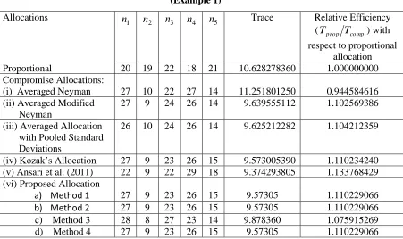
Table 7.1: Relative efficiencies of different compromise allocations as compared to the proportional allocation.
(Example 1) Allocations
1
n n2 n3 n4 n5 Trace Relative Efficiency
(Tprop Tcomp) with respect to proportional
allocation
Proportional 20 19 22 18 21 10.628278360 1.000000000
Compromise Allocations:
(i) Averaged Neyman 27 10 22 27 14
11.251801250 0.944584616 (ii) Averaged Modified
Neyman
27 9 24 26 14 9.639555112 1.102569386
(iii) Averaged Allocation with Pooled Standard Deviations
26 10 24 26 14 9.625212282 1.104212359
(iv) Kozak’s Allocation 27 9 23 26 15 9.573005390 1.110234240
(v) Ansari et al. (2011) 22 9 22 29 18 9.374293805 1.133768429 (vi) Proposed Allocation
a) Method 1 27 9 23 26 15 9.57305 1.110229066
b) Method 2 27 9 23 26 15 9.57305 1.110229066
c) Method 3 28 8 27 23 14 9.878360 1.075915269
d) Method 4 27 9 23 26 15 9.57305 1.110229066
Table 7.2: Relative efficiencies of different compromise allocations as compared to the proportional allocation.
(Example 2)
Allocations
1
n n2 n3 n4 n5 n6 Trace Relative Efficiency
(Tprop Tcomp) with respect to proportional
allocation
Proportional 19 20 21 19 26 15 12.137564700 1.000000000
Compromise Allocations:
(i) Averaged Neyman 27 16 17 25 20 15 12.825572900 0.946356533 (ii) Averaged Modified
Neyman
23 18 18 23 22 16 11.886781100 1.021097688
(iii) Averaged Allocation with Pooled Standard Deviations
22 18 19 23 22 16
11.878224270
1.021833266
(iv) Kozak’s Allocation 22 18 20 23 21 16 11.856593500 1.021973573
(v) Ansari et al. (2011) 23 19 19 24 21 14
11.836881600
1.025402222
(vi) Proposed Allocation
a) Method 1 24 19 18 23 22 14 11.85681 1.023678772
b) Method 2 24 19 18 23 22 14 11.85681 1.023678772
c) Method 3 24 19 18 24 23 12 11.88560 1.021199157
Acknowledgments
The authors are grateful to the Chief Editor and the learned Referees for their valuable comments. The first author is also grateful to the UGC Start up grant to carry out the research.
References
1. Ahsan, M. J. and Khan, S. U. (1977). Optimum allocation in multivariate stratified random sampling using prior information, Journal of Indian Statistical Association, 15, 57-67.
2. Ahsan, M. J. and Khan, S. U. (1982). Optimum allocation in multivariate stratified random sampling with overhead cost, Metrika, 29, 71-78.
3. Ahsan, M. J., Najmussehar and Khan, M. G. M. (2005). Mixed allocation in stratified sampling, Aligarh Journal of Statistics, 25, 87-97.
4. Ansari, A. H., Najmussehar and Ahsan, M. J. (2009). On multiple response stratified random sampling design, International Journal of Statistical Sciences, Kolkata, India, 1 (1), 1-11.
5. Ansari, A. H., Varshney, R., Najmussehar and Ahsan, M. J. (2011). An optimum multivariate-multiobjective stratified sampling design, Metron, Vol. LXIX (3), 227 – 250.
6. Aoyama, H. (1963). Stratified random sampling with optimum allocation for multivariate populations, Annals of the Institute of Statistical Mathematics, 14, 251 -258.
7. Arvanitis, L. G. and Afonja, B. (1971). Use of the generalized variance and the gradient projection method in multivariate stratified random sampling, Biometrics, 27, 119-127.
8. Bankier, M. D. (1988). Power allocations: Determining sample sizes for sub national areas, The American Statistician,42,174-177.
9. Bethel, J. (1989). Sample allocation in multivariate surveys, Survey Methodology, 15 (1), 47-57.
10. Chatterjee, S. (1967) A note on optimum allocation, Scandinavian Actuarial Journal,50,40-44.
11. Chatterjee, S. (1968). Multivariate stratified surveys, Journal of American Statistical Association, 63, 530-534.
12. Cochran, W. G. (1977). Sampling Techniques, 3rd ed., John Wiley and Sons, New York.
13. Dalenius, T. (1957). Sampling in Sweden: Contributions to the Methods and Theories of Sample Survey Practice,Almqvist and Wiksell, Stockholm.
15. Díaz-García, J. A. and Cortez, L. U. (2008). Multi-objective optimisation for optimum allocation in multivariate stratified sampling, Survey Methodology, 34 (2), 215-222.
16. Fatima, U., Varshney, R., Najmussehar and Ahsan, M.J. (2014). On Compromise Mixed Allocation in Multivariate Stratified Sampling with Random Parameters, Journal of Mathematical Modelling and Algorithms in Operations Research, Vol. 13(4), 523 – 536.
17. Folks, J. L. and Antle, C. E. (1965). Optimum allocation of sampling units to the strata when there are R responses of interest, Journal of the American Statistical Association, 60, 225-233.
18. Ghosh, S. P. (1958). A note on stratified random sampling with multiple characters, Calcutta Statistical Association Bulletin,8, 81-89.
19. Jahan, N., Khan, M. G. M. and Ahsan, M. J. (1994). A generalized compromise allocation, Journal of the Indian Statistical Association, 32, 95-101.
20. Khan, M. G. M., Ahsan, M. J. and Jahan, N. (1997). Compromise allocation in multivariate stratified sampling: an integer solution, Naval Research Logistics, 44, 69-79.
21. Khan, M. G. M., Khan, E. A. and Ahsan, M. J. (2003). An optimal multivariate stratified sampling design using dynamic programming, Australian & New Zealand Journal of Statistics, 45 (1),107-113.
22. Kokan, A. R. and Khan, S. (1967). Optimum allocation in multivariate surveys: An analytical solution, Journal of the Royal Statistical Society, Series B, 29 (1), 115-125.
23. Kozak, M. (2006a). Multivariate sample allocation: application of random search method, Statistics in Transition, 7 (4), 889-900.
24. Kozak, M. (2006b). On sample allocation in multivariate surveys, Communications in statistics-Simulation and Computation, 35, 901-910.
25. Kreienbrock, L. (1993). Generalized measures of dispersion to solve the allocation problem in multivariate stratified random sampling, Communications in Statistics-Theory and Methods, 22(1), 219-239.
26. Lingo User’s Guide (2001). LINGO-User’s Guide, Published by LINDO SYSTEM INC., 1415, North Dayton Street, Chicago, Illinois, 60622, USA.
27. Mahalanobis, P. C. (1944). On large-scale sample surveys, Philosophical Transactions of the Royal Society, Series B, 231,329-451.
28. Melaku, A. and Sadasivan, G. (1987). L1-norm and other methods for sample allocation in multivariate stratified surveys, Computational Statistics & Data Analysis, 5 (4),415-423.
30. Park, H., NA, S. and Jeon, J. (2007). Compromise allocation in univariate stratified sampling, Communications in Statistics-Theory and Methods, 36, 265-271.
31. Stuart, A. (1954). A simple presentation of optimum sampling results, Journal of Royal Statistical Society, Series B, 16 (2),239-241.
32. Sukhatme, P. V., Sukhatme, B. V., Sukhatme, S. and Asok, C. (1984). Sampling Theory of Surveys with Applications, 3rd ed., Iowa State University Press, Ames, Iowa and Indian Society of Agricultural Statistics, New Delhi.
33. Tiwari, R.N., Dharman, S. and Rao, J.R. (1987). Fuzzy Goal Programming - An Additive Model, Fuzzy Sets and Systems, 24, 27-34.
34. Varshney, R., Khan, M.G.M., Fatima, U. and Ahsan, M.J. (2015). Integer Compromise Allocation in Multivariate Stratified Surveys, Annals of Operations Research, Vol. 226 (1), 659 – 668.
35. Varshney, R., Najmussehar and Ahsan, M. J. (2012). An optimum multivariate stratified double sampling design in presence of non-response, Optimization Letters, Vol. 6(5), 993-1008.