Extended Half-Logistic Distribution with Theory and Lifetime Data Application

and Lifetime Data Application

Emrah Altun

Department of Statistics, Hacettepe University, Turkey. [email protected]

Muhammad Nauman Khan

Department of Mathematics, Kohat University of Science & Technology, Kohat, Pakistan [email protected]

Morad Alizadeh

Department of Statistics, Persian Gulf university, Bushehr, Iran [email protected]

Gamze Ozel

Department of Statistics, Hacettepe University, Turkey [email protected]

Nadeem Shafique Butt

Department of Family and Community Medicine, King Abdulaziz University Kingdom of Saudi Arabia

[email protected]

Abstract

In this paper, we introduce a new three-parameter lifetime model called the extended half-logistic (EHL) distribution. We derive various of its structural properties including moments, quantile and generating functions, mixture representation for probability density function, and reliability curves. The maximum likelihood, ordinary and weighted least square methods are used to estimate the model parameters. Simulation results to assess the performance of the estimation methods are discussed. We conclude that the maximum likelihood is the most suitable method to estimate model parameters for the small sample size. While the weighted least square method is the best for the large sample size. Finally, we prove empirically the importance and flexibility of the new model in modeling a real lifetime dataset.

Keywords: Half-logistic distribution, Meijer’s 𝐺–functions, Weighted Least Square.

AMS Classification: 62E10

1. Introduction

The statistical analysis and modeling of lifetime data are essential in almost all applied sciences including, biomedical science, engineering, finance, and insurance, among others. Many continuous distributions for the modeling lifetime data has been introduced in statistical literature including exponential, Lindley, gamma, log normal, half logistic, and Weibull. The half-logistic (HL) distribution has been used quite extensively in reliability and lifetime data analysis. The cumulative distribution function (cdf) of the HL distributed random variable 𝑋, with scale parameter (𝛽) is given by

The HL distribution does not provide enough flexibility for analyzing different types of lifetime data. Hence, it will be useful to consider other alternatives to this distribution for modelling purposes. Hence, our purpose is to provide a generalization that may be useful to more complex situations. Once the proposed distribution is quite flexible in terms of probability density function (pdf) and hazard rate function (hrf), it may provide an interesting alternative to describe income distributions and can also be applied in actuarial science, finance, bioscience, telecommunications and modelling lifetime data, for example. We introduce extended half-logistic (EHL) distribution using the HL distribution as the baseline distribution. The cdf and the pdf of the EHL distribution are, respectively, given by

𝐹(𝑥) =1−e−𝛽𝑥−𝜆𝑥𝛾

1+e−𝛽𝑥−𝜆𝑥𝛾 , 𝑥 > 0 , (1)

𝑓(𝑥) =2(𝛽+𝛾𝜆𝑥𝛾−1)e−𝛽𝑥−𝜆𝑥𝛾

(1+e−𝛽𝑥−𝜆𝑥𝛾₎2 , (2)

where 𝛼, 𝛽 > 0 and 𝛾 ∈ (0, ∞)\{1}. A random variable 𝑋 with pdf (2) is denoted by

𝑋~ 𝐸𝐻𝐿 (𝛽, 𝜆, 𝛾). The EHL distribution is much more flexible than the HL distribution and allows for greater flexibility of the tails.

In reliability studies, the hrf is an important characteristic and fundamental to the design of safe systems in a wide variety of applications. The corresponding hrf of the EHL distribution is obtained as

ℎ(𝑥) =(𝛽+𝜆 𝛾 𝑥_{1+e−𝛽 𝑥−𝜆 𝑥𝛾}𝛾−1) . (3)

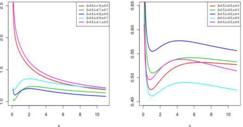
Figures 1 and 2 represents the pdf and hrf plots of the EHL distribution, respectively. As seen in Figure 1, the density function can take various forms depending on the parameter values. Figure 2 shows that the hrf of the EHL distribution has very flexible shapes, such as increasing, decreasing, upside-down bathtub. It is evident that the EHL distribution is much more flexible than the HL distribution. This attractive flexibility makes the hrf of the EHL useful and suitable for non-monotone empirical hazard behaviour which are more likely to be encountered or observed in real life situations.

Figure 2: Plots of the hrf of the EHL distribution for the selected parameter values.

For simulation from the EHL distribution, let U be a uniform variable on the unit interval (0, 1). Thus, by means of the inverse transformation method, we easily simulate data from the EHL by following equation:

𝛽 𝑥 + 𝜆 𝑥𝛾 _{+ log (}1−𝑈

1+𝑈) = 0. (4)

Theorem 1 provides a relation of the EHL distribution with HL distribution.

Theorem 1 Let 𝑋~EHL(𝛽, 𝜆, 𝛾, 𝑥).

If 𝑌 = 𝛽𝑥 + 𝜆𝑥𝛾, then 𝑌~𝐻𝐿 with 𝑠𝑐𝑎𝑙𝑒 = 1

The rest of the paper is outlined as follows. In Section 2, we discuss the distributional properties of the proposed distribution, including mixture representation for pdf, moments, moment generating function, and reliability curves. The asymptotic and shapes of the density and hazard rate functions are also investigated. In Section 3, maximum likelihood, ordinary and weighted least square methods are used to estimate model parameters. Section 4 presents a simulation study. Application with real lifetime data is considered in Section 5. Finally, Section 6 offers some concluding remarks.

2. Main properties

2.1 Asymptotic and Shapes

The asymptotics of equations (1), (2) and (3) as 𝑥 → 0 are given by

𝐹(𝑥)~1

𝑓(𝑥)~1

2 (𝛽 + 𝜆 𝛾 𝑥𝛾−1) as 𝑥 → 0, ℎ(𝑥)~1

2 (𝛽 + 𝜆 𝛾 𝑥𝛾−1) as 𝑥 → 0,

The asymptotics of equations (1), (2) and (3) as 𝑥 → ∞ are given by

1 − 𝐹(𝑥)~2 e−𝛽 𝑥−𝜆 𝑥𝛾 _{as 𝑥 → ∞,}

𝑓(𝑥)~2(𝛽 + 𝜆 𝛾 𝑥𝛾−1_{) e}−𝛽 𝑥−𝜆 𝑥𝛾

as 𝑥 → ∞, ℎ(𝑥)~2(𝛽 + 𝜆 𝛾 𝑥𝛾−1_{) as 𝑥 → ∞.}

2.2 Mixture for pdf

In this subsection, we provide alternative mixture representation for the pdf of the EHL distribution. Despite the fact that the pdf of the EHL require mathematical functions that are widely available in modern statistical packages, frequently analytical and numerical derivations take advantage of power series for the pdf. Some useful expansions for (2) can be derived by using the concept of power series. Using generalized binomial expansion, we obtain the pdf of the EHL as

𝑓(𝑥) = 2 ∑

∞

𝑚=0

(−2_𝑚 ) (𝛽 + 𝜆 𝛾 𝑥𝛾−1_{) e}−𝛽(𝑚+1) 𝑥−𝜆 (𝑚+1) 𝑥𝛾

= ∑∞_𝑚=0 𝑉_𝑚(𝛽 + 𝜆 𝛾 𝑥𝛾−1) e−𝛽(𝑚+1) 𝑥−𝜆 (𝑚+1) 𝑥𝛾, (5)

where 𝑉_𝑚 = 2 (−1)𝑚 (𝑚 + 1).

It is clear from (5) that 𝑓(𝑥) can be expressed as infinite linear combinations of the modified Weibull (MW) distributions and hence many properties of the EHL distribution can be deduced from the corresponding ones of the MW distribution. In what follows, we discuss some properties of the EHL distribution and consider several associated statistical functions.

2.3 Moments and moment generating function

We now obtain representations of the moments and moment generating function (mgf) of the EHL random variable on the basis of the following result developed in Saboor et al. (2012).

∫

∞

0

𝑥𝜂−1_e−𝜃 𝑥𝑘_e𝑠 𝑥_{𝑑𝑥 =}(2𝜋)1−(q+p)/2 q1/2p 𝜂−1/2

(−s)𝜂

× 𝐺_𝑝,𝑞𝑞,𝑝((−𝑝_𝑠)𝑝 (𝜃_𝑞)𝑞 |1 −

𝑖+𝜂 𝑝

𝑗/𝑞 ,

, 𝑖 = 0,1, . . . . , 𝑝 − 1

𝑗 = 0,1, . . . . , 𝑞 − 1), (6)

where ℜ(𝜂), ℜ(𝜃), ℜ(𝑠) < 0 and 𝑘 is a rational number such that 𝑘 = 𝑝/𝑞, where 𝑝 and

Using (6), the 𝑟𝑡ℎ order moment and mgf of the EHL distribution can be expressed in terms of Meijer’s 𝐺–functions as

𝐸(𝑋𝑟_{) = 𝛽 ∑} ∞

𝑚=0

𝑉_𝑚 (2𝜋)1−(𝑞+𝑝)/2𝑞1/2𝑝𝑟+1/2 (𝛽(𝑚 + 1))𝑟+1

× 𝐺_𝑝,𝑞𝑞,𝑝(( 𝑝 𝛽(𝑚 + 1))

𝑝

(𝜆(𝑚 + 1)

𝑞 )

𝑞

|1 −

𝑖 + 𝑟 + 1

𝑝 ,

𝑗/𝑞,

𝑖 = 0,1, … , 𝑝 − 1 𝑗 = 0,1, … , 𝑞 − 1)

+𝜆 𝛾 ∑

∞

𝑚=0

𝑉_𝑚 (2𝜋)1−(𝑞+𝑝)/2𝑞1/2𝑝𝑟+𝛾−1/2 (𝛽(𝑚 + 1))𝑟+𝛾

× 𝐺_𝑝,𝑞𝑞,𝑝((_𝛽(𝑚+1)𝑝 )𝑝(𝜆(𝑚+1)_𝑞 )𝑞|1 −

𝑖+𝑟+𝛾 𝑝 ,

𝑗/𝑞,

𝑖 = 0,1, … , 𝑝 − 1

𝑗 = 0,1, … , 𝑞 − 1), (7)

The ℎ𝑡ℎ order negative moment can readily be determined by replacing 𝑟 with −ℎ in (7). The mgf of the EHL distribution is given by

𝑀(𝑡) = 𝛽 ∑

∞

𝑚=0

𝑉_𝑚 (2𝜋)1−(𝑞+𝑝)/2 𝑞1/2𝑝 1/2 𝛽(𝑚 + 1) − 𝑡

× 𝐺_𝑝,𝑞𝑞,𝑝(( 𝑝

𝛽(𝑚 + 1) − 𝑡)

𝑝

(𝜆(𝑚 + 1)

𝑞 )

𝑞

|1 − 𝑖 + 1

𝑝 ,

𝑗/𝑞,

𝑖 = 0,1, … , 𝑝 − 1 𝑗 = 0,1, … , 𝑞 − 1)

+𝜆 𝛾 ∑

∞

𝑚=0

𝑉_𝑚 (2𝜋)1−(𝑞+𝑝)/2 𝑞1/2𝑝 𝛾−1/2 (𝛽(𝑚 + 1) − 𝑡)𝛾

× 𝐺_𝑝,𝑞𝑞,𝑝((_{𝛽(𝑚+1)−𝑡}𝑝 )𝑝(𝜆(𝑚+1)_𝑞 )𝑞|1 −

𝑖+𝛾 𝑝 ,

𝑗/𝑞,

𝑖 = 0,1, … , 𝑝 − 1

𝑗 = 0,1, … , 𝑞 − 1). (8)

The skewness and kurtosis measures can be obtained from the ordinary moment using well-known relationships. Figure 3 displays the mean, variance, skewness and kurtosis of the EHL distribution for 𝛽 = 2. Based on the plots given in Figure 3, we conclude: 1. if 𝜆 increases, mean decreases; if 𝛾 increases, mean increases

2. if 𝜆 increases, variance decreases; if 𝛾 increases, variance increases

3. 𝛾 parameter has more significant effect on skewness and kurtosis measures than 𝜆 parameter,

In the rest of this section, we use the following lemma:

Lemma 1 Let

𝐽(𝑥; 𝑟, 𝜃) = ∫

𝑥

0

𝑦 𝑟_{𝑓(𝑦) d𝑦 = ∑} ∞

𝑚,s=0

𝑉_𝑚(−1)𝑠

𝑠! {𝛽(𝑚 + 1)}𝑠

× ∫

𝑥

0

𝑦𝑠+𝑟 _{(𝛽 + 𝜆 𝛾 𝑦}𝛾−1_{) e}−𝜆(𝑚+1) 𝑦𝛾 _{d𝑦, 𝑟 = 1,2, … ,}

where 𝜃 = (𝛽, 𝜆, 𝛾). Then, we have

𝐽(𝑥; 𝑟, 𝜃) = ∑

∞

𝑚,s=0

𝑉_𝑚(−1)𝑠

𝑠! {𝛽(𝑚 + 1)}𝑠

× { 𝛽 𝑞 𝑥𝑝 (𝑗+𝑟+1) 𝑝 (2 𝜋)(𝑞−1)/2

× 𝐺_{𝑝,𝑝+𝑞}𝑞,𝑝 ((𝜆(𝑚+1))_𝑞𝑞 𝑞 𝑥𝑝|

−𝑗−𝑟 𝑝 , 1−𝑗−𝑟 𝑝 , … , 𝑝−𝑗−𝑟−1 𝑝 , −

0 ,−𝑗−𝑟−1_𝑝 ,𝑗+𝑟_𝑝 , … ,𝑝−𝑗−𝑟−2_𝑝 )

+𝜆 𝑥𝑝 (𝑗+𝑟+𝛾) (2𝜋)(𝑞−1)/2

× 𝐺_{𝑝,𝑝+𝑞}𝑞,𝑝 ((𝜆(𝑚+1))𝑞 𝑥𝑝

𝑞𝑞 | −𝑗−𝑟−𝛾+1 𝑝 , 2−𝑗−𝑟−𝛾 𝑝 , … , 𝑝−𝑗−𝑟−𝛾 𝑝 , −

0 ,−𝑗−𝑟−𝛾_𝑝 ,𝑗+𝑟+𝛾−1_𝑝 , … ,𝑝−𝑗−𝑟−𝛾−1_𝑝 )}.

Proof 1 The proof can be obtained by noting that the arbitrary function 𝑒−𝑔(𝑥) =

𝐺_0,11,0(𝑔(𝑥) |−_{0 )}, letting 𝑘 = 𝑝/𝑞 where 𝑝 ≥ 1 , 𝑞 ≥ 1 are natural co-prime numbers, and making use of the identity

∫𝑥

0

𝑦𝑡 _𝐺

0,11,0(𝜆(𝑚 + 1)𝑦 𝑝

𝑞_{|0) d𝑦}

= 𝑞 𝑥𝑝 (𝑡+1)

𝑝(2𝜋)(𝑞−1)/2 𝐺𝑝,𝑝+𝑞𝑞,𝑝 (

(𝜆(𝑚+1))𝑞 _𝑥𝑝

𝑞𝑞 | −𝑡 𝑝 , 1−𝑡 𝑝 , … , 𝑝−𝑡−1 𝑝 , −

0 ,−𝑡−1_𝑝 ,_𝑝𝑡 , … ,𝑝−𝑡−2_𝑝 ) ,

which results from Equation (13) of Cordeiro et al. (2014).

2.4 Conditional moments and mean deviations

In connection with lifetime distributions, it is important to determine the conditional moments 𝐸(𝑋𝑟|𝑋 > 𝑡),𝑟 = 1,2, ⋯, which are of interest in predictive inference. The 𝑟𝑡ℎ conditional moment of the EHL distribution can be obtained as

𝐸(𝑋𝑟_{|𝑋 > 𝑡) =} 1

𝑆(𝑡)[𝐸(𝑋𝑟) − ∫

𝑡

0

𝑥 𝑟_{𝑓(𝑥) d𝑥]}

=1+e_{2 e−𝛽 𝑥−𝜆 𝑥𝛾}−𝛽 𝑥−𝜆 𝑥𝛾{𝐸(𝑋𝑟_{) − 𝐽(𝑡; 𝑟, 𝜃)}. (9)}

mean and median. The mean deviations of 𝑋 about the mean 𝜇 = 𝐸(𝑋) and about the median 𝑀 can be expressed as 𝛿 = 2𝜇𝐹(𝜇) − 2𝑚(𝜇) and 𝜂 = 𝜇 − 2𝑚(𝑀), where 𝐹(𝜇) is calculated from (1) and

𝑚(𝑧) = ∫₀𝑧 𝑥 𝑓(𝑥)𝑑𝑥 = 𝐽(𝑧; 1, 𝜃). (10)

2.5 Reliability curves

The Bonferroni and Lorenz curves have various applications in economics, reliability, insurance and medicine. The Bonferroni curve 𝐵_𝐹[𝐹(𝑥)] for the EHL distribution is given as

𝐵_𝐹[𝐹(𝑥)] = 1

𝐸(𝑋). 𝐹(𝑥)∫

𝑥

0

𝑦𝑓(𝑦)d𝑦 = 𝐽(𝑥; 1, 𝜃) 𝐸(𝑋). 𝐹(𝑥).

Then, the Lorenz curve of 𝐹 is obtained as

𝐿_𝐹[𝐹(𝑥)] =𝐽(𝑥;1,𝜃)

𝐸(𝑋) . (11)

The scaled total time on test transform of a distribution function 𝐹 (Pundir et al. (2005)) is defined by 𝑆_𝐹[𝐹(𝑡)] =_𝐸(𝑋)1 ∫₀𝑡 𝐹̅(𝑦)𝑑𝑦, and it is important for the ageing properties of

the underlying distribution and can be applied to solve geometrically some stochastic maintenance problems.

3. Estimation and inference

In this section, we obtain the maximum likelihood (ML), least square (LS) and weighted least square (WLS) estimates of the parameters of the EHL distribution taken a random sample with inference on those parameters. Further, some goodness-of-fit statistics are given to compare the density estimates and selection of the models.

3.1 Maximum Likelihood Estimation

Using the log-likelihood of the sample in conjunction with the NMaximize command in the symbolic computational package Mathematica, we can estimate the unknown parameters of a distribution. Given the observed values 𝑥_𝑖, 𝑖 = 1, … , 𝑛 of the taken sample from the EHL distribution, then the maximum likelihood estimators (MLEs) of the parameters are obtained by maximization of the log-likelihood function given by

ℓ(𝑥_𝑖; 𝜃) = ℓ(𝑥_𝑖, 𝛽, 𝜆, 𝛾) = 𝑛log(2) + ∑𝑛

𝑖=1 log(𝛽 + 𝛾𝜆𝑥𝑖𝛾−1) − ∑𝑛𝑖=1 (𝛽𝑥𝑖+

𝜆𝑥𝑖𝛾) − 2 ∑𝑛𝑖=1 log(1 + e−𝛽𝑥𝑖−𝜆𝑥𝑖 𝛾

) , (12)

and the associated nonlinear log-likehood system ∂ℓ(𝜃)

∂𝜃 = 0, where

∂ℓ(𝜃)

∂𝛽 = − ∑

𝑛

𝑖=1

𝑥𝑖 − 2 ∑ 𝑛

𝑖=1

− e

−𝛽𝑥𝑖−𝜆𝑥𝑖𝛾𝑥_𝑖

1 + e−𝛽𝑥𝑖−𝜆𝑥_𝑖𝛾+ ∑ 𝑛

𝑖=1

1

𝛽 + 𝛾𝜆𝑥_𝑖−1+𝛾 = 0, ∂ℓ(𝜃)

∂𝜆 = − ∑

𝑛

𝑖=1

𝑥_𝑖𝛾 − 2 ∑

𝑛

𝑖=1

− e

−𝛽𝑥𝑖−𝜆𝑥𝑖𝛾𝑥 𝑖𝛾

1 + e−𝛽𝑥𝑖−𝜆𝑥𝑖𝛾

+ ∑

𝑛

𝑖=1

𝛾𝑥_𝑖−1+𝛾

𝛽 + 𝛾𝜆𝑥_𝑖−1+𝛾 = 0, ∂ℓ(𝜃)

∂𝛾 = − ∑

𝑛

𝑖=1

𝜆log[𝑥_𝑖]𝑥_𝑖𝛾− 2 ∑

𝑛

𝑖=1

−e−𝛽𝑥𝑖−𝜆𝑥𝑖

𝛾

𝜆log[𝑥𝑖]𝑥𝑖𝛾

+ ∑

𝑛

𝑖=1

𝜆𝑥_𝑖−1+𝛾+ 𝛾𝜆log[𝑥𝑖]𝑥𝑖−1+𝛾

𝛽 + 𝛾𝜆𝑥_𝑖−1+𝛾 = 0.

By solving equations above simultaneously, we obtain the MLEs of the parameters. The numerical iterative techniques may be used for estimating the parameters and the global maxima of the log-likelihood is possible to investigate by putting different starting values for the parameters. The information matrix will be required for interval estimation. The elements of the 3 × 3 total observed information matrix 𝐽(𝜃) = 𝐽𝑟𝑠(𝜃) for 𝑟, 𝑠 = 𝛽, 𝜆, 𝛾, can be obtained from authors upon request.

3.2 Ordinary and Weighted Least-Square Estimators:

Let 𝑥₁, 𝑥₂, 𝑥₃, ⋯,𝑥_𝑛 denotes the ordered sample of the random sample of size n from the EHL distribution function F(⋅). The least square estimators (LSEs) can be obtained by minimizing

𝐿(Θ) = ∑𝑛

𝑖=1 (1−e

−𝛽𝑥𝑖−𝜆𝑥𝑖𝛾 1+e−𝛽𝑥𝑖−𝜆𝑥𝑖𝛾−

𝑖 𝑛+1)

2

, (13)

with respect to the unknown parameters. The associated nonlinear equations ∂𝐿(Θ)

∂Θ = 0

are given by

∂𝐿(Θ) ∂𝛽 = ∑

𝑛

𝑖=1 2 (1−e

−𝛽𝑥𝑖−𝜆𝑥𝑖𝛾

1+e−𝛽𝑥𝑖−𝜆𝑥𝑖𝛾− 𝑖 1+𝑛) (

e−𝛽𝑥𝑖−𝜆𝑥𝑖𝛾(1−e−𝛽𝑥𝑖−𝜆𝑥𝑖𝛾)𝑥𝑖

(1+e−𝛽𝑥𝑖−𝜆𝑥𝑖𝛾)

2 + e

−𝛽𝑥𝑖−𝜆𝑥𝑖𝛾𝑥𝑖

1+e−𝛽𝑥𝑖−𝜆𝑥𝑖𝛾) = 0,

∂𝐿(Θ) ∂𝜆 = ∑

𝑛

𝑖=1 2 (1−e

−𝛽𝑥𝑖−𝜆𝑥𝑖𝛾

1+e−𝛽𝑥𝑖−𝜆𝑥𝑖𝛾− 𝑖 1+𝑛) (

e−𝛽𝑥𝑖−𝜆𝑥𝑖𝛾(1−e−𝛽𝑥𝑖−𝜆𝑥𝑖𝛾)𝑥_𝑖𝛾

(1+e−𝛽𝑥𝑖−𝜆𝑥𝑖𝛾)

2 +

e−𝛽𝑥𝑖−𝜆𝑥𝑖𝛾𝑥_𝑖𝛾

1+e−𝛽𝑥𝑖−𝜆𝑥𝑖𝛾) = 0,

∂𝐿(Θ)

∂𝛾 = ∑

𝑛

𝑖=1

2 (1 − e−𝛽𝑥𝑖−𝜆𝑥𝑖

𝛾

1 + e−𝛽𝑥𝑖−𝜆𝑥_𝑖𝛾−

𝑖 1 + 𝑛)

× (e

−𝛽𝑥𝑖−𝜆𝑥𝑖𝛾(1 − e−𝛽𝑥𝑖−𝜆𝑥𝑖𝛾) 𝜆log[𝑥_𝑖]𝑥_𝑖𝛾

(1 + e−𝛽𝑥𝑖−𝜆𝑥𝑖𝛾)

2 +

e−𝛽𝑥𝑖−𝜆𝑥𝑖𝛾𝜆log[𝑥_𝑖]𝑥_𝑖𝛾

1 + e−𝛽𝑥𝑖−𝜆𝑥_𝑖𝛾 ) = 0.

Solving this nonlinear equations system simultaneously, we obtain the LSEs of the parameters.

The weighted least square estimators (WLSEs) can be obtained by minimizing

𝐿(Θ) = ∑𝑛

𝑖=1 (𝑛+1) 2_(𝑛+2) 𝑖(𝑛−𝑖+1) (

1−e−𝛽𝑥𝑖−𝜆𝑥𝑖𝛾 1+e−𝛽𝑥𝑖−𝜆𝑥𝑖𝛾−

𝑖 𝑛+1)

2

, (14)

with respect to the unknown parameters. The associated nonlinear equations ∂𝐿(Θ)_∂Θ = 0 are given by

∂𝐿(Θ)

∂𝛽 = ∑

𝑛

𝑖=1

2(𝑛 + 1)2_{(𝑛 + 2)}

𝑖(𝑛 − 𝑖 + 1) (

1 − e−𝛽𝑥𝑖−𝜆𝑥𝑖𝛾

1 + e−𝛽𝑥𝑖−𝜆𝑥_𝑖𝛾−

× (e

−𝛽𝑥𝑖−𝜆𝑥𝑖𝛾(1 − e−𝛽𝑥𝑖−𝜆𝑥𝑖𝛾) 𝑥_𝑖

(1 + e−𝛽𝑥𝑖−𝜆𝑥𝑖𝛾)

2 +

e−𝛽𝑥𝑖−𝜆𝑥𝑖𝛾𝑥_𝑖

1 + e−𝛽𝑥𝑖−𝜆𝑥𝑖𝛾

) = 0,

∂𝐿(Θ)

∂𝜆 = ∑

𝑛

𝑖=1

2(𝑛 + 1)2_{(𝑛 + 2)}

𝑖(𝑛 − 𝑖 + 1) (

1 − e−𝛽𝑥𝑖−𝜆𝑥𝑖𝛾

1 + e−𝛽𝑥𝑖−𝜆𝑥_𝑖𝛾−

𝑖 1 + 𝑛)

× (e

−𝛽𝑥𝑖−𝜆𝑥𝑖𝛾(1 − e−𝛽𝑥𝑖−𝜆𝑥𝑖𝛾) 𝑥_𝑖𝛾

(1 + e−𝛽𝑥𝑖−𝜆𝑥_𝑖𝛾₎2

+ e−𝛽𝑥𝑖−𝜆𝑥𝑖

𝛾

𝑥_𝑖𝛾 1 + e−𝛽𝑥𝑖−𝜆𝑥𝑖𝛾

) = 0,

∂𝐿(Θ)

∂𝛾 = ∑

𝑛

𝑖=1

2(𝑛 + 1)2_{(𝑛 + 2)}

𝑖(𝑛 − 𝑖 + 1) (

1 − e−𝛽𝑥𝑖−𝜆𝑥𝑖𝛾

1 + e−𝛽𝑥𝑖−𝜆𝑥_𝑖𝛾−

𝑖 1 + 𝑛)

× (e

−𝛽𝑥𝑖−𝜆𝑥𝑖𝛾(1 − e−𝛽𝑥𝑖−𝜆𝑥𝑖𝛾) 𝜆log[𝑥_𝑖]𝑥_𝑖𝛾

(1 + e−𝛽𝑥𝑖−𝜆𝑥_𝑖𝛾₎2

+e−𝛽𝑥𝑖−𝜆𝑥𝑖

𝛾

𝜆log[𝑥_𝑖]𝑥_𝑖𝛾 1 + e−𝛽𝑥𝑖−𝜆𝑥𝑖𝛾

) = 0.

Then, the WLSEs of the parameters are obtained by solving this nonlinear equations system simultaneously.

To check the goodness-of-fit of some statistical models defined in Section 5, we use Kolmogorov-Smirnov (K-S) test with their p-values to compare the fitted models. These statistics are used to evaluate how closely a specific distribution with cdf(⋅) fits the corresponding empirical distribution for a given data set. The distribution with better fit than the others will be the one having the smallest statistics and largest 𝑝-value.

4. Simulation Study

In this section, we consider MLE, LSE and WLSE methods for estimating unknown parameters of EHL distribution. We compare the parameter estimation efficiency of MLE, LSE and WLSE methods for the parameters of EHL distribution by means of Monte Carlo simulation. The following simulation procedure is implemented:

1. Set the sample size 𝑛 and the vector of parameters 𝜽 = (𝛽, 𝜆, 𝛾),

2. Generate random observations from the 𝐸𝐻𝐿(𝛽, 𝜆, 𝛾) distribution with size 𝑛,

3. Using the generated random observations in Step 2, estimate 𝜽̂ by means of MLE and LSE methods,

4. Repeat the steps 2 and 3 𝑁 times,

5. Using 𝜽̂ and 𝜽 compute the mean relative estimates (MREs) and mean square errors (MSEs) with the following equations:

𝑀𝑅𝐸 = ∑𝑁 𝑗=1 𝜽̂𝑖,𝑗/𝜽𝐢 𝑁 , 𝑀𝑆𝐸 = ∑𝑁 𝑗=1

(𝜽̂𝐢,𝐣−𝜽𝐢)2

The simulation results are computed with software R. The chosen parameters of simulation study are 𝜽 = (𝜆 = 0.5, 𝛽 = 3, 𝛾 = 2), 𝑁 = 1.000 and 𝑛 =

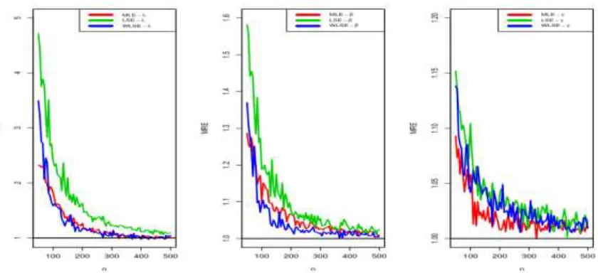
(50,55,60, . . . ,500). We expect that MREs are closer to one when the MSEs are near zero. Figures 3 and 4 represents estimated MSEs and MREs by means of the MLE and LSE methods, respectively. Based on Figures 3 and 4, the MSE of all estimates tend to zero for large 𝑛 and also as expected, the values MREs tend to one. It is clear that the estimates of parameters are asymptotically unbiased. The MLE and WLSE methods approach to nominal values of the MSEs and MREs faster than the LSE method. The MLE method exhibits better performance than the WLSE method for small sample size. Therefore, the MLE is more suitable method than others for estimating parameters of the EHL distribution for small sample size. While the WLSE method is the best to estimate EHL parameters for large sample size.

Figure 4: Estimated MSEs of the selected parameters for the MLE, LSE and WLSE methods.

5. Application

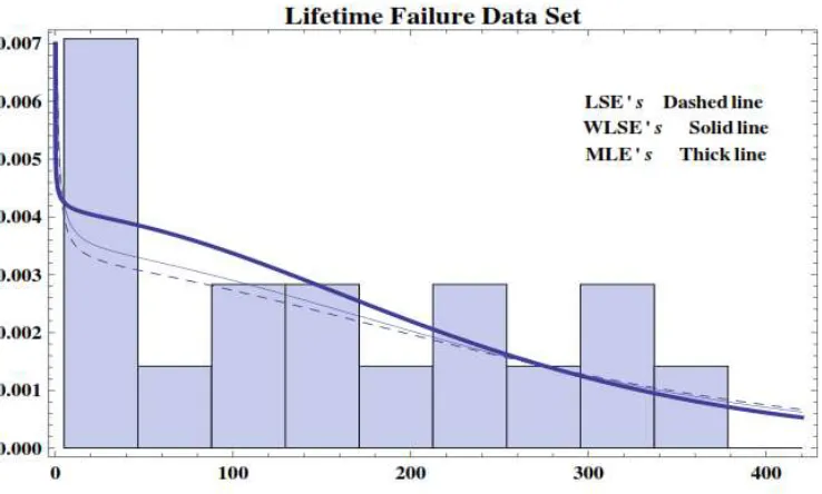
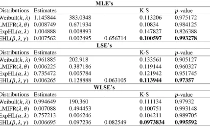
In this section, we analyze a real data set to demonstrate the performance of the EHL distribution in practice. The data used here are the lifetime failure data of an electronic device analyzed by Wang (2000). Using three different estimation methods given in Section 3, we fit the following distributions to the data: the Weibull distribution, a lifetime model with increasing failure rate (LMIFR) (Bakouch et al. 2014) and the exponentiated half-logistic (ExpHL) distribution (Gui (2015)). The MLEs, LSEs and WLSEs are listed in Table 1, respectively, with Kolmogorov-Smirnov (K-S) test and corresponding 𝑝-value for the fitted models. It is clear that the EHL model is the best among the fitted models since it corresponds to the smallest values of the statistics with larger 𝑝-value for all the three estimation methods. Further, it can be observed that the MLEs and WLSEs perform better than LSEs. This conclusion is again confirmed by a visual comparison of the histogram of the data for the fitted pdf of EHL distribution using the estimates given in Table 1 with three methods. The plots of the fitted EHL are shown in Figure 6 for the lifetime failure of an electronic device data. As seen from Figure 5, the EHL distribution appears to provide a closer fit to the histogram with the MLEs and WLSEs than the LSEs.

Table 1: Comparison of fit of EHL using different methods of estimation for device failure data

MLE’s

Distributions Estimates K-S 𝑝-value

Weibull(𝑘, 𝜆) 1.145844 383.0348 0.113206 0.975172

LMIFR(𝜆, 𝜃) 0.008749 0.671934 0.10834 0.984125

ExpHL(𝛼, 𝜆) 1.004888 0.008893 0.147827 0.826388

EHL(𝛽, 𝜆, 𝛾) 0.007562 0.002495 0.656714 0.100597 0.993278

LSE’s

Distributions Estimates K-S 𝑝-value

Weibull(𝑘, 𝜆) 0.961885 202.918 0.133561 0.905127

LMIFR(𝜆, 𝜃) 0.006225 0.387186 0.119144 0.960327

ExpHL(𝛼, 𝜆) 0.735472 0.005784 0.121942 0.951745

EHL(𝛽, 𝜆, 𝛾) 0.006265 0.128888 0.063105 0.113944 0.97357

WLSE’s

Distributions Estimates K-S 𝑝-value

Weibull(𝑘, 𝜆) 0.994649 190.360 0.111134 0.97932

LMIFR(𝜆, 𝜃) 0.007088 0.494453 0.100751 0.993148

ExpHL(𝛼, 𝜆) 0.757213 0.006246 0.104211 0.989705

EHL(𝛽, 𝜆, 𝛾) 0.006695 0.097236 0.082549 0.0973834 0.995592

6. Conclusion

A new three parameter lifetime distribution named, “extended half-logistic distribution” has been suggested for modeling lifetime data sets from engineering and medical science. Its important mathematical and statistical properties including shape, moments, hazard rate function, mixture representation of density function have been discussed. The maximum likelihood, ordinary and weighted least square methods ehave also been discussed for estimating its parameter. Finally, the goodness of fit test for the real lifetime dataset have been presented to demonstrate the applicability and comparability of Weibull, lifetime model with increasing failure rate, exponentiated half-logistic distributions and proposed extended half-logistic distribution for modeling lifetime datasets.

References

1. H. S. Bakouch, M. A. Jazi, S. Nadarajah, A. Dolati and R. Roozegar, A lifetime model with increasing failure rate, Applied Mathematical Modelling, 38 (2014) 5392–5406.

2. G.M. Cordeiro, E.M.M. Ortega, A.J. Lemonte, The exponential–Weibull lifetime distribution, Journal of Statistical Computation and Simulation, 84 (2014) 2592– 2606.

4. Saboor, S.B. Provost, M. Ahmad, The moment generating function of a bivariate gamma-type distribution, Applied Mathematics and Computation, 218(24) (2012) 11911–11921.

5. S. Pundir, S. Arora, K. Jain, Bonferroni curve and the related statistical inference, Statistics and Probability Letters, 75 (2005) 140-–150.