www.earth-surf-dynam.net/2/155/2014/ doi:10.5194/esurf-2-155-2014
©Author(s) 2014. CC Attribution 3.0 License.
Earth
Surface
Dynamics
Constraining the stream power law: a novel approach
combining a landscape evolution model and an inversion
method
T. Croissant1,*and J. Braun1
1ISTerre, Université Grenoble-Alpes and CNRS, BP 53, 38041 Grenoble Cedex 9, France *Now at Geosciences Rennes, Université de Rennes 1 and CNRS, Rennes, France
Correspondence to: T. Croissant ([email protected])
Received: 18 October 2013 – Published in Earth Surf. Dynam. Discuss.: 19 November 2013 Revised: 3 February 2014 – Accepted: 4 February 2014 – Published: 12 March 2014
Abstract. In the past few decades, many studies have been dedicated to the understanding of the interactions between tectonics and erosion, in many instances through the use of numerical models of landscape evolution. Among the numerous parameterizations that have been developed to predict river channel evolution, the stream power law, which links erosion rate to drainage area and slope, remains the most widely used. Despite its simple formulation, its power lies in its capacity to reproduce many of the characteristic features of natural systems (the concavity of river profile, the propagation of knickpoints, etc.). However, the three main coefficients that are needed to relate erosion rate to slope and drainage area in the stream power law remain poorly constrained. In this study, we present a novel approach to constrain the stream power law coefficients under the detachment-limited mode by combining a highly efficient landscape evolution model, FastScape, which solves the stream power law under arbitrary geometries and boundary conditions and an inversion algorithm, the neighborhood algorithm. A misfit function is built by comparing topographic data of a reference landscape supposedly at steady state and the same landscape subject to both uplift and erosion over one time step. By applying the method to a synthetic landscape, we show that different landscape characteristics can be retrieved, such as the concavity of river profiles and the steepness index. When applied on a real catchment (in the Whataroa region of the South Island in New Zealand), this approach provides well-resolved constraints on the concavity of river profiles and the distribution of uplift as a function of distance to the Alpine Fault, the main active structure in the area.
1 Introduction
Because their geometry is very sensitive to external forcing such as climate or tectonics, rivers are ideal natural labora-tories for studying the interactions of the various processes at play during orogenesis over geological timescales (Kirby and Whipple, 2001; Montgomery and Brandon, 2002; Du-vall et al., 2004; Whittaker et al., 2007; Kirby and Whipple, 2012). For this purpose many parameterizations of fluvial incision have been developed (Kooi and Beaumont, 1994; Sklar and Dietrich, 1998; Whipple and Tucker, 1999). The most widely used, the so-called stream power law (SPL) (Howard, 1994; Whipple and Tucker, 1999), relates incision
rate ˙ to both drainage area A, a proxy for local discharge, and local slope S in the following manner:
˙
=KAmSn; (1)
K is a proportionality coefficient called the “erosion effi -ciency” or “erodibility” that mostly depends on lithology and climate, while m and n are positive exponents that mostly depend on catchment hydrology and the exact nature of the dominant erosional mechanism such as plucking, abrasion, dissolution or weathering.
156 T. Croissant and J. Braun: Constraining the stream power law
(Braun and Willett, 2013), the values of K, m and n remain poorly constrained. These parameters depend on numerous factors and cannot easily be measured from direct field ob-servations. At best, one is conventionally required to fix the value of one or two of them in order to deduce the value of the other parameters from observational constraints (Stock and Montgomery, 1999; Kirby and Whipple, 2001). A more com-monly approach is to compare the long-term predictions of an LEM with observational constraints on the rate of change of a given landform to infer the value of the SPL parame-ters (van Der Beek and Bishop, 2003; Tomkin et al., 2003). However, most LEMs require a fine spatial and temporal discretization and are commonly limited by their computa-tional cost (Tucker and Hancock, 2010). The use of inver-sion or optimization methods that require a thorough search through parameter space has been limited by these computa-tional limitations. An alternative is to limit the computation and the comparison with observations to 1-D river profiles, as was done by Roberts and White (2010) in Africa and Roberts et al. (2012) in the Colorado Plateau to deduce information about the geometry and timing of uplift.
In the past year, major advances have been made in im-proving the efficiency of the surface process models (SPM) solving the SPL, and an algorithm has been developed (Braun and Willett, 2013) that is implicit in time and O(np);
in other words, computational time increases linearly with
np, the number of points used to discretize the landscape.
This new algorithm, called FastScape, is sufficiently efficient to be used inside an inversion procedure that requires tens of thousands of runs to search through parameter space while still using a very high spatial discretization (108nodes).
We present here a novel approach that we have developed to constrain the parameters of the SPL in environments that have reached geomorphic steady state, i.e., a local equilib-rium between uplift and erosion. The objective is to deter-mine the best combination of the K, n and m parameters that will maintain a given landform in its starting geometry after applying a known or arbitrary uplift and eroding it accord-ing to the SPL. To achieve this we used the LEM FastScape combined with the neighborhood algorithm (NA) inversion method. We first applied our approach to a synthetic land-scape for which the value of the SPL parameters are known to test its validity and usefulness. We then applied it to a digi-tal elevation model (DEM) from the Whataroa Valley in New Zealand, a region that has very likely reached geomorphic steady state (Adams, 1980; Herman et al., 2010).
2 The erosion law
Using the SPL, we can predict river channel evolu-tion in detachment-limited systems (bedrock rivers) un-dergoing constant and uniform uplift by using the
following mass balance equation:
∂h
∂t =U−˙=U−KA
mSn, (2)
where h is the elevation of the channel, t is time and U is rock uplift rate relative to a fixed or known base level (Whip-ple and Tucker, 1999). As explained above, constraining the exact value of K, m and n from natural landscapes is rela-tively complex. The value of these parameters is still debated and is likely to depend on the geomorphological, climatic and tectonic context but the following ranges are commonly admitted:
– 0<m<2;
– 0<n<4;
– K varies by several orders of magnitude as it depends
not only on many factors such as lithology, climate, sedimentary flux or river channel width but also on the value of the other two parameters m and n.
Assuming steady state, an expression for equilibrium channel gradient or slope, Se, can be easily obtained from
Eq. (2) :
Se=
U
K 1/n
A−m/n=ksA−θ, (3)
which shows that, in situations where an equilibrium be-tween uplift and incision has been reached, one can obtain information about the ratio θ=m/n by simply computing
the relationship that must exist between drainage area and local slope. The results of such studies are numerous and yield values in the rangeθ=0.35−0.6 (Whipple and Tucker, 1999; Whipple, 2004; Kirby and Whipple, 2012). This ratio is called the concavity as its value is mostly constrained by the concavity of river profiles. The other parameter, ks,
relat-ing equilibrium slope to drainage area is called the “steep-ness index”. Its use is a direct consequence of our realization that erodibility can only be constrained where uplift rate is known or, more exactly, that we should focus on constrain-ing the relative response of a river to tectonic uplift, not its intrinsic erosional efficiency.
3 Combining FastScape and NA
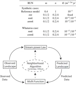
Table 1.Parameterization of the different runs
RUN m n K (m1−2 myr−1) U (m yr−1) N
total Ninit Nit
Synthetic cases:
Reference model 0.4 1 10−5 0.0005
nm 0.1/2 0.2/4 fixed fixed 22 500 5 10 000
nmk 0.1/2 0.2/4 10−6/10−4 fixed 90 000 10 30 000
unmk 0.1/2 0.2/4 10−6/10−4 0.0003/0.0008 90 000 10 30 000
Whataroa case:
nmk 0.1/2 0.2/4 10−13/10−4 fixed 90 000 10 30 000 αnmk 0.1/2 0.2/4 10−13/10−4 α: 0/1 90 000 10 30 000
Stream power Law
Observed Landscape
Predicted Landscape
Misfit Function Neighborhood
Algorithm
(Sambridge, 1999a,b)
Predicted Data Observed
Data
Figure 1. Scheme for the inversion. Observed landscape is ex-tracted from a DEM or obtained by running the SPM to steady state. The predicted landscape is obtained by running the SPL with known parameter (U, K, m and n) values selected by the NA in order to minimize the misfit function obtained by comparing the observed and predicted landscapes.
range of values makes an exhaustive search through parame-ter space a rather tedious exercise that would require a large number of forward runs. Consequently we attempted to mini-mize the computational cost by using the neighborhood algo-rithm (NA) (Sambridge, 1999a, b), an inversion method that is well adapted to solving nonlinear problems. This optimiza-tion method is based on two separate stages. The first one, called the “sampling” stage, consists in finding an ensemble of best fitting models (combinations between U, K, m and
n) that reproduce well the observed data or, in our case, that
maintain the landscape at steady state. The second one, called the “appraisal” stage, consists in deriving quantitative and statistically meaningful estimates of each parameter from the ensemble of models generated in the first stage.
In order to compare the observed or reference landscape with the predicted one, one needs to construct a misfit func-tion. In our case, we consider that both landscapes must have reached steady state (∂h/∂t=0). We use the observed or ref-erence landscape as the starting condition for the LEM to which we apply a uniform uplift increment; we then com-pute the resulting erosion over a time step of length∆t. We
define the misfit,φ, as the square root of the L2 norm of the change in height between observed hobsand predicted hpred
topographies over the time step,∆t:
φ= v u
t N
X
i=1
(hi,pred−hi,obs)2 ∆t2U2
obs
, (4)
where N is the number of pixels in the landscape. The scheme is illustrated in Fig. 1. Because Eq. (2) only applies to river profile evolution, the optimization method is applied only on river pixels and the summation in Eq. (4) is limited to the nodes that have a drainage area larger than a specified mini-mum. To normalize the misfit function, we decided not to use the error on the observed topography (as is usually the case) because this error is very small in comparison to other po-tential sources of error inherent to our assumptions of steady state and, more importantly, to the assumption that the SPL controls the evolution of stream profiles; in its place, we use the imposed or known uplift rate, U, such that the misfit be-comes a measure of the proportion of the imposed uplift rate that can be eroded back using the SPL.
To provide robust estimations of the parameter values dur-ing the appraisal stage of the inversion, the posterior prob-ability density functions (PDFs) are based on the likelihood function L, defined as
L=exp −1
2φ
2 !
. (5)
4 Application to synthetic landscapes
158 T. Croissant and J. Braun: Constraining the stream power law
Figure 2.Results from inversion for the free parameters m and n. (a) Scatter plot showing the results from NA sampling stage. (b), (c) PDFs of the two parameters resulting from the NA appraisal stage . (d) Reference model topography. (e) Topography of the best fit model. (f) Topography of a high misfit value model.
and the number of model runs. NA has a few free parameters: these are Ninit, the number of model runs in the first iteration
(i.e., for which random values of the model parameters are used), Nrunsthe number of model runs that are resampled at
each subsequent iteration (they correspond to the model runs that have given the smallest misfit value during the preceding iteration) and Nitthe number of iterations. The total number
of model runs is given by Ntot=Ninit+Nit×Nruns. The value
of each of these NA parameters is also given in Table 1. We tested various possible combinations of free param-eters (i.e., those that are tested by the inversion scheme) among n, m, K and U to see whether we could retrieve them independently of each other or whether some combinations would be better constrained than others. We present the re-sults of the following combinations:
– n and m are free, here because their ratio is supposed to
control the concavity of a river profile at equilibrium;
– n, m and K are free, here because in many circumstances
we may have independent evidence on the value of U, for example by interpreting cooling ages of rocks ob-tained by thermochronology;
– n, m, K and U are free; this would correspond to the
most common situation in natural systems.
4.1 nandmare free
In this inversion, we take for U and K the values used to cre-ate the steady-stcre-ate, reference landscape and let m and n vary freely in their preset ranges. The results of the sampling stage are shown in Fig. 2a, where each colored circle in parameter space corresponds to a model run and thus to a combination of model parameters. The color of each circle is a function of the misfit value, with the smaller misfit values correspond-ing to the warmer (red) colors. NA is designed to find the minimum value of the misfit function and converges towards
m=0.4 and n=1 (as shown also by Supplement Fig. 1), which are the values used to create the initial reference land-scape. The PDFs of each of the two parameters (Fig. 2b,c) show a narrow peak around these values, confirming that, in this configuration, we can constrain the exact value of the two parameters and a fortiori their ratio. The same result is obtained for a reference topography generated with a non-linear erosion law, i.e., n,1 (see Supplement Fig. 2) This is an interesting result that shows that if a natural landscape is at equilibrium and has been created by processes obeying the SPL exactly, and if we know the value of U and K, then we should be able to retrieve not only the value of the ra-tioθ=m/n, which has already been demonstrated to be
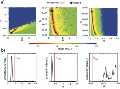
Figure 3.Results from inversion for the free parameters m, n and K. (a) Scatter plots showing the results from NA sampling stage. (b) PDFs of the three parameters resulting form the appraisal stage of NA.
4.2 n,mandKare free
In this case we assume that only the uplift rate, U, is known, and we fix it to the value used to construct the reference model by driving FastScape to steady state. The results from the sampling stage show several important points (Fig. 3a). First, the reduction of the misfit function leads to a trade-off between the m and n. All models runs that have a common
m/n ratio of 0.4 are characterized by the smallest misfit val-ues; they appear in the first panel of Fig. 3a as a red line. Note that this ratio between m and n is the same as the one used to compute the reference landscape (m/n=0.4/1.0). Second, the absolute minimum is not located at these values for m and n, as shown by the PDFs shown in Fig. 3b. Thus, if we do not know the erodibility, K, we cannot retrieve the val-ues of the m and n exponents, only their ratios as demon-strated in previous slope-area studies by Lague et al. (2000) and Snyder et al. (2000). Third, the other two scatter plots of Fig. 3a show that there is also a trade-offbetween m−n and K. The same low value of the misfit function can be achieved
with high values for K and small values of both m and n, or, conversely, with small values of K and large values of
m and n in their permissible ranges. Note that in Fig. 3, K
varies logarithmically along the vertical axis. This is eas-ily explained by the asymptotic behavior of the SPL in the
vicinity of m=n=0:
∂h
∂t =U−KA
0S0=U−K, (6)
which shows that steady state can only be reached when
K=U, where U=5×10⁻⁴is the uplift rate imposed to com-pute the steady-state reference landscape. This also explains why the optimum values of the parameters m and n obtained from the inversion are smaller than they should be (Fig. 3b and Supplement Fig. 3) – because the misfit function contains an intrinsic minimum as m and n tend toward 0. This can be illustrated by computing the difference map between the ref-erence target topography and the topography computed with various combinations of K, m and n during the inversion pro-cedure (Supplement Fig. 4), which clearly show that the dif-ference is zero when m=n=0 and K=U .
160 T. Croissant and J. Braun: Constraining the stream power law
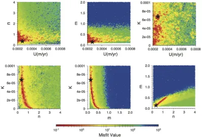
Figure 4.Results from inversion for the free parameters U, K, m and n. Scatter plots showing the results from NA sampling stage.
4.3 n,m,KandUare free
In this case, all parameters m, n, K and U are left free dur-ing the inversion. The scatter plots illustratdur-ing the behavior of the misfit function as a function of m, n and K are shown in Fig. 4 and are very similar to those of Fig. 3a. The ratio between m and n is properly retrieved and converges towards the imposed value of 0.4. The other scatter plots indicate that the uplift rate is poorly constrained and that no clear rela-tionship can be evidenced between the parameter U and the other parameters. This result clearly demonstrates that the ratioθ=m/n can indeed be constrained from a steady-state
landscape but that neither K nor U nor independent values for m and n can be constrained because of the presence of a spurious solution to the problem corresponding to m=n=0 and K=U. Moreover, if neither U nor K is constrained,
their ratio is itself unconstrained, as is the steepness index,
ks=(U/K)1/n.
We realize, however, that this result may depend on the way we have constructed the misfit function to compare the reference and predicted landscape. Other definitions of the misfit function could prove to be more constraining, espe-cially concerning the steepness index. However, if we as-sume that the shape of the reference or observed landform is the only information we possess, the definition of the misfit function we have used here makes full use of the informa-tion content of the observables, and it is difficult to see how it could be improved.
5 Application to the Whataroa catchment
5.1 Tectonic, climatic and geomorphic context
The Southern Alps, New Zealand, are the surface expres-sion of the ongoing oblique colliexpres-sion between the Australian and Pacific Plate (DeMets et al., 1990; Norris et al., 1990). This zone is characterized by very high uplift rates of up to 10 km yr−1 on the west side of the orogen (Wellman, 1979;
Tippett and Kamp, 1993; Batt et al., 2000). This results in part from the high rate of convergence between the two plates (8–12 mm yr−1) and in part from the strong orographic
con-trol on precipitations that results in precipitation rate of the order of 10–13 m yr−1on the west coast of the island, in com-parison to the much drier climate of the east coast (1 m yr−1) (Griffiths and McSaveney, 1983).
We focus our study on the Whataroa catchment (Fig. 5), which is located in the central Southern Alps along the West Coast and presents ones of the highest uplift rates in the region (≈6–8 mm yr−1) (Tippett and Kamp, 1993;
Figure 5.DEM of the Whataroa catchment in the central Southern Alps, New Zealand. AF: Alpine Fault; MD: Main Divide.
an array of braided channels during low flow periods, indicat-ing that the river is in a “transport-limited” state, i.e., trans-porting sediments eroded in the upstream part of its catch-ment towards base level.
We have used the present-day topography of the Whataroa catchment area as initial and reference landscapes in our in-version scheme. For that, we used a DEM obtained from the SRTM3 mission (resolution of 3 arcsec). We corrected it for the presence of iso-elevation areas by using the geom-etry of the current drainage system. Using ESRI ArcGIS9.3, we modified the value of each of the pixels of the DEM by an infinitesimal amount that is inversely proportional to the discharge computed by using the “real” and thus known drainage geometry. In doing so, we ensure that the discharge computed by FastScape is done in accordance with the real drainage network. We only applied the inversion procedure to the pixels that have a computed drainage area superior to a critical area of 10 km2(Supplement Fig. 5). In doing so, we impose that solely the elevation within the main river trunk and its main tributaries are used to compute the misfit func-tion. This prevents the potential bias that might be introduced by the parts of the landscape that is still glaciated and/or con-trolled by hillslope processes only. For consistency, we did not include the parts of the landscape that are below 200 m in elevation where the evolution of the landscape is likely to be transport-limited and where the SPL is unlikely to apply.
5.2 Inversion results 5.2.1 Constraint of the SPL
We applied the inversion scheme to the Whataroa catch-ment, by letting three parameters be free – m, n and K – and imposing, for each of them, a range of values that is commonly admitted in the literature (see Table 1). The Whataroa catchment is potentially ideally suited for this ex-ercise, as the lithology is relatively spatially invariant with surface rocks consisting mostly of the mildly metamor-phosed Otago schists. As the catchment is relatively small (15 km in length), it is characterized by a relatively uniform and high precipitation rate. This implies that K should be spatially uniform (∂K/∂x=0) if we neglect the effect of frac-turing. Its value is, however, poorly constrained, and we will assume that it can potentially vary by up to 9 orders of mag-nitude. We will assume that the uplift rate is well constrained by a broad range of thermochronological data to a mean value of 6 km Myr−1 (Tippett and Kamp, 1993; Batt et al.,
2000; Herman et al., 2010) and is spatially uniform. The misfit function is identical to what we used for the synthetic cases and given by Eq. (4). The values of the NA parameters
Ninit, Nitand Nrunsare given in Table 1.
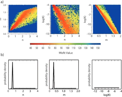
The results of the inversion (Fig. 6) show that the misfit function displays a minimum for a constant ratio between the parameters m and n in a very similar way to the results of the synthetic runs shown previously. The relationship between m and n that minimizes the misfit function is, however, not so well defined. Two peaks characterize the PDFs (Fig. 6b) for
m and n, but these values must be considered with great care
as the inversion is similarly attracted by the spurious solu-tion corresponding to m=n=0 as shown in the two panels of Fig. 6a that illustrate the behavior of the misfit function with K. It is interesting to note, however, that the optimum values for m and n – 0.3 and 0.5, respectively – are somewhat different from the extremum values allowed by the imposed ranges (0.2<m<1.5 and 0.4<n<2.5), which could sug-gest that these values are potentially meaningful. Regardless of these considerations, it is the ratio of the two exponents, i.e., the concavity, that is best constrained at a value of 0.6. Similar to the synthetic cases, no constraint can be obtained for the value of K, as illustrated by the PDF of this parameter in the last panel of Fig. 6b.
As in the synthetic cases, the optimization method proves to be efficient in constraining the ratio m/n. For the Whataroa
catchment and under the assumption that it is in geomorphic steady state, the optimum value is found to be 0.6, which sits within the range of acceptable values but towards their upper bound.
5.2.2 Constraint on the uplift geometry
162 T. Croissant and J. Braun: Constraining the stream power law
Figure 6.Results from inversion for the free parameters K, m and n. (a) Scatter plots showing the results from NA sampling stage. (b) PDFs of the three parameters resulting form the appraisal stage of NA.
Low-temperature thermochronology data from rocks ex-posed along the western side of the Southern Alps are com-monly interpreted as evidence for an increase in exhuma-tion rate towards the Alpine Fault (Tippett and Kamp, 1993). Higher temperature thermochronological data as well as first-order structural evidence that all of the structures east of and including the Alpine Fault are east-dipping reverse faults im-ply that the uplift and exhumation rates should be maximum near the present-day divide and thus decrease towards the Alpine Fault (Braun et al., 2010).
In order to test these two hypotheses, we allowed the up-lift rate to vary linearly between the base of the Whataroa catchment near the Alpine Fault and the position of the main divide at the top of the catchment in such a way that either of the two scenarios can be reproduced by varying a single coefficient,α, introduced in the definition of the uplift rate function, U(x):
U=2(1−α)U0(1− x
L)+2αU0 x
L, (7)
where U0 the mean uplift rate in the Whataroa catchment
(6 km Myr−1), L the distance between the Alpine Fault and
the Main Divide and x the position varying between 0 and L. In this expression,αvaries between 0 and 1 corresponding to
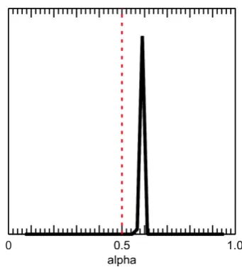
a maximum uplift rate near the Alpine Fault or the Main Di-vide, respectively (Fig. 7);α=0.5 corresponds to a spatially uniform uplift rate.
In the following inversion, four parameters were left free:
how-AF MD
AF MD
AF MD
α = 0
α = 0.5
α = 1
Figure 7.Three extreme cases controlled by the value ofα. AF: Alpine Fault; MD: Main Divide.
ever, about applying a similar treatment to K as we did for
U, i.e., allowing it to vary linearly as a function to the Alpine
Fault, as we have no hard constraint on its mean value, nor on how it may depend on fracturing. This implies that we would need to introduce two free parameters to represent a spatial variation in K, while we have shown that a single value can-not be constrained from topographic data only.
6 Discussion
6.1 Steady-state assumption
How to define whether a mountain range has reached steady state has been the object of numerous studies (Braun and Sambridge, 1997; Willett et al., 2001; Willett and Brandon, 2002), mostly based on the use of SPMs. True topographic steady state is reached when each point of the landscape re-mains at a constant elevation with respect to base level. Al-though such a situation might be achieved in a numerical model, whether it can be or has even been reached in a natural system remains difficult to imagine. One of the main reasons is that the horizontal advection of landforms prevents erosion and uplift rates from perfectly compensating each other on an orogenic scale (Willett et al., 2001). Better questions to ask might be on which spatial scale can we expect geomorphic steady state to develop and over which time frame.
The work we presented here is based on the assumption that geomorphic systems do reach steady state and that it has been reached in at least some parts of the Southern Alps in New Zealand. Under this assumption, the optimization scheme we have developed show that one can constrain the parameterization of channel incision from the geometry of the steady-state landscape. However, these constraints are
Figure 8.Results from inversion: PDF of the parameterα.
relatively weak and do not permit considering the SPL as a predictive tool, i.e., a law that could be transposed to a range of environments in a physically consistent manner.
To improve our method and extract more useful constraints on the SPL parameterization, we need to relax our hypothe-sis of steady state, which will imply longer, more computer-intensive simulations. We are in the process of doing so, but, concomitantly, we will need to find and utilize observational constraints on the time evolution of the system. Otherwise, simulating or predicting the rate of evolution of a landform from its shape only, and thus without a priori knowledge or independent constraints on uplift rate or the rate of landform evolution, is a futile exercise and therefore certain to fail.
6.2 Comparison to other studies
The use of optimization methods has been rather limited in geomorphology, mostly due to the long computational times required to run SPMs at the required resolution. Most pre-vious attempts were limited to fitting 1-D longitudinal river profiles (van Der Beek and Bishop, 2003; Tomkin et al., 2003; Roberts and White, 2010) or to systematic search through low-dimension parameter search (van der Beek and Braun, 1998).
164 T. Croissant and J. Braun: Constraining the stream power law
values for the model parameters, which, they noted, are strongly controlled by lithology.
More recent studies have attempted to deduce uplift rate histories from longitudinal river profiles (Roberts and White, 2010; Roberts et al., 2012). In these studies, the SPL coeffi -cients were derived from independent constraints (minimum residual misfit between theoretical observed and river pro-files for m and n, and local incision estimate and known uplift histories for K) and used to both derive a simple relationship and reproduce knickpoint propagation. The two main loca-tions where they have applied this method (Africa and the Colorado Plateau) have not been affected by recent tectonic events and their recent uplift history is assumed to be related to mantle processes (mantle plume impinging on the over-lying lithosphere or dynamic topography caused by mantle circulation), implying that the inversion scheme must be per-formed over relatively long periods of time (i.e., 50 Myr). This approach neglects lithological control on knickpoint propagation and potential variations in climate (precipita-tion) and/or catchment geometry, which is difficult to justify over such long periods of time. Although Roberts and White (2010) and Roberts et al. (2012) do not explicitly aim at con-straining the SPL coefficients, their studies demonstrate that present-day river profiles can be reproduced with great accu-racy using arbitrarily defined model parameters and therefore do not contain all the information necessary to constrain the SPL parameterization.
The study we present here is the first that considers the problem in 2-D and lets the SPL coefficients vary over broad ranges in order to determine their best values in a quantita-tive manner. We also show that the method is able to retrieve information about the distribution of present-day uplift, even under the assumption of geomorphic steady state.
6.3 The stream power law
Although the SPL used in this study is able to reproduce many observations and natural processes (i.e., the concav-ity of river profiles to the migration of knickpoints), it must be regarded as a first-order parameterization of the integrated effects of river incision and, as such, cannot be expected to adequately represent the many and varied physical processes at play. For example, the SPL cannot include the effect of sediment being delivered to the river channel by hill-slope processes. In most of the Whataroa catchment, which is sub-jected to rapid tectonic uplift, valley sides are at the critical angle of repose, as indicated by their steep, V-shaped mor-phology (Herman and Braun, 2006) and supply vast quantity of sediments to the streams. Several formulations have been proposed to include the effect of sediment (both bed load and suspended load) on the erosional power of a stream, its trans-port capacity and the way sediment protects the bed from erosion (Beaumont et al., 1992; Sklar and Dietrich, 2001). Furthermore, tectonic uplift is accompanied by deformation and fracturing, which is clearly evidenced by the intense
hy-drothermal activity in the vicinity of the Alpine Fault (Allis and Shi, 1995). The resistance of rocks to erosion is very likely to be strongly influenced by fracturing (Molnar et al., 2007), but it cannot be included in the SPL in a physically meaningful manner; at best the coefficient K can be arbitrar-ily adjusted to represent the zeroth-order effect of fracturing on erodibility.
In most of our inversions, the minimum misfit value re-mains quite high, which could lead to one of two conclu-sions: that (a) the classical formulation of the SPL used here is not sufficiently complex to reproduce a steady-state land-scape or (b) that geomorphic steady state does not exist or does not apply to the Whataroa catchment. Further investiga-tion is required to determine whether introducing a better pa-rameterization of channel width, the effect of sediment load on the incision power of a stream in the SPL or spatial varia-tions in K related to lithology or precipitation patterns would lead to a substantial reduction in misfit.
Progressing in the testing and improving of stream incision laws also requires that we go beyond fitting topographic data and introduce in our inversions observational evidence on the temporal evolution of a stream profile. This includes a broad range of thermochronometric tools as well as exposure dating techniques. Sediment provenance data are another important tool that should provide independent information to constrain the SPL (or other potential parameterizations).
7 Conclusions and perspectives
We have presented here a novel approach to constrain the coefficients of the SPL parameters that combines a very ef-ficient surface process model (FastScape) and an inversion method (the neighborhood algorithm). The inversion is con-strained by a misfit function that compares a reference or ob-served topography with that predicted by the SPM under the assumption of geomorphic steady state. Using the method on synthetic landscapes, we have demonstrated its potential by an in-depth analysis of the resulting misfit function that is dependent on the number of degrees of freedom (or model parameters) in the inversion procedure. We proved that the method is accurate and efficient to retrieve the ratio between
m and n, the two exponents in the SPL formulation, that
strongly controls the concavity of river profiles.
We applied the method to a natural landscape from the South Island of New Zealand where geomorphic steady state is likely to be achieved due to the present-day, very high tec-tonically driven uplift rates. In this case, we show that the ratio m/n can be constrained but that the estimate we obtain
is close to the upper bound of commonly “accepted” values, suggesting that the region may be subject to substantial spa-tial variations in uplift rate. We also show that the value of none of the SPL coefficients can be retrieved with confidence due to the presence of a spurious solution corresponding to
We also performed an inversion in which uplift rate was allowed to vary spatially around a fixed mean value that is relatively well constrained in New Zealand through the inter-pretation of many thermochronological data sets. The results show that the preferred solution (i.e., the one that minimizes the misfit between observed and predicted elevation) implies a decrease in uplift rate towards the Alpine Fault, which is consistent with a recent study demonstrating that the strong gradient in deformation east of the Alpine Fault indicates that uplift rate must increase with distance from the Alpine Fault (Braun et al., 2010).
We also conclude that although promising, the method we have developed needs to be improved to include transient ef-fects, other observational constraints on the temporal evolu-tion of landscapes, and the spatial distribuevolu-tion of erosion rate in and out of the channels, which will also require modifica-tion of the misfit funcmodifica-tion.
Supplementary material related to this article is available online at http://www.earth-surf-dynam.net/2/ 155/2014/esurf-2-155-2014-supplement.pdf.
Acknowledgements. The authors wish to thank the Institut Universitaire de France for funding T. C. MSc stipend and Dimitri Lague for constructive comments on an earlier version of this manuscript. We are grateful to G. R. Roberts and A. Howard, whose comments helped to improve the manuscript. M. Sambridge is thanked for making the neighborhood algorithm code available.
Edited by: S. Castelltort
References
Adams, J.: Contemporary uplift and erosion of the Southern Alps, New Zealand, Geol. Soc. Am. Bull., 91, 1–114, 1980.
Allis, R. and Shi, Y.: New insights into temperature and pressure beneath the central Southern Alps, New Zealand, New Zealand, J. Geol. Geophys., 38, 585–592, 1995.
Batt, G. E., Braun, J., Kohn, B. P., and McDougall, I.: Ther-mochronological analysis of the dynamics of the Southern Alps, New Zealand, Geol. Soc. Am. Bull., 112, 250–266, 2000. Beaumont, C., Fullsack, P., and Hamilton, J.: Erosional control of
active compressional orogens, in: Thrust Tectonics, edited by McClay, K. R., pp. 1–18, Chapman and Hall, New York, 1992. Braun, J. and Sambridge, M.: Modelling landscape evolution on
ge-ological time scales: a new method based on irregular spatial dis-cretization, Basin Research, 9, 27–52, 1997.
Braun, J. and Willett, S. D.: A very efficient O (n), implicit and parallel method to solve the stream power equation governing fluvial incision and landscape evolution, Geomorphology, 180– 181, 170–179, 2013.
Braun, J., Herman, F., and Batt, G.: Kinematic strain localization, Earth Planet. Sci. Lett., 300, 197–204, 2010.
Crave, A. and Davy, P.: A stochastic precipiton model for simulating erosion/sedimentation dynamics, Computers Geosci., 27, 815– 827, 2001.
DeMets, C., Gordon, R. G., Argus, D. F., and Stein, S.: Current plate motions, Geophys. J. Internat., 101, 425–478, 1990.
Duvall, A., Kirby, E., and Burbank, D.: Tectonic and litho-logic controls on bedrock channel profiles and processes in coastal California, J. Geophys. Res. (2003–2012), 109, doi: 10.1029/2003JF000086, 2004.
Griffiths, G. A. and McSaveney, M. J.: Distribution of mean annual precipitation across some steepland regions of New Zealand., N. Z. J. SCI., 26, 197–209, 1983.
Herman, F. and Braun, J.: Fluvial response to horizontal shortening and glaciations: A study in the Southern Alps of New Zealand, J. Geophys. Res. (2003–2012), 111, doi: 10.1029/2004JF000248, 2006.
Herman, F., Rhodes, E. J., Braun, J., and Heiniger, L.: Uni-form erosion rates and relief amplitude during glacial cycles in the Southern Alps of New Zealand, as revealed from OSL-thermochronology, Earth Planet. Sci. Lett., 297, 183–189, 2010. Howard, A. D.: A detachment-limited model of drainage basin
evo-lution, Water resources research, 30, 2261–2285, 1994. Kirby, E. and Whipple, K. X.: Quantifying differential rock-uplift
rates via stream profile analysis, Geology, 29, 415–418, 2001. Kirby, E. and Whipple, K. X.: Expression of active tectonics in
ero-sional landscapes, J. Struct. Geol., 44, 54–75, 2012.
Kooi, H. and Beaumont, C.: Escarpment evolution on high-elevation rifted margins: Insights derived from a surface pro-cesses model that combines diffusion, advection, and reaction, J. Geophys. Res. (1978–2012), 99, 12191–12209, 1994. Lague, D., Davy, P., and Crave, A.: Estimating uplift rate and
erodi-bility from the area-slope relationship: Examples from Brittany (France) and numerical modelling, Phys. Chem. Earth, Part A, 25, 543–548, 2000.
Molnar, P., Anderson, R., and Anderson, S.: Tectonics, fractur-ing of rock, and erosion, J. Geophys. Res., 112, F03014, doi: 10.1029/2005JF000433, 2007.
Montgomery, D. R. and Brandon, M. T.: Topographic controls on erosion rates in tectonically active mountain ranges, Earth Planet. Sci. Lett., 201, 481–489, 2002.
Norris, R. J., Koons, P. O., and Cooper, A. F.: The obliquely-convergent plate boundary in the South Island of New Zealand: implications for ancient collision zones, J. Struct. Geol., 12, 715– 725, 1990.
Roberts, G. G. and White, N.: Estimating uplift rate histories from river profiles using African examples, J. Geophys. Res., 115, B02406, doi: 10.1029/2009JB006692, 2010.
Roberts, G. G., White, N. J., Martin-Brandis, G. L., and Crosby, A. G.: An uplift history of the Colorado Plateau and its surround-ings from inverse modeling of longitudinal river profiles, Tecton-ics, 31, TC4022, doi: 10.1029/2012TC003107, 2012.
Sambridge, M.: Geophysical Inversion with a neibourhood algo-rithm – I. Searching a parameter space, Geophys. J. Int., 138, 479–494, 1999a.
Sambridge, M.: Geophysical Inversion with a neibourhood algo-rithm – II. Appraising the ensemble, Geophys. J. Int., 138, 727– 746, 1999b.
166 T. Croissant and J. Braun: Constraining the stream power law
Sklar, L. and Dietrich, W. E.: River longitudinal profiles and bedrock incision models: Stream power and the influence of sed-iment supply, GEOPHYSICAL MONOGRAPH-AMERICAN GEOPHYSICAL UNION, 107, 237–260, 1998.
Snyder, N. P., Whipple, K. X., Tucker, G. E., and Merritts, D. J.: Landscape response to tectonic forcing: Digital elevation model analysis of stream profiles in the Mendocino triple junction re-gion, northern California, Geological Society of America Bul-letin, 112, 1250–1263, 2000.
Stock, J. D. and Montgomery, D. R.: Geologic constraints on bedrock river incision using the stream power law, J. Geophys. Res. (1978–2012), 104, 4983–4993, 1999.
Tippett, J. M. and Kamp, P. J. J.: Fission track analysis of the late Cenozoic vertical kinematics of continental Pacific crust, South Island, New Zealand, J. Geophys. Res., 98, 16119–16148, 1993. Tomkin, J. H., Brandon, M. T., Pazzaglia, F. J., Barbour, J. R., and Willett, S. D.: Quantitative testing of bedrock incision models for the Clearwater River, NW Washington State, J. Geophys. Res., 108, 2308, doi: 10.1029/2001JB000862, 2003.
Tucker, G., Lancaster, S., Gasparini, N., and Bras, R.: The channel-hillslope integrated landscape development model (CHILD), in: Landscape erosion and evolution modeling, Springer, 349–388, 2001.
Tucker, G. E. and Hancock, G. R.: Modelling landscape evolution, Earth Surf. Proc. Land., 35, 28–50, 2010.
Van Der Beek, P. and Bishop, P.: Cenozoic river profile development in the Upper Lachlan catchment (SE Australia) as a test of quan-titative fluvial incision models, J. Geophys. Res. (1978–2012), 108, doi:10.1029/2002JB002125, 2003.
van der Beek, P. and Braun, J.: Numerical modelling of landscape evolution on geological time-scales: a parameter analysis and comparison with the south-eastern highlands of Australia, Basin Research, 10, 49–68, 1998.
Wellman, H. W.: An uplift map for the South Island of New Zealand, and a model for uplift of the Southern Alps, Bull. R. Soc. NZ, 18, 13–20, 1979.
Whipple, K. X.: Bedrock rivers and the geomorphology of active orogens, Annu. Rev. Earth Planet. Sci., 32, 151–185, 2004. Whipple, K. X. and Tucker, G. E.: Dynamics of the stream-power
river incision model: Implications for height limits of mountain ranges, landscape response timescales, and research needs, J. Geophys. Res., 104, 17661–17674, 1999.
Whittaker, A. C., Cowie, P. A., Attal, M., Tucker, G. E., and Roberts, G. P.: Bedrock channel adjustment to tectonic forc-ing: Implications for predicting river incision rates, Geology, 35, 103–106, 2007.
Willett, S. D. and Brandon, M. T.: On steady states in mountain belts, Geology, 30, 175–178, 2002.