https://doi.org/10.5194/cp-13-1695-2017 © Author(s) 2017. This work is distributed under the Creative Commons Attribution 3.0 License.
Simulation of climate, ice sheets and CO
2
evolution
during the last four glacial cycles with an Earth system
model of intermediate complexity
Andrey Ganopolski1and Victor Brovkin2,a
1Potsdam Institute for Climate Impact Research (PIK), Potsdam, Germany 2Max Plank Institute for Meteorology, Hamburg, Germany
aalso a guest scientist at: Potsdam Institute for Climate Impact Research (PIK), Potsdam, Germany
Correspondence to:Andrey Ganopolski ([email protected])
Received: 27 March 2017 – Discussion started: 19 April 2017
Revised: 15 September 2017 – Accepted: 9 October 2017 – Published: 29 November 2017
Abstract. In spite of significant progress in paleoclimate reconstructions and modelling of different aspects of the past glacial cycles, the mechanisms which transform regional and seasonal variations in solar insolation into long-term and global-scale glacial–interglacial cycles are still not fully understood – in particular, in relation to CO2 variability. Here using the Earth system model of intermediate com-plexity CLIMBER-2 we performed simulations of the co-evolution of climate, ice sheets, and carbon cycle over the last 400 000 years using the orbital forcing as the only ex-ternal forcing. The model simulates temporal dynamics of CO2, global ice volume, and other climate system character-istics in good agreement with paleoclimate reconstructions. These results provide strong support for the idea that long and strongly asymmetric glacial cycles of the late Quater-nary represent a direct but strongly nonlinear response of the Northern Hemisphere ice sheets to orbital forcing. This re-sponse is strongly amplified and globalised by the carbon cy-cle feedbacks. Using simulations performed with the model in different configurations, we also analyse the role of indi-vidual processes and sensitivity to the choice of model pa-rameters. While many features of simulated glacial cycles are rather robust, some details of CO2evolution, especially during glacial terminations, are sensitive to the choice of model parameters. Specifically, we found two major regimes of CO2changes during terminations: in the first one, when the recovery of the Atlantic meridional overturning circula-tion (AMOC) occurs only at the end of the terminacircula-tion, a pronounced overshoot in CO2concentration occurs at the be-ginning of the interglacial and CO2remains almost constant
during the interglacial or even declines towards the end, re-sembling Eemian CO2dynamics. However, if the recovery of the AMOC occurs in the middle of the glacial termination, CO2 concentration continues to rise during the interglacial, similar to the Holocene. We also discuss the potential con-tribution of the brine rejection mechanism for the CO2 and carbon isotopes in the atmosphere and the ocean during the past glacial termination.
1 Introduction
forc-ing. This fact strongly suggests an opposite interpretation of close correlation between global ice volume and CO2during Quaternary glacial cycles – namely that glacial cycles rep-resent a strongly nonlinear response of the Earth system to the orbital forcing (Paillard, 1998), while variations in CO2 concentration are directly driven by ice sheet fluctuations. In turn, CO2variations additionally strongly amplify and glob-alise the direct response of ice sheets to the orbital forcing.
In spite of the significant number of studies aimed at ex-plaining low glacial CO2concentrations (e.g. Archer et al., 2000; Sigman and Boyle, 2000; Watson et al., 2000), the influence of ice sheets on the carbon cycle remains poorly understood. It is also unclear the extent to which CO2 varia-tions represent a direct response to ice sheet forcing and how much is the result of additional amplification of CO2 vari-ations through the climate–carbon cycle feedback. Indeed, although radiative forcing of ice sheets contributes about 50 % to glacial–interglacial variations in global temperature (Brady et al., 2013), most of the cooling associated with ice sheets is restricted to the area covered by ice sheets and their close proximity. Thus, the direct contribution of ice sheets to glacial ocean cooling is rather limited, and therefore the ef-fect of ice sheets on CO2 drawdown through the solubility effect can explain only a fraction of the reduction in glacial CO2. At the same time, the direct effect of ice sheets on at-mospheric CO2concentration through ca. 3 % changes in the ocean volume and global salinity is rather well understood but works in the opposite direction and leads to a glacial CO2 rise of about 10–20 ppm (Sigman and Boyle, 2000; Brovkin et al., 2007). Another direct effect of ice sheet growth on the carbon cycle through reducing the area covered by forest (e.g. Prentice et al., 2011) also operates in the opposite direc-tion. However, several other processes could potentially con-tribute to glacial CO2 drawdown through ice sheet growth and related lowering of sea level. One such mechanism is enhanced biological productivity in the Southern Ocean due to the iron fertilisation effect (Martin, 1990; Watson et al., 2000). The latter is attributed to enhanced dust deposition over the Southern Ocean seen in the paleoclimate records (Martinez-Garcia et al., 2014; Wolff et al., 2006). At least part of this enhanced deposition is associated with the dust mobilisation from exposed Patagonian shelf and glaciogenic dust production related to the Patagonian ice cap (Mahowald et al., 1999; Sugden et al., 2009). A number of studies on the effect of iron fertilisation suggested a contribution of 10 to 30 ppm to the glacial CO2decrease (e.g. Watson et al., 2000; Brovkin et al., 2007). Another effect is related to the brine re-jection mechanism, more specifically, to a much deeper pen-etration of brines produced during sea ice formation in the Southern Ocean during glacial time. The latter is explained by shallowing and significant reduction of the Antarctic Shelf area. According to Bouttes et al. (2010) this mechanism, in combination with enhanced stratification of the deep ocean, can contribute up to 40 ppm to the glacial CO2lowering.
Apart from the mechanisms mentioned above, many other processes have been proposed to explain low glacial CO2 concentration. Among them are changes in the ocean cir-culation (Watson et al., 2015) and an increase in Southern Ocean stratification (e.g. Kobayashi et al., 2015), increase in sea ice area in the Southern Ocean (Stephens and Keel-ing, 2000) and a shift in the westerlies (Toggweiler et al., 2006), increase in nutrient inventory or change in the marine biota stoichiometry (Sigman and Boyle, 2000; Wallmann et al., 2016), changes in coral reefs accumulation and disso-lution (Opdyke and Walker, 1992), accumulation of carbon in the permafrost regions (Ciais et al., 2012; Brovkin et al., 2016), variable volcanic outgassing (Huybers and Langmuir, 2009), and several other mechanisms. Most of these pro-cesses are not directly related to ice sheet area or volume, and thus should be considered as amplifiers or modifiers of the direct response of CO2 to ice sheets operating through the climate–carbon cycle feedbacks. Although paleoclimate records provide some useful constraints, the relative role of particular mechanisms at different stages of glacial cycles re-mains poorly understood.
Most studies of glacial–interglacial CO2 variations per-formed to date have been aimed at explaining the low CO2 concentration at the Last Glacial Maximum (LGM, ca. 21 ka). In these studies, both continental ice sheets and the radiative forcing of low glacial CO2concentration were pre-scribed from paleoclimate reconstructions. Only a few have attempted to explain CO2dynamics during a part of (usually the glacial termination) or the entire last glacial cycle, with models of varying complexity – from simple box-type els (e.g. Köhler et al., 2010; Wallmann et al., 2016), to mod-els of intermediate complexity (Brovkin et al., 2012; Men-viel et al., 2012), or a stand-alone complex ocean carbon cy-cle model (Heinze et al., 2016). In all these studies, radia-tive forcing of CO2 (or total GHGs) was prescribed based on paleoclimate reconstructions. Similarly, ice sheets’ dis-tribution and elevation were derived from paleoclimate re-constructions or model simulations where radiative forcing of GHGs has been prescribed. Thus, in all these studies, CO2 was treated as an external forcing rather than an internal feed-back. Here we for the first time perform simulations of the Earth system dynamics during the past four glacial cycles using fully interactive ice sheet and carbon cycle modelling components, and therefore the only prescribed forcing in this experiment is the orbital forcing.
2 The model and experimental setup
2.1 CLIMBER-2 model description
ice model, the three-dimensional thermomechanical ice sheet model SICOPOLIS (Greve, 1997), the dynamic model of the terrestrial vegetation VECODE (Brovkin et al., 1997), and the global carbon cycle model (Brovkin et al., 2002, 2007). Atmosphere and ice sheets are coupled bidirectionally us-ing a physically based energy balance approach (Calov et al., 2005). The ice sheet model is only applied to the North-ern Hemisphere. The contribution of the Antarctic ice sheet to global ice volume change is assumed to be constant dur-ing glacial cycles and equal to 10 %. The model also in-cludes parameterisation of the impact of aeolian dust depo-sition on snow albedo (Calov et al., 2005; Ganopolski et al., 2010). The CLIMBER-2 model in different configurations has been used for numerous studies of past and future cli-mates – in particular, simulations of glacial cycles (Ganopol-ski et al., 2010, 2016; Ganopol(Ganopol-ski and Calov, 2011; Willeit et al., 2015) and carbon cycle operation during the last glacial cycle (Brovkin et al., 2012).
As has been shown by Ganopolski and Roche (2009), the temporal dynamics of the Atlantic meridional over-turning circulation (AMOC) during glacial terminations in CLIMBER-2 are very sensitive to the magnitude of fresh-water flux to the North Atlantic. To explore different possi-ble deglaciation evolutions, together with the standard model version, we performed an additional suite of simulations, in which the component of freshwater flux into the ocean originated from melting of ice sheets was uniformly scaled up or down by up to 10 %. This rather small change in the freshwater forcing (typically smaller than 0.02 Sv) does not affect AMOC dynamics appreciably most of the time but does induce a strong impact during deglaciations (see below). Other modifications of the climate–ice-sheet component of the model are described in the Appendix.
The ocean carbon cycle model includes modules for ma-rine biota, oceanic biogeochemistry, and deep ocean sedi-ments. Biological processes in the euphotic zone (the upper 100 m in the model) are explicitly resolved using the model for plankton dynamics by Six and Maier-Reimer (1996). The sediment diagenesis model (Archer, 1996; Brovkin et al., 2007) calculates burial of CaCO3in the deep sea, while shallow-water CaCO3 sedimentation is simulated based on the coral reef model (Kleypas, 1997) driven by sea level change. Silicate and carbonate weathering rates are scaled to the runoff from the land surface; they are also affected by sea level change (Munhoven, 2002). Compared to Brovkin et al. (2012), the carbon cycle model has been modified in sev-eral aspects. Similar to Brovkin et al. (2012), the efficiency of nutrient utilisation in the Southern Ocean is set to be pro-portional to the dust deposition rate (see Appendix), which in the case of one-way coupling is prescribed to be propor-tional to the dust deposition in the EPICA ice core. However, in the fully interactive experiment, the dust deposition rate over the Southern Ocean has been computed from simulated sea level (see Appendix). This means that in the fully inter-active experiments (see below) we did not explicitly use any
paleoclimate data to drive the model, and the orbital forcing was the only prescribed forcing. In the marine carbon cycle component, we also account for a dependence of the reminer-alisation depth on ocean temperature following Segschneider and Bendtsen (2013) (see Appendix). In our previous studies the remineralisation depth was kept constant.
The CLIMBER-2 model used in earlier studies of glacial carbon cycle did not include long-term terrestrial carbon pools such as permafrost carbon, peat, and carbon buried be-neath the ice sheets. In the present version of the model, these pools are included. The model also accounts for peat accu-mulation. Modification of the terrestrial carbon cycle compo-nents is described in detail in the Appendix. For simulation of atmospheric radiocarbon during the last glacial termina-tion we used the rate of14C production following the sce-nario of Hain et al. (2014), which is based on the production model of Kovaltsov et al. (2012).
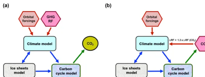
Figure 1.Coupling strategy.(a)One-way coupled experiment;(b)fully interactive experiment.
both types of experiments were obtained identically to Calov et al. (2005) and Ganopolski and Calov (2011) by scaling the fields computed with global climate models, where the scal-ing parameter was proportional to the global ice volume.
2.3 Model spin-up
The model spin-up and the proper choice of model param-eters for simulation of multiple glacial cycles represent a challenge when using the model with long-term components of the carbon cycle because inconsistent initial conditions or even a small imbalance in carbon fluxes could lead to a large drift in simulated atmospheric CO2 concentration (in the case of one-way coupling) or the state of the entire Earth system (climate, ice sheets, CO2) in the case of the fully in-teractive experiments. Note that, in the latter case, the neg-ative climate–weathering feedback will eventually stabilise the system but this occurs at a timescale of several glacial cy-cles and over this time climate could drift far away from its realistic state. To avoid such drift, volcanic outgassing should be carefully calibrated. Based on a set of sensitivity experi-ments, we found that the value of 5.3 Tmol C yr−1allows us to simulate quasiperiodic cycles without a long-term trend in atmospheric CO2. Note that even a±10 % change in volcanic outgassing leads to a significant (order of 100 ppm) drift in CO2concentration simulated over the last four glacial cycles. When the carbon cycle model incorporates such long-term processes as terrestrial weathering, marine sediment accumu-lation, and permafrost carbon burial, the assumption that the system is close to equilibrium at the pre-industrial period or at any other moment of time is not valid even if the CO2 concentration was relatively stable during a certain time in-terval. To produce proper initial conditions at 410 ka we per-formed a sequence of 410 kyr long one-way coupled runs with the identical forcings. In the first run we used as the ini-tial conditions the final state obtained in simulation of the last glacial cycles (Brovkin et al., 2012). Then we launched each 410 kyr experiment from the final state obtained in the previ-ous model run. The results of such sequence of experiments reveal a clear tendency to converge to the solution with sim-ilar initial and final states of the Earth system. We then used
the state of climate and carbon cycle obtained at the end of the last run as the initial conditions for all experiments pre-sented in this paper. In the analysis of all experiments de-scribed below, we exclude the first 10 000 years.
3 Simulations of the last four glacial cycles
Realistic simulation of climate and carbon cycle evolution during the last four glacial cycles is more challenging in the case of the fully interactive configuration, because in this case a number of additional positive feedbacks tend to am-plify initial model biases. Therefore we begin our analysis with the one-way coupled simulations similar to that per-formed in Brovkin et al. (2012). This configuration was also used for the calibration of new parameterisations (see Sect. 4) and a set of sensitivity experiments for the last glacial termi-nation (Sect. 5).
3.1 Experiments with one-way coupled climate–carbon cycle model
Simulated climate and ice sheet variations in the one-way coupled experiments are similar to the ones presented in Ganopolski and Calov (2011), which is not surprising since the only difference between model versions used in these studies is related to the coupling between ice sheet and cli-mate components (see Appendix). Simulated glacial cycles are characterised by global surface air temperature variations of about 5◦C (not shown) and maximum sea level drops by more than 100 m during several glacial maxima. Simulated global ice sheet volume most of the time is close to the re-constructed one (Spratt and Lisiecki, 2016) (Fig. 2d). In gen-eral, differences between simulated and reconstructed global sea level are comparable to the uncertainties in sea level re-constructions obtained using different methods.
(a)
(b)
(c)
(d)
(e)
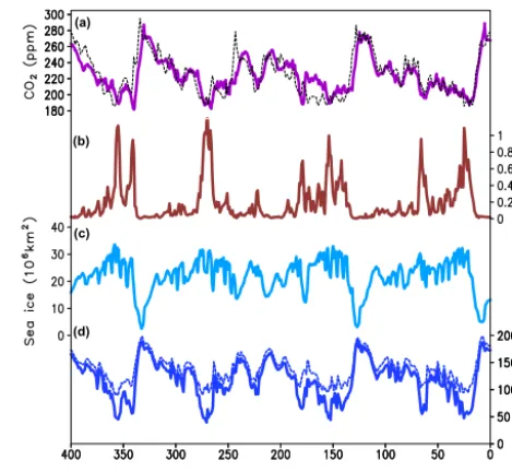
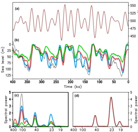
Figure 2.Transient simulations of the last four glacial cycles forced by orbital variations, observed concentration of well-mixed GHGs, and dust deposition rate (one-way coupled experiments).(a) Maxi-mum summer insolation at 65◦N, W m−2;(b)radiative forcing (rel-ative to pre-industrial) of well-mixed GHGs, W m−2;(c) Antarc-tic dust deposition rate in relative units;(d)global ice volume ex-pressed in sea level equivalent (m);(e)atmospheric CO2 concen-tration (ppm). Dark red colour in(a)–(c)represents prescribed forc-ings. Black dashed line in(d)is the sea level stack from Spratt and Lisiecki (2016), and in (e)is the compiled Antarctic CO2 record
from Lüthi et al. (2008). Radiative forcing of GHGs in(b)is from Ganopolski and Calov (2011). Antarctic dust is from Augustin et al. (2004). Blue lines in(d, e)correspond to the baseline experiment ONE_1.0 and purple lines to experiment ONE_1.1, where meltwa-ter flux into the Atlantic was scaled up by a factor of 1.1.
model version (ONE_1.0) and model with 10 % enhanced meltwater flux (ONE_1.1) are essentially identical most of the time, except for glacial terminations. During glacial ter-minations even small differences in the freshwater forcing cause pronounced differences in the temporal evolution of the AMOC, and as a result, of CO2concentration. As seen in Fig. 2d, in the experiment ONE_1.0, CO2 concentration grows monotonically during the last glacial termination (TI, midpoint at ca. 15 ka) and Termination IV (ca. 330 ka) while it rises faster and overshoots the interglacial level during Ter-minations II (ca. 135 ka) and III (ca. 240 ka). In contrast, in experiment ONE_1.1, similar overshoots occur during Ter-minations I and III but not Termination IV. In all cases,
sim-Figure 3. Temporal evolution of the AMOC, Sv(a), and atmo-spheric CO2concentration, ppm(b)during the last four glacial
ter-minations. Blue lines correspond to experiment ONE_1.0 and pur-ple lines to experiment ONE_1.1, where meltwater flux into the At-lantic was scaled up by a factor of 1.1.
ulated CO2lags behind the reconstructed one but this lag is smaller in the cases when overshoot is simulated. Experi-ments with CO2overshoots are clearly in better agreement with empirical data for MIS7 and MIS9. Analysis of model results shows that pronounced CO2overshoot occurs in the case when the AMOC is suppressed during the entire glacial termination and recovers only after the cessation of meltwa-ter flux (Fig. 3). In contrast, if the AMOC recovers well be-fore the end of deglaciation, simulated CO2experiences only local overshoot and continues to rise during most of the inter-glacial. The latter behaviour is similar to that was observed in reality during MIS11 and the Holocene, while the former is typical for MIS5, 7, and 9. Thus our model is able to repro-duce both types of CO2dynamics during recent interglacials. The rise of CO2 by 10–20 ppm on the millennial timescale during AMOC shutdowns is a persistent feature of CLIMBER-2 and the mechanism of this rise has been ex-plained in Brovkin et al. (2012) by a weakening of the reverse cell of the Indo-Pacific overturning circulation during peri-ods of reduced AMOC. A similar rise in atmospheric CO2 concentration during periods of AMOC shutdown has been simulated in some other (but not all) similar modelling ex-periments. Incorporation of the temperature-dependent rem-ineralisation depth additionally contributes to the CO2 over-shoots at the beginning of several interglacials (see below) but the mechanism described in Brovkin et al. (2012) remains the dominant one.
(a)
(b)
(c)
(d)
Figure 4. Simulated CO2 and δ13C with the one-way coupled
model (ONE_1.0).(a)CO2concentration (ppm) (Lüthi et al, 2008)
(b) atmosphericδ13CO2(‰),(c)deep South Atlanticδ13C (‰);
(d)deep North Pacificδ13C (‰). Colour lines – model results. Em-pirical data (black dashed lines):(a)Lüthi et al. (2008);(b) Eggle-ston et al. (2016);(c, d)Lisiecki et al. (2008).
simulated and reconstructed (Eggleston et al., 2016) atmo-sphericδ13CO2is rather poor. Both model and data show a drop in atmosphericδ13CO2during the last and penultimate deglaciations but the data also suggest the strong drop at the end of Eemian interglacial while the model simulated a con-tinuous rise ofδ13CO2during this interval. In addition, tem-poral variability of the reconstructedδ13CO2is significantly larger than the simulated one. A more detailed comparison with empirical data during the last deglaciation is presented in Sect. 5.
Changes in the ocean oxygenation is considered to be an important indicator of respired carbon storage in the deep ocean, and therefore the proxy for the strength of ocean bi-ological pump. Jaccard et al. (2016) inferred a significant decline in the deep Southern Ocean oxygenation and inter-preted it as the result of a combined effect of iron fertilisa-tion by dust and decreased deep ocean ventilafertilisa-tion. Our re-sults (Fig. 5) are fully consistent with such an interpretation. The model simulates significant reduction in the dissolved oxygen in the deep Southern Ocean during glacial period. Roughly two-thirds of this reduction is already simulated in the experiment without iron fertilisation and can be solely attributed to reduced deep ocean ventilation. It is notewor-thy that changes in the oxygen concentration in this experi-ment are strongly anticorrelated with the area of sea ice in the Southern Hemisphere (Fig. 5c). This explained by the fact that sea ice directly and indirectly (through stratification of the upper ocean layer) affects gas exchanges between the ocean and the atmosphere. Oxygen concentration is addition-ally reduced during periods with high dust deposition rate in
(a)
(b)
(c)
(d)
Figure 5.(a)Simulated CO2concentration (ppm);(b)prescribed
Antarctic dust deposition rate in relative units;(c)simulated an-nual mean sea ice area in the Southern Hemisphere (106km2);
(d)simulated oxygen concentration in the deep Southern Ocean in (µmol kg−1) in the ONE_1.1 experiment (solid line) and the identi-cal experiment but without iron fertilisation effect (dashed line).
the experiment, which accounts for the iron fertilisation ef-fect (Fig. 5d).
3.2 Experiments with the fully interactive model
(a)
(b)
(c)
(d)
(e)
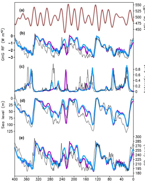
Figure 6. Transient simulations of the last four glacial cycles forced by orbital variations only (fully interactive experiments).
(a)Maximum summer insolation at 65◦N (W m−2);(b)radiative forcing (relative to pre-industrial) of well-mixed GHGs (W m−2);
(c) Antarctic dust deposition rate in relative units;(d)global ice volume expressed in sea level equivalent (m);(e)atmospheric CO2
concentration, ppm. Black line in(b)is radiative forcing of GHGs from Ganopolski and Calov (2011). Black dashed line in (c) is Antarctic dust from Augustin et al. (2004), in(d)is sea level stack from Spratt and Lisiecki (2016), and in(e)is compiled Antarctic CO2record from Lüthi et al. (2008). Blue lines in(d, e)correspond
to the fully interactive experiment INTER_1.0 and purple lines to the experiment INTER_1.1, where meltwater flux into the Atlantic was scaled up by a factor of 1.1.
and the first 150 kyr of the INTER_1.0 and ONE_1.0 experi-ments are in very good agreement, while during the time in-terval between 300 and 150 ka discrepancies are larger. This period corresponds to higher eccentricity and therefore to the larger magnitude of orbital forcing. Similarly to the results of one-way coupled experiments, the fully interactive exper-iments also show strong sensitivity to magnitude of freshwa-ter flux during glacial freshwa-terminations.
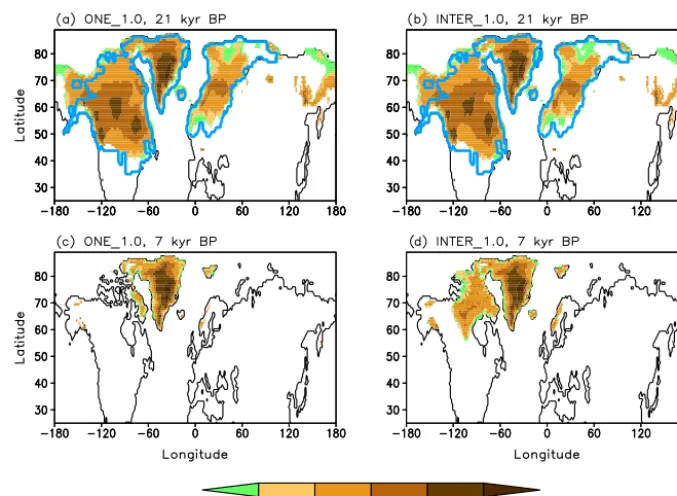
Comparison of simulated ice sheet spatial distribution and elevation (Fig. 7) shows that the results of one-way coupled (ONE_1.0, Fig. 6a) and the fully interactive experiments (IN-TER_1.0, Fig. 7b) are almost identical during the LGM (the same is true for the previous glacial maxima, not shown) and in reasonable agreement with the reconstructions.
Dur-ing glacial terminations, the difference between two experi-ments increases since in the fully interactive experiment the radiative forcing of GHGs lags considerably behind the re-constructed one used in the one-way coupled experiment. As a result, at 7 ka continental ice sheets melted completely in the one-way coupled experiment (Fig. 7c) while in the fully interactive experiment, a relatively large ice sheet is still present in northeastern Canada (Fig. 7d).
It is instructive to compare frequency spectra of simu-lated and reconstructed global ice volume in the one-way and fully interactive experiments (Fig. 8). In addition, Fig. 8 shows results from the experiment ONE_240 performed with constant radiative forcing of GHGs corresponding to equiv-alent CO2concentration of 240 ppm. As already shown by Ganopolski and Calov (2011), even with constant CO2, the model computes pronounced glacial cycle with 100 kyr peri-odicity, although it has much weaker amplitude than the re-constructed ice volume. Both model experiments with vary-ing CO2radiative forcing (ONE_1.0 and INTER_1.0) reveal much stronger 100 kyr periodicity, which has only a slightly weaker amplitude than the spectrum of the reconstructed ice volume. Interestingly, frequency spectra of ice volume sim-ulated in the one-way and fully interactive experiments have similar powers in 100 kyr and obliquity (40 kyr) bands, but in the precessional band (ca. 20 kyr) the one-way coupled experiment reveals a much higher spectral power. This can-not be explained by the prescribed radiative forcing of GHGs because the latter contain very little precessional variability. The stronger precessional component in the ONE_1.0 exper-iment is explained by the fact that in the one-way coupled experiment, the model simulates faster ice sheet growth dur-ing the initial part of each glacial cycle and the modelled ice volume variability at the precessional frequency is very sen-sitive to the global ice volume.
4 The composition of “the carbon stew” and factor analysis
suc-Figure 7.Simulated ice sheet elevation (m) at 21 ka(a, b)and 7 ka(c, d)in the one-way coupled experiment ONE_1.0(a, c)and fully interactive experiment INTER_1.0(b, d). Blue lines represent Ice-5g reconstruction at the LGM (Peltier, 2004).
cessful simulations of glacial cycles. The aim of our paper is not to present the ultimate solution for the “carbon stew” problem since at present this is impossible. Rather we want to demonstrate that with a reasonable representation of phys-ical, geochemphys-ical, and biological processes in the model, it is possible to reproduce the main features of Earth system dynamics over the past 400 kyr, including the magnitude and timing of climate, ice volume, and CO2variations.
Similar to the study by Brovkin et al. (2012), we per-formed a set of experiments using the one-way coupling tech-nique (see Table 1 for details). We use this approach instead of fully interactive coupling to exclude complex and strongly nonlinear interactions associated with the ice sheet dynam-ics, which significantly complicates the factor analysis. In the case of the one-way coupled experiments, climate, ice sheets, and other external factors are identical, and these ex-periments only differ from each other by the parameters of the carbon cycle model. Since CO2 simulated in the one-way coupled experiment with 10 % enhanced meltwater flux (ONE_1.1) is in a slightly better agreement with observa-tional data than the standard one (ONE_1.0), for the factor analysis we used the experiment ONE_1.1 as the reference one and performed all sensitivity experiments with 10 % en-hanced meltwater flux.
4.1 The standard carbon cycle model setup
We begin our analysis with the experiment that incorpo-rates only the standard ocean biogeochemistry as described
in Brovkin et al. (2007) (Fig. 9). This experiment does not in-clude the effect of the terrestrial carbon cycle. In this configu-ration, the model is able to explain only about 45 ppm of CO2 reduction during glacial cycles. Note that this experiment ac-counts for glacial–interglacial changes in ocean volume of ca. 3 % and corresponding changes in the total biogeochem-ical inventories including salinity. These volume changes are often neglected in simulations with 3-dimensional ocean models (e.g. Heinze et al., 2016), although these changes have substantial impact on the global carbon cycle, and in our simulations they counteract glacial CO2 drawdown by ca. 12 ppm. Without the effect of ocean volume reduction, the combination of physical processes and carbonate chemistry can explain up to 57 ppm at the LGM and on average 38 ppm during the entire 400 kyr time interval (see Table 2). This is consistent with the recent results by Buchanan et al. (2016) and Kobayashi et al. (2015). Note that simulated changes in silicate weathering and its impact on atmospheric CO2 are small, as has already been shown in Brovkin et al. (2012).
(a)
(b)
(c) (d)
Figure 8.Transient simulations of the last four glacial cycles forced by orbital variations, with prescribed, interactive, and fixed concen-trations of well-mixed GHGs.(a)Maximum summer insolation at 65◦N (W m−2);(b)temporal evolution of reconstructed and simu-lated sea level (m);(c)frequency spectra of the global ice volume;
(d) frequency spectra of boreal summer insolation. Black line is for the data (Spratt and Lisiecki, 2016), blue line corresponds to the one-way coupled experiment ONE_1.0, red line to the fully in-teractive experiment INTER_1.0, and green line to the ONE_240 experiment with constant (240 ppm) CO2concentration.
With all these processes considered in our previous study (Brovkin et al., 2012), we are still short of ca. 25 ppm to ex-plain the full magnitude of glacial–interglacial variability.
4.2 Additional processes included in the carbon cycle model
There are a number of other proposed mechanisms which potentially can explain several tens of ppm of glacial CO2 decline. Our choice of two processes to obtain the observed magnitude of glacial–interglacial CO2 variations is some-what subjective. The chosen mechanisms are explained be-low, while an alternative one (brine rejection) is discussed in Sect. 4.3.
The first additional mechanism added to the mech-anisms already described in Brovkin et al. (2012) is temperature-dependent remineralisation depth. In the stan-dard CLIMBER-2 version, remineralisation depth is spatially and temporally constant. Since in the colder ocean reminer-alisation depth increases, this enhances the efficiency of the carbon pump and contributes to a decrease in atmospheric CO2concentration (e.g. Heinze et al., 2016; Menviel et al., 2012; Matsumoto, 2007). Details of the mechanism imple-mentation are described in the Appendix. As seen in Fig. 9e,
(a)
(b)
(c)
(d)
(e)
Figure 9. Results of factor separation analysis. (a) Simulated CO2 (ppm) in one-way coupled ONE_1.1 experiment (purple line) and reconstructed CO2 concentrations (black dashed line,
Lüthi et al., 2008).(b)–(d)Contributions to simulated atmospheric CO2 (ppm) of terrestrial carbon cycle (b), ONE_S4–ONE_S3;
iron fertilisation (c), ONE_S3–ONE_S2; variable volcanic out-gassing(d), ONE_S2–ONE_S1; temperature-dependent remineral-isation depth(e), ONE_S1–ONE_1.1.
making remineralisation depth temperature dependent intro-duces additional glacial–interglacial variability of CO2with a magnitude of about 20 ppm. Roughly half of this value is clearly attributed to the CO2 overshoots seen at the begin-ning of some interglacials. The reason is that the AMOC shutdowns due to meltwater flux that happened during glacial terminations lead not only to surface cooling in the North At-lantic but also to significant thermocline warming that occurs over the entire Atlantic Ocean (e.g. Mignot et al., 2007). This subsurface warming causes pronounced shoaling of the rem-ineralisation depth and the release of carbon from the ocean into the atmosphere. This process reverses after recovery of the AMOC at the beginning of interglacials.
out-Table 1.Model experiments performed in this study. P denotes prescribed characteristic; I – interactive; STD – standard model configuration; RD – variable remineralisation depth; VO – variable volcanic outgassing; IF – iron fertilisation in the Southern Ocean; TC – terrestrial carbon cycle; BR – brine rejection mechanism. A minus sign means that the process is excluded and a plus sign means that process is included. Ice sheets are interactive in all simulations.
Experiment Radiative Southern Atlantic Model forcing of Ocean freshwater configuration GHGs dust factor
400 000-year experiments
ONE_1.0 P P 1 STD
ONE_1.1 P P 1.1 STD
ONE_S1 P P 1.1 STD−RD ONE_S2 P P 1.1 STD−RD−VO ONE_S3 P P 1.1 STD−RD−VO−IF ONE_S4 P P 1.1 STD−RD−VO−IF−TC ONE_240 240 ppm P 1 STD
INTER_1.0 I I 1 STD
INTER_1.1 I I 1.1 STD 130 000-year experiments
ONE_1.0_130K P P 1 STD ONE_1.1__130K P P 1.1 STD ONE_BRINE_130K P P 1 STD+BR
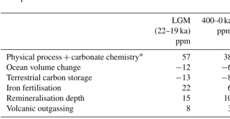
Table 2.“The carbon stew” at the LGM and the entire 400 kyr pe-riod in the ONE_1.1 experiment. Positive (negative) sign indicates that the process contributes to glacial CO2reduction (increase) as
compared to the pre-industrial concentration simulated at the end of the experiment.
LGM 400–0 ka (22–19 ka) ppm
ppm
Physical process+carbonate chemistry∗ 57 38
Ocean volume change −12 −6
Terrestrial carbon storage −13 −8
Iron fertilisation 22 6
Remineralisation depth 15 10
Volcanic outgassing 8 3
Total 77 43
∗
Deep ocean and shallow water carbonate sediments, carbonate and silicate weathering.
gassing and temperature-dependent remineralisation depth, CLIMBER-2 reproduces glacial–interglacial CO2cycles in a good agreement with paleoclimate records (Fig. 9a).
4.3 Brine rejection mechanism
Using a different version of CLIMBER-2, Bouttes et al. (2010) proposed that a significant fraction of glacial– interglacial CO2 variations can be explained by the mech-anism of brine rejections – more specifically, by a large increase in the depth to which brines can penetrate under glacial conditions without significant mixing with ambient
ef-ficiency. Mariotti et al. (2016) assumed an abrupt decrease in brine rejection efficiency from 0.7 to 0 in a very short interval between 18 and 16 ka. However, both sea level and the size of the Antarctic ice sheets remained essentially constant during this period and therefore there is no obvious reason for such large variations in the brine rejection efficiency. According to the interpretation of Roberts et al. (2016), brine rejection remained efficient during most of the glacial termination and ceased only after 11 ka, when most of the glacial–interglacial CO2rise had already been accomplished. In the view of these uncertainties, we decided not to include parameterisations of the brine rejection mechanism in simulations of glacial cy-cles. However, for simulations of the last glacial termination discussed below, we analysed the potential effect of brine re-jection on radiocarbon and other paleoclimate proxies.
5 Simulations of Termination I
5.1 Simulation of climate, CO2, and carbon isotopes
during the last termination
The last glacial termination provides a wealth of paleocli-mate records with a potential to better constrain the mecha-nisms of glacial CO2variability. In this section, we discuss the last glacial termination in more detail. Similarly to the previous section, to exclude nonlinear interaction with ice sheets, we discuss here only one-way coupled experiments. To reduce computational time, we performed experiments only for the last 130 000 years starting from the Eemian in-terglacial and using the same initial conditions as in the ex-periments discussed above.
In the standard ONE_1.0_130K experiment, the model simulates climate variability across Termination I rather real-istically. In particular, it reproduces the temporal resumption of the AMOC in the middle of the termination resembling the Bølling–Allerød warm event (Fig. 10a). However, the tim-ing of this event in our model is shifted by ca. 1000 years compared to the paleoclimate records. Results of our exper-iments reveal high sensitivity of the timing of the AMOC resumption to the magnitude of freshwater flux. A change of the flux by 10 % in the ONE_1.1_130K experiment sig-nificantly alters millennial-scale variability during the last glacial termination (Fig. 10). This result suggests that sim-ulated millennial-scale variability during the Termination I is not robust – i.e. it is unlikely that a single model run through the glacial termination would reproduce the right timing or even the right sequence of millennial-scale events.
Although simulated CO2 concentration at the LGM and pre-industrial state are close to observations, simulated CO2 appreciably lags behind reconstructed CO2during the termi-nation (Fig. 10b). This is primarily related to the fact that simulated CO2does not start to grow at ca. 18 ka BP as re-constructed, but only after the end of the simulated analogue of the Bølling–Allerød event. At the same time, in agree-ment with paleoclimate reconstructions, CO2 concentration
(a)
(b)
(c)
(d)
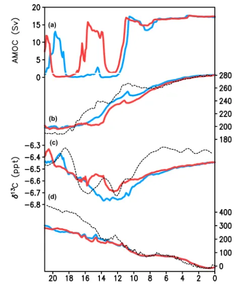
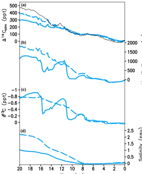
Figure 10.Simulation of Termination I with the set of one-way coupled models, which differ only in the scaling of freshwater flux. Blue line corresponds to the ONE_1.1_130K experiment with scal-ing factor 1.1, red line to the ONE_1.0_130K experiment with scaling factor 1.0.(a)AMOC strength (Sv);(b)atmospheric CO2
(ppm); (c) atmospheric δ13CO2 (‰); (d) atmospheric 114CO2 (‰). Dashed lines:(b, c)ice core data (Lüthi et al., 2008; Schmitt et al., 2012);(d)IntCal13 radiocarbon calibration curve (Reimer et al., 2013).
reaches a local maximum at the end of the North Atlantic cold event, which resembles the Younger Dryas event. Sim-ulated CO2concentration also reveals a continuous CO2rise during the Holocene towards its pre-industrial value of 280 ppm. This result confirms that such CO2dynamics could be explained by natural mechanisms alone and do not require early anthropogenic CO2emissions until ca. 2 ka (Kleinen et al., 2016). This result also demonstrates that the temporal dy-namics of CO2during interglacials critically depend on the timing of final AMOC recovery. Late recovery during glacial termination causes a strong overshoot of CO2at the begin-ning of the interglacial followed by some decrease or a stable CO2concentration. However, if the complete AMOC recov-ery occurs well before the end of termination, only temporal CO2overshoot occurs and CO2continues to rise during the entire interglacial.
(a) (b)
(c) (d)
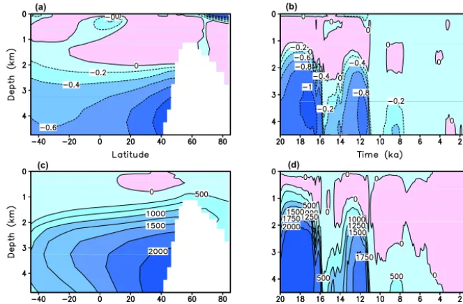
Figure 11.δ13C and radiocarbon ventilation age distribution in the Atlantic Ocean in the ONE_1.0_130K simulation of Termination I.
(a, b)δ13C (‰),(c, d)radiocarbon ventilation age in yr14C.(a, c)Differences between LGM (21 ka) and pre-industrial in the Atlantic Ocean.(b, d)Temporal evolution of anomalies during the past 20 kyr at 20◦N in the Atlantic.
Simulated atmospheric δ13C drops from the LGM level of about −6.4 ‰ to the minimum value of −6.7 ‰ between 16 and 14 ka (Fig. 10c). This is primarily related to the re-duction of marine biological productivity which, in turn, is explained by the decrease in iron fertilisation effect over the Southern Ocean during the first part of Termination I. The magnitude of theδ13C drop is in a good agreement with em-pirical data (Fig. 10c). The model is also able to simulate W-shapedδ13C evolution associated with reorganisation of the AMOC. However, this W shape is shifted in time com-pared to the reconstructed one by ca. 1000 years because the model analogue of the Bølling–Allerød event occurs ear-lier than the real one by the same amount of time. Note that this local maximum inδ13C is completely absent in the ex-periment ONE_1.1_130K, where temporal resumption of the AMOC during glacial termination does not occur.δ13C rise after 12 ka is primary attributed to the accumulation of car-bon in terrestrial carcar-bon pools (forest regrowth and peat ac-cumulation). At the same time, simulated present-day atmo-sphericδ13C is underestimated compared to ice core data by ca. 0.15 ‰.
The model simulates an almost monotonic decrease in at-mospheric 114C from the LGM to present. Most of this decrease (ca. 200 ‰) is caused by a prescribed production rate which was about 20 % higher during LGM. Only about 80 ‰ of114C is attributed to a difference in climate state be-tween LGM and the present, primarily due to a less ventilated deep ocean. As shown in Fig. 10d, simulated atmospheric 114C is significantly underestimated before 12 ka compared to the reconstruction by Reimer et al. (2013) and at the LGM
this difference reaches more than 100 ‰. It is possible but unlikely that such big differences can be attributed to uncer-tainties in reconstructed production rate. An alternative hy-pothesis for explaining this mismatch is discussed below.
Figure 11 shows LGM time slice anomalies and tempo-ral evolution ofδ13C and radiocarbon ventilation age during Termination I in the Atlantic Ocean simulated in experiment ONE_1.0_130K. The spatial distribution of glacial anoma-lies and temporal dynamics of δ13C and radiocarbon ven-tilation age during termination are qualitatively very simi-lar. Glacialδ13C in the deep Atlantic at the LGM is 0.6– 1 ‰ lower than at present; this is primarily related to a shoal-ing of the AMOC and reduced ventilation in the South-ern Ocean. The vertical distribution of δ13C anomalies at the LGM is consistent with the paleoclimate reconstructions (e.g. Hesse et al., 2011).
(a)
(b)
(c)
(d)
Figure 12. Simulation of Termination I in the stan-dard ONE_1.0_130K experiment (solid blue) and the ONE_BRINE_130K (dashed blue) experiment, which includes brine parameterisation and stratification-dependent vertical mixing.
(a)Atmospheric114C (in %◦).(b)Deep tropical Atlantic radio-carbon ventilation age (in yr14C).(c)Deep tropical Atlanticδ13C (%◦).(d)Deep Southern Ocean salinity (psu);(c, d)for the depth 4 km. Black dashed line is IntCal13 radiocarbon calibration curve (Reimer et al., 2013).
During glacial termination, both δ13C and radiocarbon ventilation age show pronounced response at all depths to the millennial-scale reorganisations of the AMOC (Fig. 12b and d). The ventilation age in the deep Atlantic, which is about 2000 years prior to the model analogue of the warm Bølling–Allerød event, rapidly reaches nearly the modern level after the AMOC resumption and drops again to the glacial level during the model analogue of the cold Younger Dryas event. Such evolution of ventilation age in the North Atlantic is in agreement with paleoclimate reconstructions (Robinson et al., 2005; Skinner et al., 2014).
5.2 Brine rejection mechanisms and radiocarbon in the ocean and atmosphere
As discussed above, our version of the CLIMBER-2 model is not able to accurately reproduce atmospheric14C decline during the first part of the last glacial termination. At the same time, Mariotti et al. (2016) demonstrated that their ver-sion of CLIMBER-2, which incorporates the mechanism of
(a) (b) (c)
Figure 13.Vertical profile of ventilation age in14C years for At-lantic(a), Pacific(b), and Southern Ocean(c). Red line represents modern conditions; solid blue – LGM in ONE_1.0_130K experi-ment using the standard version of the model; dashed blue – LGM in ONE_BRINE_130K experiment with the model version, which includes brine parameterisation and stratification-dependent verti-cal mixing. Red (blue) squares represent basin-averaged radiocar-bon age for the modern (LGM) state based on the data of Skinner et al. (2017).
Figure 14.Dynamics of terrestrial carbon pools (Gt C) in the one-way coupled ONE_1.0 simulation. Left panels: the whole 400 kyr period; right panels: the Termination I period.(a)Black line – total carbon storage; magenta line – conventional carbon pools (biomass and mineral soils).(b)–(d)Peat, permafrost, and buried carbon storages, respectively.
LGM, which is in good agreement with the 689±5314C yr reported in Skinner et al. (2017). At the same time, the model with the brine rejection parameterisation simulates an in-crease in the ventilation age of more than 130014C yr.
Interestingly, the two model versions do not differ much with respect to simulated deep oceanδ13C. Finally, the two model versions differ significantly with respect to the deep Southern Ocean salinity. Change in salinity in the standard model version is only about 1 psu, which is close to the global mean salinity change due to ice sheet growth. The model version with the brine rejection parameterisation sim-ulates glacial deep South Ocean salinity of 37 psu, which is in good agreement with the reconstruction by Adkins et al. (2002). Thus we found that including additional effects (brines and stratification-dependent diffusion) helps to bring atmospheric114C and the deep Southern Ocean salinity into better agreement with available reconstructions, but at the ex-pense of very old (likely to be at odds with paleoclimate data) water masses in the deep ocean. Of course, these results are obtained with a very simple ocean component and it is possi-ble that more realistic ocean models would be apossi-ble to resolve this apparent contradiction.
5.3 Changes in the terrestrial carbon cycle
The evolution of the carbon cycle in the one-way coupled simulation is presented in Fig. 13. The conventional com-ponents of the land carbon cycle (vegetation biomass, soil carbon stored in non-frozen and non-flooded environment)
change between 1400 Gt C during the LGM and 2000 Gt C during interglacial peaks. Such an amplitude of 600 Gt C of glacial–interglacial changes is typical for the models of the land carbon cycle without long-term components (Kaplan et al., 2002; Joos et al., 2004; Brovkin et al., 2002). How-ever, when we account for permafrost, peat, and buried car-bon, the magnitude decreases to 300–400 Gt C. This is due to the counteracting effect of the permafrost and buried carbon pools relative to the conventional components. Both these pools vary between 0 and 350 Gt C and reach their maxima during glacials. The peat storage also reaches about 350 Gt C, but it grows only during interglacials or warm stadials. Let us note that during glacial inceptions, while biomass and min-eral soil carbon decrease, terrestrial carbon storage increases due to an increase in buried and permafrost carbon. As a re-sult, total land carbon did not change much during the period of large ice sheet initiation.
6 Conclusions
We present here the first simulations of the last four glacial cycles with the one-way and two-way coupled carbon cycle model. The model is able to reproduce the major aspects of glacial–interglacial variability of climate, ice sheets, and of atmospheric CO2concentration even when driven by the or-bital forcing alone. These results provide strong support to the idea that long and strongly asymmetric glacial cycles of the late Quaternary represent a direct but strongly nonlinear response of the Northern Hemisphere ice sheets to the orbital forcing which, in turn, is amplified and globalised by the car-bon cycle feedback.
The model simulates correct timing of the past glacial ter-minations in terms of ice volume while the simulated CO2 concentration lags behind the reconstructed one by several thousand years. The model is also able to simulate tempo-ral evolution of the stable carbon isotope in the ocean. At the same time, the agreement between simulated and recon-structed atmosphericδ13C is rather poor. Similarly, the mag-nitude of simulated atmospheric14C decline during the last glacial termination is underestimated. Introducing the brine rejection parameterisation and stratification-dependent ver-tical diffusivity allows us to improve the agreement for at-mospheric14C but leads to unrealistically “old” glacial deep ocean water masses.
The temporal dynamics of CO2during interglacial depend strongly on the timing of the AMOC recovery during glacial termination. If the AMOC recovers only at the end of glacial termination, CO2concentration experiences an overshoot at the beginning of interglacial and then CO2declines. In con-trast, early recovery of the AMOC leads to a monotonic rise of CO2during interglacials. In our simulations, millennial-scale variability during the last glacial termination is very sensitive to the magnitude of meltwater flux, and the se-quence and timing of simulated millennial-scale events are not robust even when the model is forced by prescribed ra-diative forcing of GHGs.
Adding new long-term carbon pools (peat, buried and permafrost carbon) decreases the amplitude of glacial– interglacial changes in the total land carbon storage. It helps to reduce an effect of terrestrial biosphere on the CO2change during glacial inception and to a lesser extent during glacial terminations.
This work demonstrates that simulation of glacial cycles with Earth system models driven by orbital forcing alone is possible. This does not mean that we have presented here the ultimate recipes for all processes and feedbacks and, in particular, for “the carbon stew”. The understanding of how the global carbon cycle operates on orbital and suborbital timescales still remains incomplete, and large uncertainties remain in the choice of individual processes and their pa-rameterisations. Paleoclimate data provide some useful con-straints but the proxy data syntheses are far from being in a perfect state, with some proxies telling contradictory stories and others being difficult to interpret.
The CLIMBER-2 model is a rather simple and coarse res-olution Earth system model. This allows us to perform a large ensemble of model simulations on orbital and even longer timescales. Obviously, such a fast model has signif-icant limitations. In particular, it employs the zonally aver-aged ocean model. Many essential processes, such as iron fertilisation effect, are parameterised. The development of a high-resolution state-of-the-art Earth system model suitable for simulation of the interaction between climate, ice sheets, and carbon cycle at orbital timescales is crucial to make the next step forward in understanding of Earth system dynamics during the Quaternary.
Appendix A: Appendix A
A1 Modifications of terrestrial carbon cycle model The old version of the CLIMBER-2 carbon cycle model de-scribed in Brovkin et al. (2002) considers two vegetation types – trees and grass. Each of the two vegetation types has four carbon pools – leaves, stems, and fast and slow soil carbon. Each of these four pools occupies the same frac-tion of grid cell as the respective vegetafrac-tion type. Crichton et al. (2014) in their version of permafrost carbon implementa-tion in CLIMBER-2 have not changed the pool structure but modified turnover time, assuming that it is increasing under permafrost conditions. In the new version of the carbon cycle model which we use in the present work, we have introduced three new carbon pools: boreal peat, permafrost, and carbon buried under ice sheets. The fractions of land covered by grass and trees are computed in the vegetation model follow-ing Brovkin et al. (1997), the fraction of land covered by ice sheets is computed by the ice sheet model and the fraction of permafrostfpmfor the temperature range−5◦C< Tts<5◦C is computed in the land surface module as
fpm=0.5−0.1Tts,
where Tts is annual mean top soil layer temperature. It is assumed that grass (in boreal latitudes this mean tundra) is located north of forest and therefore freezes first. Only if permafrost exceeds grass fraction can the permafrost expand over the area covered with trees. During ice sheet growth, all carbon under ice sheets apart from the living biomass is re-allocated into the buried carbon pool. Buried carbon remains intact until it is covered by ice sheets. During deglaciation, this buried carbon is transformed into the permafrost pool. The fraction of land covered by peat is defined as
fpt=fpt∗ 1−fgc−fpm,
wherefpt∗ is the potential fraction of peat in each grid cell prescribed from modern observational data and fgc is the fraction of land covered by ice sheets. Note that we do not consider peatlands in low latitudes. Although peat and per-mafrost have certain areal fractions, they are considered to be parts of grid cells covered by vegetation. Net primary produc-tion and fluxes between the fast carbon pools (leaves, stems, and fast soil pool) are computed the same way as in Brovkin et al. (2012). The downward flux of carbon from the fast soil is partitioned between slow soil pool and permafrost propor-tionally to their relative fractions. The rate of peat accumu-lation is equal to a fixed fraction of net primary production in the respective vegetation type. Evolution of carbon con-tentpi in slow carbon pools is described by the equation
dpi
dt =qifi+ dfi
dt b
0 i,
wherepi=bifi, thebi is the concentration of carbon in the
ith carbon pool (in kgC m−2), andfi is the fraction of the
ith pool. The valueqi represents the difference between local
accumulation and decay of carbon in the pool,b0i is carbon concentration in the pool by which theith pool is expanded, andb0i=bi if theith pool is shrinking. For peat,bi0=0. For
the permafrost, the situation is more complex, because it can gain/lose carbon from/to slow soil, peat, and buried carbon pools. The source term for the permafrost poolqpmconsists
of the sum of fluxes from the fast grassland and tree soil pools into the respective slow pools (see Brovkin et al., 2002, for details) minus the decay term, where the decay timescale is set to 20 000 years. Apart from carbon, the terrestrial carbon model also computes carbon isotope (13C and14C) contents in all carbon pools. Since carbon isotopes are also computed in the oceanic carbon cycle model, we can computeδ13C and δ14C in the atmosphere and compare modelling results with available paleoclimate data.
A2 Modifications of the ocean carbon cycle model A2.1 Dust deposition in the Southern Ocean
In the one-way coupled experiments, similar to Brovkin et al. (2012), we used the concentration of aeolian dust in the Antarctic ice cores as the proxy for iron deposition over the Southern Ocean. Such choice is supported by the recent mea-surements of iron content in Southern Ocean sediment cores (Lamy et al., 2014). In the fully interactive run, the iron flux over the Southern Ocean (D) in arbitrary units is parame-terised through the global sea level change as
D=
100dS dt +10
max(S−50;0)+1.5S,
whereS is the ice volume expressed in metres of sea level equivalent and timet is in years. This formula gives signif-icant increase in iron flux for the case when sea level drops below 50 m, which is likely related to the fact that Patago-nian dust source is very sensitive to the area of exposed shelf and glacial erosion processes. Numerical parameters in this formula were obtained by fitting simulatedD to dust con-centration in the Antarctic record. This allows us to use the same parameterisation for the iron fertilisation effect in the one-way and fully interactive experiments. To prevent large fluctuations in the iron flux related to fluctuations of the time derivative ofS, the dust depositionDcomputed by this equa-tion has been smoothed by applying a relaxaequa-tion procedure. Namely, at each time stepn, the dust depositionDnis
com-puted as
Dn=(1−ε)D+εDn−1,
A2.2 Dependence of remineralisation depth on temperature
In CLIMBER-2 the vertical profile of carbon below the eu-photic zone is given by
f(z)=
z
zr −0.858
,
where remineralisation depth zr is held constant equal to
100 m. To take into account the dependence of reminerali-sation rate on ambient temperature, following Segschneider and Bendtsen (2013), we now use the dependence of zr on the thermocline temperature (300 m)T:
zr=zro2−
T−T0 10 ,
where T0=9◦C and zro=100 m. The value of T0 was selected in such a way that introducing the temperature-dependent remineralisation depth does not affect atmo-spheric CO2concentration under pre-industrial climate con-ditions. During glacial times, temperature in the thermo-cline decreases by 2–3◦C, which causes an increase in zr by 20–30 %. This results in additional CO2 drawdown by ca. 15 ppm.
A2.3 Parameterisation of the iron fertilisation effect The rate of dust deposition which is prescribed from the ice cores in the one-way coupled experiment or computed from global ice volume in the fully interactive experiments is con-sidered to be a proxy for iron flux and is used in the eterisation of iron the fertilisation mechanism. This param-eterisation is only applied to the Southern Ocean (south of 40◦S). As described in Brovkin et al. (2002), net primary production of phytoplankton5in the model is computed as
5=c(D)r(T , R) P P+P0
Cp(1−f), (A1)
whereCpis the phytoplankton concentration,P is the phos-phorus concentration in the euphotic zone,ris a function of temperature T and photosynthetic active insolationR,f is the fraction of grid cell covered by sea ice,P0is a constant, andcis a function of normalised dust deposition rateD. Note that in the case of prescribed dust deposition rate,Dwas ob-tained by multiplying observed dust concentration in mg g−1 units by factor 10−3. North of 40◦S, parametercis set to 1 and south of 40◦S
c=min (1,0.1+cdD),
wherecd=2. During glacial maxima the value ofcreaches a value of about 1, which implies that during these periods there is no iron limitation in the Southern Ocean. During interglacials, when D is much smaller than 100, cis close to 0.1. The parameters of this parameterisation have been se-lected (i) to reproduce present-day nutrient concentration in
the Southern Ocean, and (ii) to obtain 20–30 ppm additional CO2drawdown during glacial maxima due to the iron fertil-isation effect.
A3 Variable volcanic outgassing
Following the idea of Huybers and Langmuir (2009), which has been tested already in Roth and Joos (2012), we intro-duced a dependence of volcanic CO2 outgassingO on the rate of sea level change. Namely, we assume that volcanic outgassing linearly depends on sea level derivative with the time delay of about 5000 years:
O(t)=O1
1−O2
dS(t−5000) dt
.
HereO1=5.3 Tmol C yr−1 andO2=50 Tmol C m−1. With these parameters, volcanic outgassing does not change by more than 30 % during all glacial cycles. Note that over one glacial cycle the average value ofOis very close toO1.
A4 Calculation of radiocarbon ventilation age
For the direct comparison of model results with the empiri-cal reconstruction of marine radiocarbon age offset (Skinner et al., 2017), we calculate the model analogue of this charac-teristic using simulated relative concentration of the radiocar-bon in the atmospherecatm=14Catm/12Catmand in the ocean cocn=14Cocn/12Cocnusing the formula
t= −8033 ln
c ocn
catm
.
A5 Modifications of the energy and surface mass balance interface
Competing interests. The authors declare that they have no con-flict of interest.
Acknowledgements. The authors thank Edouard Bard and Fortunat Joos for helpful discussion of the atmospheric and oceanic 14C dynamics and Luke Skinner for useful comments and suggestions. The authors acknowledge support of the German Ministry of Education and Research (PalMod project).
Edited by: André Paul
Reviewed by: Luke Skinner and one anonymous referee
References
Abe-Ouchi, A., Saito, F., Kawamura, K., Raymo, M. E., Okuno, J., Takahashi, K., and Blatter, H.: Insolation-driven 100,000-year glacial cycles and hysteresis of ice-sheet volume, Nature, 500, 190–194, https://doi.org/10.1038/nature12374, 2013.
Adkins, J. F., McIntyre, K., and Schrag, D. P.: The salinity, temper-ature, andδ18O of the glacial deep ocean, Science, 298, 1769– 1773, https://doi.org/10.1126/science.1076252, 2002.
Archer, D.: A data-driven model of the global cal-cite lysocline, Global Biogeochem. Cy., 10, 511–526, https://doi.org/10.1029/96gb01521, 1996.
Archer, D., Winguth, A., Lea, D., and Mahowald, N.: What caused the glacial/interglacial atmosphericpCO2cycles?, Rev.
Geophys., 38, 159–189, https://doi.org/10.1029/1999rg000066, 2000.
Arz, H. W., Lamy, F., Ganopolski, A., Nowaczyk, N., and Patzold, J.: Dominant Northern Hemisphere climate control over millennial-scale glacial sea-level variability, Quaternary Sci. Rev., 26, 312–321, https://doi.org/10.1016/j.quascirev.2006.07.016, 2007.
Augustin, L., Barbante, C., Barnes, P. R. F., Barnola, J. M., Bigler, M., Castellano, E., Cattani, O., Chappellaz, J., DahlJensen, D., Delmonte, B., Dreyfus, G., Durand, G., Falourd, S., Fischer, H., Fluckiger, J., Hansson, M. E., Huybrechts, P., Jugie, R., Johnsen, S. J., Jouzel, J., Kaufmann, P., Kipfstuhl, J., Lam-bert, F., Lipenkov, V. Y., Littot, G. V. C., Longinelli, A., Lor-rain, R., Maggi, V., Masson-Delmotte, V., Miller, H., Mul-vaney, R., Oerlemans, J., Oerter, H., Orombelli, G., Parrenin, F., Peel, D. A., Petit, J. R., Raynaud, D., Ritz, C., Ruth, U., Schwander, J., Siegenthaler, U., Souchez, R., Stauffer, B., Stef-fensen, J. P., Stenni, B., Stocker, T. F., Tabacco, I. E., Udisti, R., van de Wal, R. S. W., van den Broeke, M., Weiss, J., Wil-helms, F., Winther, J. G., Wolff, E. W., and Zucchelli, M.: Eight glacial cycles from an Antarctic ice core, Nature, 429, 623–628, https://doi.org/10.1038/nature02599, 2004.
Barnola, J. M., Raynaud, D., Korotkevich, Y. S., and Lorius, C.: Vostok ice core privides 160,000-year record of atmospheric CO2, Nature, 329, 408–414, https://doi.org/10.1038/329408a0,
1987.
Berger, A., Li, X. S., and Loutre, M. F.: Modelling northern hemi-sphere ice volume over the last 3 Ma, Quaternary Sci. Rev., 18, 1–11, https://doi.org/10.1016/s0277-3791(98)00033-x, 1999.
Bouttes, N., Paillard, D., and Roche, D. M.: Impact of brine-induced stratification on the glacial carbon cycle, Clim. Past., 6, 575–589, https://doi.org/10.5194/cp-6-575-2010, 2010.
Brady, E. C., Otto-Bliesner, B. L., Kay, J. E., and Rosenbloom, N.: Sensitivity to Glacial Forcing in the CCSM4, J. Climate, 26, 1901–1925, https://doi.org/10.1175/jcli-d-11-00416.1, 2013. Brovkin, V., Ganopolski, A., and Svirezhev, Y.: A
con-tinuous climate–vegetation classification for use in climate-biosphere studies, Ecol. Model., 101, 251–261, https://doi.org/10.1016/s0304-3800(97)00049-5, 1997.
Brovkin, V., Bendtsen, J., Claussen, M., Ganopolski, A., Ku-batzki, C., Petoukhov, V., and Andreev, A.: Carbon cycle, veg-etation, and climate dynamics in the Holocene: Experiments with the CLIMBER-2 model, Global Biogeochem. Cy., 16, 1139, https://doi.org/10.1029/2001gb001662, 2002.
Brovkin, V., Ganopolski, A., Archer, D., and Rahmstorf, S.: Lower-ing of glacial atmospheric CO2in response to changes in oceanic
circulation and marine biogeochemistry, Paleoceanography, 22, PA4202, https://doi.org/10.1029/2006pa001380, 2007.
Brovkin, V., Ganopolski, A., Archer, D., and Munhoven, G.: Glacial CO2cycle as a succession of key physical and biogeochemical
processes, Clim. Past., 8, 251–264, https://doi.org/10.5194/cp-8-251-2012, 2012.
Brovkin, V., Bruecher, T., Kleinen, T., Zaehle, S., Joos, F., Roth, R., Spahni, R., Schmitt, J., Fischer, H., Leuenberger, M., Stone, E. J., Ridgwell, A., Chappellaz, J., Kehrwald, N., Barbante, C., Blunier, T., and Jensen, D. D.: Comparative carbon cycle dynam-ics of the present and last interglacial, Quaternary Sci. Rev., 137, 15–32, https://doi.org/10.1016/j.quascirev.2016.01.028, 2016. Buchanan, P. J., Matear, R. J., Lenton, A., Phipps, S. J., Chase,
Z., and Etheridge, D. M.: The simulated climate of the Last Glacial Maximum and insights into the global marine carbon cy-cle, Clim. Past., 12, 2271–2295, https://doi.org/10.5194/cp-12-2271-2016, 2016.
Burley, J. M. A. and Katz, R. F.: Variations in mid-ocean ridge CO2 emissions driven by glacial cycles, Earth Planet. Sc. Lett., 426, 246–258, https://doi.org/10.1016/j.epsl.2015.06.031, 2015. Calov, R., Ganopolski, A., Claussen, M., Petoukhov, V., and Greve,
R.: Transient simulation of the last glacial inception. Part I: glacial inception as a bifurcation in the climate system, Clim. Dy-nam., 24, 545–561, https://doi.org/10.1007/s00382-005-0007-6, 2005.
Ciais, P., Tagliabue, A., Cuntz, M., Bopp, L., Scholze, M., Hoff-mann, G., Lourantou, A., Harrison, S. P., Prentice, I. C., Kel-ley, D. I., Koven, C., and Piao, S. L.: Large inert carbon pool in the terrestrial biosphere during the Last Glacial Maximum, Nat. Geosci., 5, 74–79, https://doi.org/10.1038/ngeo1324, 2012. Crichton, K. A., Bouttes, N., Roche, D. M., Chappellaz, J., and
Krinner, G.: Permafrost carbon as a missing link to explain CO2
changes during the last deglaciation, Nat. Geosci., 9, 683–686, https://doi.org/10.1038/ngeo2793, 2014.
Crowley, T. J. and Hyde, W. T.: Transient nature of late Pleistocene climate variability, Nature, 456, 226–230, https://doi.org/10.1038/nature07365, 2008.
Eggleston, S., Schmitt, J., Bereiter, B., Schneider, R., and Fischer, H.: Evolution of the stable carbon isotope composition of atmo-spheric CO2over the last glacial cycle, Paleoceanography, 31,
Fischer, H., Schmitt, J., Luthi, D., Stocker, T. F., Tschumi, T., Parekh, P., Joos, F., Köhler, P., Volker, C., Gersonde, R., Bar-bante, C., Le Floch, M., Raynaud, D., and Wolff, E.: The role of Southern Ocean processes in orbital and millennial CO2
variations – A synthesis, Quaternary Sci. Rev., 29, 193–205, https://doi.org/10.1016/j.quascirev.2009.06.007, 2010.
Galbraith, E. D. and Jaccard, S. L.: Deglacial weakening of the oceanic soft tissue pump: global constraints from sedimentary nitrogen isotopes and oxygenation proxies, Quaternary Sci. Rev., 109, 38–48, https://doi.org/10.1016/j.quascirev.2014.11.012, 2015.
Ganopolski, A. and Brovkin, V.: The last four glacial CO2cycles simulated with the CLIMBER-2 model, in: Deglacial Changes in Ocean Dynamics and Atmospheric CO2. Modern, Glacial,
and Deglacial Carbon Transfer between Ocean, Atmosphere, and Land, edited by: Sarnthein, M. and Haug, G., Deutsche Akademie der Naturforscher Leopoldina, Halle (Saale), 75–80, 2015.
Ganopolski, A. and Calov, R.: The role of orbital forcing, carbon dioxide and regolith in 100 kyr glacial cycles, Clim. Past., 7, 1415–1425, https://doi.org/10.5194/cp-7-1415-2011, 2011. Ganopolski, A. and Roche, D. M.: On the nature of
lead-lag relationships during glacial-interglacial cli-mate transitions, Quaternary Sci. Rev., 28, 3361–3378, https://doi.org/10.1016/j.quascirev.2009.09.019, 2009.
Ganopolski, A., Petoukhov, V., Rahmstorf, S., Brovkin, V., Claussen, M., Eliseev, A., and Kubatzki, C.: CLIMBER-2: a climate system model of intermediate complexity. Part II: model sensitivity, Clim. Dynam., 17, 735–751, https://doi.org/10.1007/s003820000144, 2001.
Ganopolski, A., Calov, R., and Claussen, M.: Simulation of the last glacial cycle with a coupled climate ice-sheet model of intermediate complexity, Clim. Past, 6, 229–244, https://doi.org/10.5194/cp-6-229-2010, 2010.
Ganopolski, A., Winkelmann, R., and Schellnhuber, H. J.: Critical insolation-CO2 relation for diagnosing past
and future glacial inception, Nature, 529, 200–204, https://doi.org/10.1038/nature16494, 2016.
Greve, R.: A continuum-mechanical formulation for shallow poly-thermal ice sheets, Philos. T. Roy. Soc. A, 355, 921–974, https://doi.org/10.1098/rsta.1997.0050, 1997.
Hain, M. P., Sigman, D. M., and Haug, G. H.: Distinct roles of the Southern Ocean and North Atlantic in the deglacial atmo-spheric radiocarbon decline, Earth Planet. Sc. Lett., 394, 198– 208, https://doi.org/10.1016/j.epsl.2014.03.020, 2014.
Heinze, C., Hoogakker, B. A. A., and Winguth, A.: Ocean car-bon cycling during the past 130 000 years – a pilot study on inverse palaeoclimate record modelling, Clim. Past., 12, 1949– 1978, https://doi.org/10.5194/cp-12-1949-2016, 2016.
Hesse, T., Butzin, M., Bickert, T., and Lohmann, G.: A model-data comparison ofδ13C in the glacial Atlantic Ocean, Paleoceanog-raphy, 26, PA3220, https://doi.org/10.1029/2010PA002085, 2011.
Huybers, P. and Langmuir, C.: Feedback between deglaciation, vol-canism, and atmospheric CO2, Earth Planet. Sci. Lett., 286, 479–
491, https://doi.org/10.1016/j.epsl.2009.07.014, 2009.
Jaccard, S. L., Galbraith, E. D., Martinez-Garcia, A., and Anderson, R. F.: Covariation of deep Southern Ocean oxygenation and
at-mospheric CO2through the last ice age, Nature, 530, 207–210,
https://doi.org/10.1038/nature16514, 2016.
Joos, F., Gerber, S., Prentice, I. C., Otto-Bliesner, B. L., and Valdes, P. J.: Transient simulations of Holocene atmo-spheric carbon dioxide and terrestrial carbon since the Last Glacial Maximum, Global Biogeochem. Cy., 18, GB2002, https://doi.org/10.1029/2003gb002156, 2004.
Jouzel, J., Masson-Delmotte, V., Cattani, O., Dreyfus, G., Falourd, S., Hoffmann, G., Minster, B., Nouet, J., Barnola, J. M., Chappellaz, J., Fischer, H., Gallet, J. C., Johnsen, S., Leuen-berger, M., Loulergue, L., Luethi, D., Oerter, H., Parrenin, F., Raisbeck, G., Raynaud, D., Schilt, A., Schwander, J., Selmo, E., Souchez, R., Spahni, R., Stauffer, B., Steffensen, J. P., Stenni, B., Stocker, T. F., Tison, J. L., Werner, M., and Wolff, E. W.: Orbital and millennial Antarctic climate vari-ability over the past 800,000 years, Science, 317, 793–796, https://doi.org/10.1126/science.1141038, 2007.
Kaplan, J. O., Prentice, I. C., Knorr, W., and Valdes, P. J.: Modeling the dynamics of terrestrial carbon storage since the Last Glacial Maximum, Geophys. Res. Lett., 29, 2074, https://doi.org/10.1029/2002gl015230, 2002.
Kleinen, T., Brovkin, V., and Munhoven, G.: Modelled interglacial carbon cycle dynamics during the Holocene, the Eemian and Marine Isotope Stage (MIS) 11, Clim. Past., 12, 2145–2160, https://doi.org/10.5194/cp-12-2145-2016, 2016.
Kleypas, J. A.: Modeled estimates of global reef habitat and car-bonate production since the last glacial maximum, Paleoceanog-raphy, 12, 533–545, https://doi.org/10.1029/97pa01134, 1997. Kobayashi, H., Abe-Ouchi, A., and Oka, A.: Role of
South-ern Ocean stratification in glacial atmospheric CO2
re-duction evaluated by a three-dimensional ocean general circulation model, Paleoceanography, 30, 1202–1216, https://doi.org/10.1002/2015pa002786, 2015.
Köhler, P., Fischer, H., and Schmitt, J.: Atmospheric δ13CO2
and its relation to pCO2 and deep ocean δ13C dur-ing the late Pleistocene, Paleoceanography, 25, PA1213, https://doi.org/10.1029/2008pa001703, 2010.
Kovaltsov, G. A., Mishev, A., and Usoskin, I. G.: A new model of cosmogenic production of radiocarbon 14C in the atmosphere, Earth Planet. Sc. Lett., 337, 114–120, https://doi.org/10.1016/j.epsl.2012.05.036, 2012.
Lambert, F., Tagliabue, A., Shaffer, G., Lamy, F., Winckler, G., Farias, L., Gallardo, L., and De Pol-Holz, R.: Dust fluxes and iron fertilization in Holocene and Last Glacial Maximum climates, Geophys. Res. Lett., 42, 6014–6023, https://doi.org/10.1002/2015gl064250, 2015.
Lamy, F., Gersonde, R., Winckler, G., Esper, O., Jaeschke, A., Kuhn, G., Ullermann, J., Martinez-Garcia, A., Lambert, F., and Kilian, R.: Increased Dust Deposition in the Pacific South-ern Ocean During Glacial Periods, Science, 343, 403–407, https://doi.org/10.1126/science.1245424, 2014.
Lisiecki, L. E., Raymo, M. E., and Curry, W. B.: Atlantic overturn-ing responses to Late Pleistocene climate forcoverturn-ings, Nature, 456, 85–88, https://doi.org/10.1038/nature07425, 2008.