© Author(s) 2009. This work is distributed under the Creative Commons Attribution 3.0 License.
of the Past
Changes in atmospheric variability in a glacial climate and the
impacts on proxy data: a model intercomparison
F. S. R. Pausata1,2, C. Li1,3, J. J. Wettstein1, K. H. Nisancioglu1, and D. S. Battisti4,2
1Bjerknes Centre for Climate Research, Allegaten 55, 5007 Bergen, Norway 2Geophysical Institute, University of Bergen, Allegaten 70, 5007 Bergen, Norway 3Department of Earth Science, University of Bergen, Allegaten 41, 5007 Bergen, Norway 4Department of Atmospheric Sciences, University of Washington, Seattle, WA 98195, USA
Received: 11 February 2009 – Published in Clim. Past Discuss.: 12 March 2009 Revised: 1 August 2009 – Accepted: 21 August 2009 – Published: 11 September 2009
Abstract. Using four different climate models, we investi-gate sea level pressure variability in the extratropical North Atlantic in the preindustrial climate (1750 AD) and at the Last Glacial Maximum (LGM, 21 kyrs before present) in or-der to unor-derstand how changes in atmospheric circulation can affect signals recorded in climate proxies.
In general, the models exhibit a significant reduction in interannual variance of sea level pressure at the LGM com-pared to pre-industrial simulations and this reduction is con-centrated in winter. For the preindustrial climate, all models feature a similar leading mode of sea level pressure variabil-ity that resembles the leading mode of variabilvariabil-ity in the in-strumental record: the North Atlantic Oscillation (NAO). In contrast, the leading mode of sea level pressure variability at the LGM is model dependent, but in each model differ-ent from that in the preindustrial climate. In each model, the leading (NAO-like) mode of variability explains a smaller fraction of the variance and also less absolute variance at the LGM than in the preindustrial climate.
The models show that the relationship between atmo-spheric variability and surface climate (temperature and pre-cipitation) variability change in different climates. Results are model-specific, but indicate that proxy signals at the LGM may be misinterpreted if changes in the spatial pattern and seasonality of surface climate variability are not taken into account.
Correspondence to: F. S. R. Pausata
1 Introduction
Much of our knowledge about past climates comes from only a few locations, most notably Greenland and Antarctica, be-cause it is difficult to obtain good quality, high resolution proxy records of long duration. It follows that data from sin-gle locations have been used to infer climate changes back in time at regional, hemispheric and even global spatial scales (e.g. Dansgaard et al., 1993; Jouzel et al., 1994; Shackleton, 2001). For example, the Greenland ice cores’ oxygen isotope records have been used to reconstruct temperature as far back as the last interglacial (e.g. Dansgaard et al., 1993) using the modern climate temperature-isotope relationship. There is awareness of the potential pitfalls of assuming stationarity in the relationship between climate and signal captured by prox-ies, but in many cases there has been little investigation of the causes of non-stationarity and therefore few proposed solu-tions. The climate-proxy relationship cannot, however, be assumed to be stationary on climate change time scales. For instance, it has been suggested that changes in the position of the centers of action of the leading modes of climate vari-ability (such as the North Atlantic Oscillation, NAO), shown in several studies (e.g. Christoph et al., 2000; Raible et al., 2006), have led to a change in the signal recorded by proxies (Hutterli et al., 2005).
addition to the possibility of comparing model simulations with proxy-based observations when and where these are available. Previous studies have shown that during the mid-Holocene (6000 yrs before present, 6 ka) warm interval, the atmosphere supports variability that has NAO-like charac-teristics similar to the pre-industrial (PI, 1750 AD) period (Gladstone et al., 2005). Last Glacial Maximum (LGM, 21 ka) simulations permit an exploration of the dominant pat-terns and seasonality of climate variability during an interval when the atmospheric circulation was substantially perturbed by the presence of large land-based ice sheets and by lower greenhouse gas concentrations. Simulations of the LGM cold climate exhibit substantial differences in both the mean state and variability of the extratropical circulation compared to PI simulations. These differences include: (1) a southward shift of the Pacific and Atlantic storm tracks (Laˆın´e et al., 2008); (2) a shift (Justino and Peltier, 2005; Peltier and Sol-heim, 2002) and weakening (Otto-Bliesner et al., 2006) of the NAO’s main centers of action; and (3) a decrease in interan-nual jet variability and storminess in the Atlantic sector (Li and Battisti, 2008). It is difficult, however, to evaluate how robust the changes in atmospheric variability are and how the relationship between changes in the atmospheric flow pat-terns and proxy signals might be expected to vary, because each of the aforementioned studies (with the exception of Laˆın´e et al., 2008) was performed using a single model.
We present a model intercomparison of sea level pres-sure (SLP) variability in the extratropical Northern Hemi-sphere (20°–90° N) in two fundamentally different climate states, the PI and the LGM. The aim of this paper is to doc-ument how SLP variability and its leading mode might have changed in a glacial climate, and how this change could af-fect proxy data. Our study attempts to elucidate issues asso-ciated with the assumption of a stationary relationship be-tween climate and proxy signals. The goals are to better understand the spatial scale represented by proxy records and the influence of changed SLP variability on those proxy records. Finally, we try to identify the locations that are able to detect a substantial amount of large-scale variabil-ity in both climate states – preferred proxy locations where a straightforward comparison of the glacial and modern states might be possible.
This work is structured as follows: Sect. 2 gives a descrip-tion of the coupled models used and the boundary condidescrip-tions for the PI and LGM climates; Sect. 3 presents the changes in the magnitude and spatial pattern of SLP variability in the Northern Hemisphere (NH) and the distribution of this vari-ability over the seasonal cycle; Sect. 4 discusses the influence of atmospheric circulation changes on the signal recorded in proxies. Conclusions are presented in Sect. 5.
2 Data and methods
We analyze output belonging to the Paleoclimate Modelling Intercomparison Project Phase II (PMIP2, http://pmip2.lsce. ipsl.fr). Results are based on the Community Climate Sys-tem Model 3.0 (CCSM3), the Institut Pierre-Simon Laplace model (IPSL), the Hadley Centre Coupled Model version 3 (HadCM3M2) and the Model for Interdisciplinary Research on Climate version 3.2 (MIROC3.2). The other two coupled models available in the PMIP2 database (Flexible Global Ocean-Atmosphere-Land System model, FGOALS and Cen-tre National de Recherches Mtorologiques, CNRM) have not been considered because of inconsistencies between their representation of the PI climate and observation-based re-analyses.
The horizontal resolution in the atmosphere varies slightly between models, but has a nominal grid spacing of 300 km or T42 (Table 1). Boundary conditions for the two cli-mate states (PI and LGM) follow the protocol established by PMIP2. In the PI simulations, the orbital configuration is set to 1950 AD values, the greenhouse gases correspond to 1750 AD and vegetation is prescribed to a static model-dependent present day distribution. In the LGM simulations, the orbital configuration is set to 21 ka, greenhouse gas con-centrations are lower and result in a 2.8 Wm−2decrease in ra-diative forcing (Braconnot et al., 2007), the static vegetation is as in the PI simulations and the ice sheets are prescribed according to the ICE-5G reconstruction (Peltier, 2004).
For each model’s equilibrium simulation of the LGM and PI climates, 100 years of monthly post-spinup SLP, tempera-ture and precipitation data from 20°–90° N are analyzed. The results presented here are based on monthly anomalies from the seasonal cycle. The variability in the resultant time series is concentrated at interannual time scales and is hereafter re-ferred to as interannual variability. Standard Empirical Or-thogonal Function (EOF)/Principal Component (PC) analy-sis has been used to assess the leading mode of SLP variabil-ity in the North Atlantic. All differences discussed in this study are significant at the 1% confidence level, unless oth-erwise noted. The Atlantic sector is defined as 20°–90° N, 120° W–45° E using the Rocky Mountains and the Urals as boundaries, but the results presented here are not strongly sensitive to the particular definition of the sector.
3 Variability in the atmospheric circulation
Table 1. Spatial resolution of PMIP2 model components.
Model Atm. Horiz. Resol. Atm. Vert. Resol. Ocean Horiz. Resol. Ocean Vert. Resol.
CCSM3 T42 26 levels 1°×1° 40 levels
IPSL 3.75°×2.5° 19 levels 2°×0.5° 31 levels
HadCM3M2 3.75°x2.5° 19 levels 1.25°×1.25° 20 levels
MIROC3.2 T42 20 levels 1.4°×0.5° 43 levels
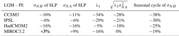
Table 2. LGM-PI changes in interannual variability of SLP in the Northern Hemisphere (σN H of SLP) and in the North Atlantic (σN Aof
SLP); fraction of variance explained by the leading EOF (λ1); amount of raw variability explained by the leading EOF in standard deviation
units ( q
λ1σN A2 ); and the amplitude of the seasonal cycle of Northern Hemisphere SLP variability (seasonal cycle of σN H). Standard
deviation changes that are not significant at 1% confidence level are in bold.
LGM – PI: σN H of SLP σN Aof SLP λ1
q
λ1σN A2 Seasonal cycle ofσN H
CCSM3 −10% −11% −34% −28% −38%
IPSL −6% −6% −29% −21% −30%
HadCM3M2 −16% −16% −5% −18% −25%
MIROC3.2 +3% +9% −16% 0% −19%
model, but also between models for simulations of a given climate. Both the ERA-40 (Uppala et al., 2005) and NCEP-NCAR (Kistler et al., 2001) reanalyses are used to validate general characteristics of the PI model results. A set of fig-ures analogous to the model results in Sect. 3, but using the ERA-40 reanalysis, is shown in Appendix A. Both reanalyses are used to validate model-based interpretations in Sect. 4. 3.1 Spatial distribution of SLP variance
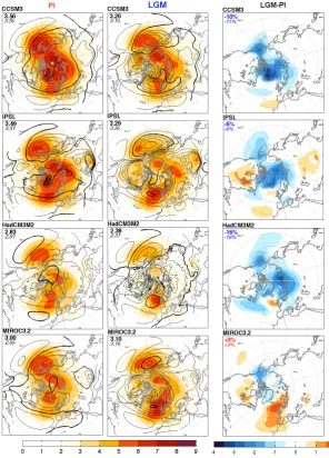
In three out of four models, the interannual variability of NH SLP is reduced in the LGM simulations compared to the PI simulations (Fig. 1). The differences in standard devia-tion (σ) are largest in high latitudes, especially along Green-land’s east coast, over the northeastern Pacific Ocean along the coast of Alaska, and over the Barents Sea (Fig. 1, right panels). Averaged over the extratropical NH, the model sim-ulations exhibit a significant LGM decrease in SLP standard deviation compared to the PI (Fig. 1), ranging from 6% in IPSL to 16% in HadCM3M2. MIROC3.2 shows a small and not significant increase in SLP standard deviation in the LGM simulation. Reductions in LGM interannual variability are also simulated for the free troposphere (500 hPa geopo-tential heights, not shown) and Li and Battisti (2008) docu-mented an analogous decrease in jet level wind variability in CCSM3’s LGM simulation.
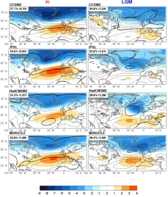
The leading mode of North Atlantic SLP variability from EOF analysis (Fig. 2) shows that an NAO-like feature is the leading mode of North Atlantic SLP variability in the LGM simulations, but it is less well-defined and represents less in-terannual variance than in the PI. The fraction of variance associated with the leading LGM mode (λ1) is reduced in all
models (Fig. 2 and Table 2). The CCSM3 exhibits the largest change inλ1from the PI (38%) to LGM (25%) simulation
andλ1values are similar to the extratropical NH winter
cal-culations reported by Otto-Bliesner et al. (2006) in the same simulations.
There is an LGM decrease of between 18 and 28% in the interannual SLP standard deviation associated with the lead-ing mode (
q
λ1σN A2 ) for each model except MIROC3.2. For
the three consistent models, the LGM decrease results from combined reductions in both interannual SLP variance (σN A2 ) and the fraction of variance explained by the leading mode of SLP variability (see Fig. 2 and Table 2). There is no change in the interannual SLP standard deviation explained by the leading mode in MIROC3.2, due to compensating changes in SLP variance and the fraction of variance explained by the leading mode.
Fig. 1. The mean (contours: 4 hPa interval from 1000 to 1040 hPa; higher values omitted for clarity; bold contour denotes 1016 hPa) and
standard deviation (colored shading: hPa) of monthly SLP averaged over all months in simulations of PI (left) and LGM (center) climate. Numbers show the SLP standard deviation area-averaged over the Northern Hemisphere (σN H in bold) and over the North Atlantic (σN Ain
italic). Differences (LGM-PI) are shown in the right panels.
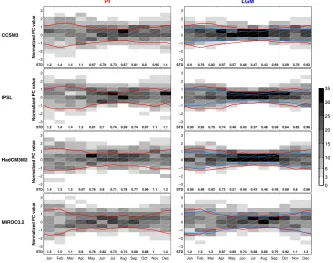
3.2 Seasonal cycle of variability
Reductions in interannual SLP variability within the LGM simulations relative to the PI simulations are not evenly dis-tributed throughout the year. Figure 3 shows the seasonal cy-cle of interannual SLP standard deviation for all model simu-lations. LGM reductions are concentrated in winter, the sea-son with the most interannual variability in each model’s sim-ulation of both climates. In summer and early fall, changes are smaller and often not statistically significant. The leading mode of SLP variability (Fig. 2) exhibits reductions in asso-ciated variance that are also concentrated in winter (Fig. 4), suggestive of a dynamically consistent model response dur-ing the most active season for North Atlantic variability.
Fig. 2. Leading EOF of monthly SLP anomalies (colored shading: hPa/standard deviation of PC) and SLP climatology (contours: 4 hPa
interval from 1000 to 1040 hPa; higher values omitted for clarity; bold contour denotes 1016 hPa) in the North Atlantic sector (all months) for the PI and LGM simulations. Numbers show the amount of variance explained by the first mode both as a percentage of the total variance
(λ1) and as a standard deviation in hPa ( q
λ1σN A2 ).
1 2 3 4 5 6 7 8 9 10 11 12 1.5
2 2.5 3 3.5 4 4.5 5
HadCM3M2
Months
1 2 3 4 5 6 7 8 9 10 11 12 1.5
2 2.5 3 3.5 4 4.5 5
IPSL
Months
1 2 3 4 5 6 7 8 9 10 11 12 1.5
2 2.5 3 3.5 4 4.5 5
MIROC3.2
Months
1 2 3 4 5 6 7 8 9 10 11 12 1.5
2 2.5 3 3.5 4 4.5 5
CCSM3
Area
−
averaged STD (hPa)
Months
ERA40 PI LGM
Fig. 3. Seasonal cycle of interannual SLP standard deviation over the Northern Hemisphere in the PI and LGM simulations, and for the
2 4 6 8 10 12 −3 −2 −1 0 1 2 3
Normalized PC value
CCSM3
PI
STD 1.2 1.4 1.4 1.1 0.97 0.79 0.73 0.67 0.81 0.9 0.95 1.1
2 4 6 8 10 12
−3 −2 −1 0 1 2 3 LGM
STD 0.9 0.76 0.82 0.67 0.57 0.48 0.47 0.43 0.69 0.69 0.76 0.82
2 4 6 8 10 12
−3 −2 −1 0 1 2 3
Normalized PC value
IPSL
STD 1.2 1.4 1.4 1.3 0.81 0.7 0.74 0.58 0.74 0.97 1.1 1.1
2 4 6 8 10 12
−3 −2 −1 0 1 2 3
STD 0.95 0.95 0.79 0.74 0.48 0.43 0.37 0.48 0.58 0.64 0.82 0.96
2 4 6 8 10 12
−3 −2 −1 0 1 2 3
Normalized PC value
HadCM3M2
STD 1.4 1.3 1.2 0.97 0.78 0.8 0.71 0.78 0.77 0.96 1.1 1.3
2 4 6 8 10 12
−3 −2 −1 0 1 2 3
STD 0.86 0.96 0.82 0.73 0.51 0.46 0.43 0.48 0.49 0.69 0.8 0.86
Jan Feb Mar Apr May Jun Jul Aug Sep Oct Nov Dec
−3 −2 −1 0 1 2 3
Normalized PC value
MIROC3.2
STD 1.5 1.5 1.1 0.9 0.78 0.82 0.73 0.74 0.68 0.88 1 1.4
Jan Feb Mar Apr May Jun Jul Aug Sep Oct Nov Dec
−3 −2 −1 0 1 2 3
STD 1.2 1.3 1.3 0.97 0.83 0.74 0.68 0.65 0.75 0.92 1.1 1.3
0 3 6 10 15 20 25 30 35
Fig. 4. The seasonality of NAO-like variability in LGM and PI simulations. For each month, the shading in each 0.5 standard deviation bin
(y-axis) represents the occurrence frequency of the NAOlike PC1 within that interval. The monthly PC1 time series from both simulations of a given model is normalized by the standard deviation of the annually averaged PC1 from the models PI simulation. This standardization enables a comparison between the models simulation of the two climate states. The spread of the normalized PC1s in a given month is an indication of the interannual variability in the leading mode for that month: a wider spread suggests that the amplitude of NAO-like oscillations is increased. The standard deviations of the PC in these normalized units are indicated along thex-axis for each month and are marked by the lines (red for PI, blue for LGM).
3.3 Discussion
The LGM simulations show a significant reduction in inter-annual SLP variance and a weakening of the leading mode of SLP variability relative to the PI simulations. These changes in atmospheric variability must be due to differences in radia-tive forcing, land/ocean geometry, land ice, and their com-bined influence on surface properties such as sea surface temperature and sea ice distribution. However, the details of these LGM-PI changes vary considerably from model to model, making it difficult to draw clear conclusions. In this section, we present results of some sensitivity experiments designed to address these issues, but the analyses and exper-iments required for a complete treatment of what causes the LGM-PI and model-to-model differences in SLP variability are beyond the scope of this study.
The sensitivity experiments were performed with the Community Atmosphere Model CAM3 (Collins et al., 2006), the atmospheric component of the CCSM3 coupled model. CAM3 is able to reproduce the climatology and variability of the full CCSM3 for each climate given the appropriate forcings: insolation, land mask, ice sheets (topography and albedo), greenhouse gas concentrations, as well as sea
sur-face temperature (SST) and sea ice fields from the ocean component of the coupled model (Figs. 5 and 6). The ex-periments, with their forcing setups, are listed in Table 3.
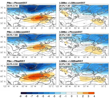
Fig. 5. The mean (contours: 4 hPa interval from 1000 to 1040 hPa;
higher values omitted for clarity; bold contour denotes 1016 hPa) and standard deviation (colored shading: hPa) of monthly SLP aver-aged over all months in the sensitivity experiments. Numbers show the SLP standard deviation area-averaged over the Northern Hemi-sphere (σN H in bold) and over the North Atlantic (σN Ain italic).
The sensitivity experiment with LGM external forc-ing (LGMbc+PIccsmSST) shows a mean SLP field that resembles the mean state of the full LGM simulation (LGMbc+LGMccsmSST), even when forced by PI SST/sea ice (Fig. 5). The leading mode of SLP variability in each LGM external forcing experiment is also quite similar to the full LGM simulation (Fig. 6), but the pattern of internannual SLP variability is different in each experiment (Fig. 5). The experiments using PI external forcing (PIbc+LGMccsmSST) have mean SLP distributions that resemble those of the full PI simulation, even when forced by LGM ocean forcing (SST and sea ice) (Fig. 5). The leading mode of SLP variabil-ity and its explained variance are also comparable to the full
Table 3. Boundary conditions (insolation, ice sheet and greenhouse
gases) and SST and sea ice forcings used for the sensitivity experi-ments.
Experiment Boundary Conditions (bc) SST + Sea Ice.
PIbc+LGMccsmSST PI LGM CCSM3
LGMbc+PIccsmSST LGM PI CCSM3
PIbc+PIhadSST PI PI HadCM3M2
LGMbc+LGMhadSST LGM LGM HadCM3M2
PI simulation (Fig. 6), while the pattern of interannual SLP variance is different in all three experiments (Fig. 5). In all the sensitivity experiments the leading mode variance is not consistently affected by the SST and sea ice (not shown).
There are a number of ways in which changes in the exter-nal forcing can affect atmospheric variability.We focus our discussion on ice sheets and greenhouse gases as these ex-hibit larger LGM-PI differences than insolation (see Fig. 1 in Otto-Bliesner et al., 2006). The large Laurentide ice sheet covering North America creates an upstream-blocking sit-uation that may be related to a stronger, but less variable, Atlantic jet at the LGM relative to the PI climate (Li and Battisti, 2008; Donohoe and Battisti, 2009). The reduced variance associated with the leading mode of SLP variability (Fig. 4) is broadly consistent with this change in upper-level jet variability; it could also be linked to the lower greenhouse gas concentrations at the LGM, much as the recent increase in NAO variance is thought be linked to external factors such as increases in greenhouse gas concentrations and/or changes in surface properties (Feldstein, 2002). Our results suggest that surface properties (SST and sea ice), are not important for determining the leading mode of SLP variability, but have some influence on the magnitude and pattern of interannual SLP variability. These findings are qualitatively consistent with the study of Kushnir et al. (2002), in which it is demon-strated that atmospheric variability is more affected by in-ternal atmospheric processes than by the extratropical ocean. Other studies suggest that sea ice anomalies can affect atmo-spheric variability, particularly the phase and amplitude of the NAO (Deser et al., 2000; Seierstad and Bader, 2008).
Fig. 6. Leading EOF of monthly SLP anomalies (colored shading: hPa/standard deviation of PC) and SLP climatology (contours: 4 hPa
interval from 1000 to 1040 hPa; higher values omitted for clarity; bold contour denotes 1016 hPa) in the North Atlantic sector (all months) for the sensitivity experiments. Numbers show the amount of variance explained by the first mode both as a percentage of the total variance
(λ1) and as a standard deviation in hPa ( q
λ1σN A2 ).
atmosphere model CAM3 produces similar SLP variability, regardless of the exact ocean forcing used, consistently with the results of the aforementioned sensitivity studies (PIbc+LGMccsmSST and LGMbc+PIccsmSST). A likely explanation is that the atmosphere models respond differ-ently to the same external forcing because of differences in the PI zonal mean flows simulated by the two coupled models, or perhaps because of differences in physics inter-nal to the two atmospheric models (e.g., differences in the parametrization of gravity wave drag). We can not rule out, however, that the atmosphere model used in the HadCM3M2 is more sensitive to the prescription of the ocean forcing than is the atmospheric model used in the CCSM3, and the differ-ences in the LGM mean state and variability simulated by the HadCM3M2 and the CCSM3 are symptomatic of the differ-ences in the SST and sea ice simulated in these two coupled models.
In summary, our findings suggest that the differences be-tween LGM and PI simulations in CCSM3 are due to the ex-ternal forcing, with the ocean forcing playing a minor role.
Reduced interannual variability at the LGM relative to the PI is a consistent change observed in several of the mod-els, and hence considered a robust model result. The ex-act amount and spatial charex-acteristics of this variability ap-pear to be model-specific.
4 Paleoclimate implications
Changes in the mean and variability of atmospheric circula-tion, in the leading modes, or in the seasonality of any of these components are interesting from a dynamical stand-point, but they could also have a demonstrable impact on the signal recorded in climate proxies.
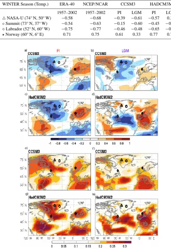
Table 4. Correlations between winter season surface air temperature and PC1 of sea level pressure in the North Atlantic sector for the four
locations indicated in Figs. 7 and 8. Correlations values from ERA-40 and NCEP/NCAR reanalysis are shown for comparison. The four locations have been chosen as reference points: the locations on Greenland have been widely used for climate reconstructions; the other two land points are areas where the models agree that temperature and/or precipitation variability are coherently related to the leading mode of variability in both climates.
WINTER Season (Temp.) ERA-40 NCEP/NCAR CCSM3 HADCM3M2
1957–2002 1957–2002 PI LGM PI LGM
4NASA-U (74° N, 50° W) −0.58 −0.68 −0.39 −0.61 −0.57 0.33
◦Summit (73° N, 37° W) −0.54 −0.63 −0.15 −0.60 −0.45 −0.08
Labrador (52° N, 60° W) −0.75 −0.77 −0.46 −0.48 −0.65 −0.55
?Norway (60° N, 6° E) 0.71 0.75 0.61 0.33 0.77 0.70
Fig. 7. PI and LGM correlations between North Atlantic winter surface air temperature (November to April) and PC1 (NAO-like index) for
CCSM3 (a), (b) and HadCM3M2 (c), (d). An indicator of temperature coherence in the sector for CCSM3 (e), (f) and HadCM3M2 (g),
(h): the value at each point is the absolute value of the area-averaged correlation between temperature at that point and the rest of the North
Fig. 8. Same as Fig. 7 for precipitation.
variability over recent centuries have been performed using archives such as tree rings (e.g. Glueck and Stockton, 2001), ice cores (e.g. Appenzeller et al., 1998) and pollen in lake sediments (e.g. Voigt et al., 2008). A common goal in se-lecting proxy sites is to find locations where local variability represents larger spatial scales. For example, in the present climate, surface temperature and precipitation at many lo-cations in the Atlantic sector are coherently coupled to the NAO (e.g. Hurrell, 1995), such that any site able to capture the leading mode of SLP variability (NAO) will also capture dynamically linked aspects of regional climate variability.
There have been studies attempting to reconstruct regional climate variability in different climate states from a limited number of locations (e.g. Allen et al., 1999; Bakke et al., 2005; Bahr et al., 2006). Unfortunately, the same geographic
site may record a qualitatively different mixture of mean and variance contributions in different climates. For example, the of atmospheric variability could change, resulting in a center of action shifting towards or away from a proxy site. Al-ternatively, a change in seasonality (i.e., in how variability is distributed throughout the year) could affect proxies that record signals preferentially at certain times of the year.
1 2 3 4 5 6 7 8 9 10 11 12 −15
−10 −5 0 5 10 15 20 25
NASA−U (74ºN 49.5ºW)
Month
Temperature (ºC)
2 4 6 8 10 12
−15 −10 −5 0 5 10 15 20 25
Month
Temperature (ºC)
SUMMIT (72.5ºN 37.5ºW)
2 4 6 8 10 12
−12 −10 −8 −6 −4 −2 0 2 4 6 8 10 12
Month
Precipitation (mm)
1 2 3 4 5 6 7 8 9 10 11 12
−10 −8 −6 −4 −2 0 2 4 6 8 10
Month
Precipitation (mm)
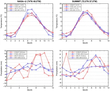
CCSM PI (28.5mm) CCSM LGM (9.5mm) HAD PI (29.0mm) HAD LGM (5.0mm)
CCSM PI (25.0mm) CCSM LGM (9.5mm) HAD PI (19.0mm) HAD LGM (6.0mm) CCSM PI (−23.4ºC) CCSM LGM (−34.4ºC) HAD PI (−27.5ºC) HAD LGM (−37.5ºC) CCSM PI (−19.6ºC)
CCSM LGM (−30.0ºC) HAD PI (−20.3ºC) HAD LGM (−34.9ºC)
Fig. 9. PI and LGM seasonal cycle for temperature (upper panels) and precipitation (lower panels) in CCSM3 and HadCM3M2 for two
locations in Greenland (NASA-U (left) and Summit (right)). The annual mean has been subtracted to facilitate comparison between climate states and models.
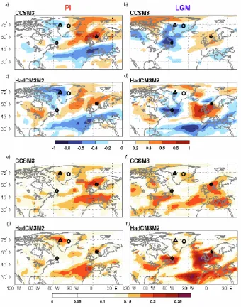
Fig. 10. Solid (dashed) lines represent the areas where the correlation between temperature (precipitation) and the PC1 of the SLP for all the
models is greater than 0.4 in absolute value in the PI and LGM simulations.
both temperature and precipitation (Figs. 7–8 panels e and g). In contrast, the pattern of variability during the LGM is model dependent, but in each model different from that in the PI simulations (Figs. 7–8 panels f and h).
The link between surface climate variability and the lead-ing mode of SLP variability can also be altered in a dif-ferent climate state: that is, the relationship between sur-face climate and the leading mode of SLP variability can change. Correlation statistics between surface temperature or precipitation and the temporal series of the leading mode
between the leading mode of SLP variability and surface climate variability. Two behaviors emerge from the model analysis: (1) for CCSM3, surface climate variability in the North Atlantic is not dominated by the leading (NAO-like) mode of SLP variability (compare panels b and f in Figs. 7 and 8); (2) for HadCM3M2, surface climate is more strongly linked to NAO-like variability (compare panels d and h in Figs. 7 and 8). CCSM3 shows a much larger reduction in the strength of NAO-like variability relative to HadCM3M2 in the LGM simulations (Fig. 2 and Table 2), which could be the reason for the disagreement between the models.
Figures 7 and 8 show that because of changes in the link between the of leading mode of SLP variability and sur-face climate, a location might be able to record the leading mode but not reflect regional surface climate variability at the LGM. As one example, regional variability may be dis-connected from the leading mode of SLP, as seen for Sum-mit, Greenland in the CCSM3 (compare panels b and f in Figs. 7 and 8). Another possibility is that because of the southward shift of the leading mode of SLP variability at the LGM, Greenland might be situated at the flank of the dom-inant North Atlantic atmospheric variability in a glacial cli-mate. An example of this is that surface climate at the Sum-mit of Greenland in HadCM3M2 reflects a combination of both regional and leading mode variability in the PI (panels c and g in Fig. 7, Table 4), but not in the LGM (panels d and h in Fig. 7).
Finally, changes in the seasonality of surface climate vari-ability might cause an altered signal recorded by proxies (Krinner and Werner, 2003). Figure 9 shows how the mag-nitude of the seasonal cycle varies for two ice core locations in Greenland during the LGM compared to PI: the seasonal cycle of temperature is enhanced at the station NASA-U in the LGM simulations, whereas it is comparable at Summit; the seasonal cycle of precipitation is substantially modified at both locations. Neglecting this change in seasonality might cause a bias in LGM temperature estimates based on water isotopes, since theδ18O signal recorded at the LGM would have a different seasonal imprint than during the PI (Steig et al., 1994; Krinner and Werner, 2003).
Our study shows how assuming modern climate relation-ships for past climates can produce erroneous interpretations of paleoclimate records. Modelers must also be cautious when interpreting simulations of the LGM, given that the models are not able to depict a consistent spatial pattern of surface climate or SLP variability in this climate state. In a few areas where the models do agree, it is possible to infer that in both climates a substantial amount of regional vari-ability of either temperature or precipitation can be reliably reproduced, for example in southern Norway (Table 4 and Figs. 7 and 8) or in Labrador (Fig. 10, Table 4).
5 Conclusions
In this paper, we analyze surface climate variability in the extratropical North Atlantic using LGM and PI simulations from four climate models. We describe how changes in at-mospheric variability may affect signals recorded by proxies. The main findings are:
– The interannual variability of Northern Hemisphere sea level pressure (SLP) is significantly reduced at the LGM.
– The seasonal cycle of sea level pressure variability is de-creased during the LGM. The reduction is more promi-nent and significant in the winter months, when the vari-ability is highest in both the PI and LGM climates. – An NAO-like pattern is the leading mode of SLP
vari-ability in each LGM simulation examined, though it represents less interannual variability and the centers of action are weaker.
– The ice sheets and greenhouse gases largely determine the mean circulation and the amplitude of the leading mode of variability, while the SST/sea ice help to de-termine the amount of SLP variability. Different atmo-spheric models respond differently to the same ice sheet and greenhouse gas forcings, so simulated differences in the pattern and amplitude of the leading mode of SLP variability (NAO-like) appear to be sensitive to different model’s physics and/or parameterizations.
– The relationship between atmospheric variability and surface climate variability is different during the LGM. Therefore, caution is necessary when interpreting proxy records using the modern relationship as an analog.
Appendix A
In order to compare the PI simulations with modern obser-vations, the same analyses have been performed using the ERA-40 reanalysis and are shown in Fig. A1.
Acknowledgements. This work is part of the ARCTREC project
a)
c) d)
b)
Jan Feb Mar Apr May Jun Jul Aug Sep Oct Nov Dec
−3 −2 −1
0
1 2 3
Normalized PC value STD 1.6 1.6 1.5 0.86 0.66 0.76 0.62 0.77 0.63 0.85 0.95 1.2 0
3
6
10 15 20 25 30 35
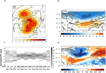
Fig. A1. ERA-40 reanalysis for the period 1957–2002; (a) The mean (contours) and standard deviation (colored shading: hPa) of monthly
SLP averaged over all months; (b) Leading EOF of monthly SLP anomalies (colored shading: hPa/standard deviation of PC) and SLP climatology (contours) in the North Atlantic sector (all months). Number shows the amount of variance explained by the first mode as a percentage of the total variance (λ1); in both panels the contours have 4 hPa interval from 1000 to 1040 hPa, bold contour denotes 1016 hPa; (c) Histogram of the leading principal component (PC1) of SLP as a function of month. For each month, the PC has been normalized by the
standard deviation of the annually averaged PC1. The standard deviations of the PC in these normalized units are indicated along thex-axis for each month and are marked by the lines; (d) Correlations between North Atlantic winter surface air temperature and PC1.
Colorado, USA, from their Web site at http://www.cdc.noaa.gov/. This paper is Bjerknes Centre for Climate Research contribution number A 250.
Edited by: M. Crucifix
References
Allen, J. R. M., Brandt, U., Brauer, A., Hubberten, H. W., Huntley, B., Keller, J., Kraml, M., Mackensen, A., Mingram, J., Negen-dank, J. F. W., Nowaczyk, N. R., Oberhansli, H., Watts, W. A., Wulf, S., and Zolitschka, B.: Rapid environmental changes in southern Europe during the last glacial period, Nature, 400, 740– 743, 1999.
Appenzeller, C., Schwander, J., Sommer, S., and Stocker, T. F.: The North Atlantic Oscillation and its imprint on precipitation and ice accumulation in Greenland, Geophys. Res. Lett., 25, 1939– 1942, 1998.
Bahr, A., Arz, H., Lamy, F., and Wefer, G.: Late glacial to Holocene paleoenvironmental evolution of the Black Sea, reconstructed with stable oxygen isotope records obtained on ostracod shells, Earth Planet. Sci. Lett., 241, 863–875, 2006.
Bakke, J., Lie, O., Nesje, A., Dahl, S., and Paasche, O.: Utiliz-ing physical sediment variability in glacier-fed lakes for contin-uous glacier reconstructions during the Holocene, northern Fol-gefonna, western Norway, Holocene, 15, 161–176, 2005. Braconnot, P., Otto-Bliesner, B., Harrison, S., Joussaume, S.,
Pe-terchmitt, J.-Y., Abe-Ouchi, A., Crucifix, M., Driesschaert, E., Fichefet, T., Hewitt, C. D., Kageyama, M., Kitoh, A., Laine, A., Loutre, M.-F., Marti, O., Merkel, U., Ramstein, G., Valdes, P., Weber, S. L., Yu, Y., and Zhao, Y.: Results of PMIP2 coupled simulations of the Mid-Holocene and Last Glacial Maximum – Part 1: experiments and large-scale features, Clim. Past, 3, 261– 277, 2007.
Collins, W. D., Rasch, P. J., Boville, B. A., Hack, J. J., McCaa, J. R., Williamson, D. L., Briegleb, B. P., Bitz, C. M., Lin, S. J., and Zhang, M. H.: The formulation and atmospheric simulation of the Community Atmosphere Model version 3 (CAM3), J. Cli-mate, 19, 2144–2161, 2006.
Dansgaard, W., Johnsen, S. J., Clausen, H. B., Dahjensen, D., Gun-destrup, N. S., Hammer, C. U., Hvidberg, C. S., Steffensen, J. P., Sveinbjorndottir, A. E., Jouzel, J., and Bond, G.: Evidence for General Instability of Past Climate from a 250-Kyr Ice-core Record, Nature, 364, 218–220, 1993.
Deser, C., Walsh, J. E., and Timlin, M. S.: Arctic sea ice variability in the context of recent atmospheric circulation trends, J. Cli-mate, 13, 617–633, 2000.
Donohoe, A. and Battisti, D. S.: Causes of reduced North Atlantic Storm Activity in a CCSM3 simulation of the Last Glacial Max-imum, personal communication, 2009.
Feldstein, S. B.: The recent trend and variance increase of the an-nular mode, J. Climate, 15, 88–94, 2002.
Gladstone, R., Ross, I., Valdes, P., Abe-Ouchi, A., Braconnot, P., Brewer, S., Kageyama, M., Kitoh, A., Legrande, A., Marti, O., Ohgaito, R., Otto-Bliesner, B., Peltier, W., and Vettoretti, G.: Mid-Holocene NAO: A PMIP2 model intercomparison, Geo-phys. Res. Lett., 32, L16707, doi:{10.1029/2005GL023596}, 2005.
Glueck, M. F. and Stockton, C. W.: Reconstruction of the North At-lantic Oscillation, 1429-1983, Int. J. Climatol., 21, 1453–1465, 2001.
Hurrell, J. W.: Decadal Trends in the North Atlantic Oscillation - Regional Temperatures and precipitation, Science, 269, 676– 679, 1995.
Hutterli, M. A., Raible, C. C., and Stocker, T. F.: Reconstructing climate variability from Greenland ice sheet accumulation: An ERA40 study, Geophys. Res. Lett., 32, 2005.
Jouzel, J., Lourius, C., Johnsen, S., and Grootes, P.: Climate Insta-bilities – Greenland and Antarctic Records, Comptes Rendus De l’ Academie Des Sciences Serie II, 319, 65–77, 1994.
Justino, F. and Peltier, W.: The glacial North Atlantic Oscillation, Geophys. Res. Lett., 32, L21803, doi:{10.1029/2005GL023822}, 2005.
Kistler, R., Kalny, E., and Collins, W.: The NCEP-NCAR 50-year reanalysis: monthly means CD-ROM and documentation , Bull. Am. Meteor. Soc., 82, 247–268, 2001.
Krinner, G. and Werner, M.: Impact of precipitation seasonality changes on isotopic signals in polar ice cores: a multi-model analysis, Earth Planet. Sci. Lett., 216, 525–538, 2003.
Kushnir, Y., Robinson, W. A., Blade, I., Hall, N. M. J., Peng, S., and Sutton, R.: Atmospheric GCM response to extratropical SST anomalies: Synthesis and evaluation, J. Climate, 15, 2233–2256, 2002.
Laˆın´e, A., Kageyama, M., Salas-M`elia, D., Voldoire, A., Rivi´ere, G., Ramstein, G., Planton, S., Tyteca, S., and Petershmitt, J. Y.: Northern hemisphere storm tracks during the last glacial maxi-mum in PMIP2 ocean-atmosphere models, J. Climate, 2008. Li, C. and Battisti, D. S.: Reduced Atlantic storminess during Last
Glacial Maximum: Evidence from a coupled climate model, J. Climate, 2008.
Miller, R. L., Schmidt, G. A., and Shindell, D. T.: Forced annu-lar variations in the 20th century intergovernmental panel on cli-mate change fourth assessment report models, J. Geophys. Res.-Atmos., 111, D18101, doi:10.1029/2005JD006323, 2006. Otto-Bliesner, B. L., Brady, E. C., Clauzet, G., Tomas, R., Levis, S.,
and Kothavala, Z.: Last Glacial Maximum and Holocene climate in CCSM3, J. Climate, 19, 2526–2544, 2006.
Peltier, W. and Solheim, L.: Dynamics of the ice-age Earth: Solid mechanics and fluid mechanics, J. Phys. IV, 12, 85–104, 2002. Peltier, W. R.: Global glacial isostasy and the surface of the ice-age
earth: The ice-5G (VM2) model and grace, Annu. Rev. Earth Pl. Sc., 32, 111–149, 2004.
Raible, C. C. Casty, C., Luterbacher, J., Pauling, A., Esper, J., Frank, D. C. Buntgen, U., Roesch, A. C., Tschuck, P., Wild, M., Vidale, P. L., Schar, C., and Wanner, H.: Cli-mate variability-observations, reconstructions, and model simu-lations for the Atlantic-European and Alpine region from 1500– 2100 AD, Clim. Change, 79, 9–29 , 2006.
Seierstad, I. A. and Bader, J.: Impact of a projected fu-ture Arctic Sea Ice reduction on extratropical
stormi-ness and the NAO, Clim. Dynam., available at:
http://www.springerlink.com/content/f843225242338024/ ?p=2e6e7fd67641427d82db0a37aaae483d&pi=4, 2008. Shackleton, N.: Paleoclimate – Climate change across the
hemi-spheres, Science, 291, 58–59, 2001.
Shindell, D. T., Miller, R. L., Schmidt, G. A., and Pandolfo, L.: Simulation of recent northern winter climate trends by greenhouse-gas forcing, Nature, 399, 452–455, 1999.
Steig, E. J., Grootes, P. M., and Stuiver, M.: Seasonal Precipitation Timing and Ice Core Rrecords, Science, 266, 1885–1886, 1994. Uppala, S. M., Kallberg, P. W., Simmons, A. J., Andrae, U.,
Bech-told, V. D., Fiorino, M., Gibson, J. K., Haseler, J., Hernandez, A., Kelly, G. A., Li, X., Onogi, K., Saarinen, S., Sokka, N., Al-lan, R. P., Andersson, E., Arpe, K., Balmaseda, M. A., Beljaars, A. C. M., Van De Berg, L., Bidlot, J., Bormann, N., Caires, S., Chevallier, F., Dethof, A., Dragosavac, M., Fisher, M., Fuentes, M., Hagemann, S., Holm, E., Hoskins, B. J., Isaksen, L., Janssen, P. A. E. M., Jenne, R., McNally, A. P., Mahfouf, J. F., Morcrette, J. J., Rayner, N. A., Saunders, R. W., Simon, P., Sterl, A., Tren-berth, K. E., Untch, A., Vasiljevic, D., Viterbo, P., and Woollen, J.: The ERA-40 re-analysis, Q. J. Roy. Meteor. Soc., 131, 2961– 3012, 2005.