www.nonlin-processes-geophys.net/14/361/2007/ © Author(s) 2007. This work is licensed
under a Creative Commons License.
Nonlinear Processes
in Geophysics
Observations of linear and nonlinear processes in the foreshock
wave evolution
Y. Narita1, K.-H. Glassmeier1,2, M. Fr¨anz2, Y. Nariyuki3, and T. Hada3
1Institute of Geophysics and Extraterrestrial Physics, Technical University of Braunschweig, Mendelssohnstr. 3, 38106 Braunschweig, Germany
2Max-Planck-Institute for Solar System Research, Max-Planck-Str. 2, 37191 Katlenburg-Lindau, Germany 3Department of Earth System Science and Technology, Kyushu University, 816-8580, Kasuga, Japan Received: 28 March 2007 – Revised: 2 July 2007 – Accepted: 2 July 2007 – Published: 9 July 2007
Abstract. Waves in the foreshock region are studied on the basis of a hypothesis that the linear process first excites the waves and further wave-wave nonlinearities distribute scatter the energy of the primary waves into a number of daughter waves. To examine this wave evolution scenario, the disper-sion relations, the wave number spectra of the magnetic field energy, and the dimensionless cross helicity are determined from the observations made by the four Cluster spacecraft. The results confirm that the linear process is the ion/ion right-hand resonant instability, but the wave-wave interactions are not clearly identified. We discuss various reasons why the test for the wave-wave nonlinearities fails, and conclude that the higher order statistics would provide a direct evidence for the wave coupling phenomena.
1 Introduction
1.1 Origin of foreshock waves
The physics of the collisionless shock waves is one of the most interesting subjects in space plasma. While the shock waves in the ordinary gas dynamics dissipate the kinetic en-ergy of the supersonic flow into the heat on a scale within a few mean free paths of particles, the collisionless shock waves exhibit a variety of dissipation mechanisms in a dilute plasma. When the flow speed is sufficiently large compared to the Alfv´en speed, the collisionless shock waves specularly reflect a portion of the incoming charged particles (super-critical shock). The reflected particles either gyrate about the magnetic field just in front of the shock wave when it is quasi-perpendicular to the shock normal direction, or stream toward upstream along the magnetic field when the field is quasi-parallel to the shock normal. In the latter case the
Correspondence to: Y. Narita
reflected particles form a field-aligned beam against the in-coming flow. Although both the ions and the electrons can be reflected at the shock, the ions play more important roles in the shock dissipation. This is because the ions carry the most of energy and momentum in the plasma. The back-streaming ions “warn” the upstream plasma about the exis-tence of the shock wave, and brake the upstream flow a little before it reaches the shock wave. The back-streaming ions encounter the incoming ion population and they form an un-stable beam-beam velocity distribution (the incoming and the reflected ions). The upstream plasma is therefore subject to waves and turbulence in order to relax the unstable velocity distribution. The region where the back-streaming ions exist is called the foreshock, which is often accompanied by fluc-tuations of the magnetic field and the plasma. The foreshock itself belongs to one of the dissipation mechanisms of the col-lisionless shock waves and provides pre-thermalization pro-cesses before the plasma stream reaches the shock wave.
1.2 Stage 1 – parent wave excitation
We assume that the primary waves are excited by the ion/ion right-hand resonant instability for the following reasons. In the linearized Vlasov equation model, the field-aligned ion beam injected into a plasma is subject to three kinds of elec-tromagnetic micro-instabilities: right-hand resonant, left-hand resonant, and non-resonant ion/ion instabilities. Here the term “ion/ion” means the core ions and the beam ions. These instabilities are well documented by Gary (1993). These instabilities are linear in the sense that the fluctuation amplitude (or the envelope of the fluctuation) grows expo-nentially as a function of time.
The right-hand instability stems from a resonance between the ion beam and the right-hand circularly polarized wave and it is the fastest growing under typical foreshock parame-ters. The instability excites the waves propagating along the magnetic field. The waves follow the magnetosonic/whistler branch in the dispersion relation, which becomes the Alfv´en waves at the small wave number limit. Here we mean the Alfv´en waves by the ones that satisfy the dispersion rela-tionω=kkVA, whereωdenotes the frequency, kkthe wave
number parallel to the mean magnetic field, and VA the Alfv´en speed. The maximum growth rate is typically at the wave number|kkVA/ p|≈0.1, where p denotes the ion cyclotron frequency. We assume protons for the ions (sub-script p). In observations the waves are often termed as the Alfv´en waves, as they propagate along the background mag-netic field. The experimentally determined dispersion rela-tions confirm the magnetosonic/whistler branch (Narita et al., 2003; Narita and Glassmeier, 2005).
The resonance between the left-hand polarized waves and the ion beam is also possible, but it is easier to excite the right-hand mode under cool beam conditions because at the low thermal velocities of the beam there are only few ions which can resonate with the left-hand mode. While the right-hand and the left-right-hand resonant modes excite waves paral-lel to the ion beam direction, the non-resonant mode excites waves in the opposite direction. The non-resonant mode is basically a firehose instability, caused by the inertia of the fast ion beam exerting a centrifugal force on the bent mag-netic field. This mode has a larger threshold to grow, since it has to overcome the restoring forces of perpendicular pres-sure.
1.3 Stage 2 – daughter wave excitation
When the primary wave amplitude exceeds a certain thresh-old, excess power spills into the daughter waves at the ex-pense of the primary wave. If the amplitude is increased further, the daughter waves generate further daughter waves successively. Hence doubling the wave amplitude may not be stable any more but result in a cascade of daughter waves. Such a process represents the wave-wave nonlinearities and is referred to as the parametric instabilities.
The parametric instabilities themselves exhibit different processes between the high and the low β regimes, where β=pt h/pm, the ratio of the thermal to the magnetic pres-sure. The decay of circularly polarized, parallel-propagating Alfv´en waves with respect to the mean magnetic field through the nonlinear interaction was first suggested by Galeev et al. (1963) and Sagdeev and Galeev (1969), where a parent Alfv´en wave collapses into plasma density fluctua-tions and a backward-propagating daughter Alfv´en wave (de-cay instability). This process was studied in detail using dis-persion relations for ideal magnetohydrodynamics (MHD) (Derby, 1978; Goldstein, 1978). However, Alfv´en waves are also subject to “modulational instability”, where all the daughter waves propagate in the same direction as the parent wave (Mio et al., 1976; Mjølhus, 1976; Nariyuki and Hada, 2006a). These two instability processes have been system-atically studied in the framework of the Hall-MHD (Longtin and Sonnerup, 1986; Terasawa et al., 1986; Wong and Gold-stein, 1986) and it was found that the dispersion plays an important role and the different instability processes prefer different plasmaβ regimes. While the decay instability is more characteristic to the lowβconditions, the modulational instability dominates under the high-β conditions. Forβ of the order of unity (β'1) the beat instability plays also an important role (Hollweg, 1994).
For simplicity we assume the following scenario for the second stage of the foreshock wave evolution. The parent wave excited at the first stage by the right-hand resonant in-stability is subject to the decay inin-stability, generating back-ward propagating waves (with respect to the parent wave di-rection) in the lowβregime, while it is subject to the modu-lational instability, generating forward propagating waves in the highβ regime (modulational instability). Therefore the cascade of the daughter waves results in both forward and backward propagating waves in the lowβ regime, and only forward in the highβ regime.
1.4 Cross helicity
Examination on the above scenario is conveniently made by investigating the cross helicity density, defined as
hc=v· B √
µ0ρ0, (1)
wherev,B,µ0, ρ0denote the flow velocity, the magnetic field, the permeability of free space, and the background mass density, respectively. The cross helicity density mea-sures the correlation between the velocity and the magnetic field fluctuations, and its magnitude is maximized when the fluctuations are the Alfv´enic, v∝±B. We introduce the Els¨asser variables
z±=v±√B
in which case the cross helicity density is written in the form
hc=E+−E−, (3)
whereE±=|z±|2. This means that the cross helicity is essen-tially a measure of the energy difference between the two op-positely propagating Alfv´en waves. The cross helicity den-sity can be normalized to unity as
σc=
E+−E−
E++E−. (4)
For example,σc=1 means the presence of the forward prop-agating (e.g. parallel to mean magnetic field) only, and vice versa. In the following we callσcsimply the cross helicity. 1.5 Test for the hypothesis
To test the hypothesis for the foreshock waves we assume the Alfv´enic fluctuations and determine the cross helicityσc using the four point magnetic field data in the foreshock re-gion ahead of the terrestrial bow shock. The cross helicity is investigated under various conditions ofβ. We expect from the hypothesis that the cross helicity is dependent on the val-ues ofβ. The diminished cross helicity for lowerβ and the enhanced cross helicity for higherβ, which results from the wave-wave interaction model at the second stage of the wave evolution.
In Sect. 2 we give brief introductions of the wave analysis methods: the dispersion relations, the wave number spectra, and the cross helicity. Those who are familiar with these methods may skip into Sect. 3, where we present the statistics of the cross helicity and its dependence onβ.
2 Wave analysis
2.1 Wave telescope estimator
The four point measurements enable one to determine the spectral density matrix as function of frequencyωand wave vectork,
E(ω,k)=
Exx ExyExz Eyx EyyEyz Ezx Ezy Ezz
. (5)
While it is straightforward to determine the fluctuation am-plitude atωsimply by Fourier transforming the time series data, the amplitude atkis not easily obtained by the Fourier transform procedure because of the limited number of the measurement points. It is, however, possible to determine the matrix E(ω,k)when applying the so-called wave telescope estimator,
E(ω,k)=hV†H†M−1H Vi
−1
. (6)
Here the matrix M is the 12×12 cross spectral density ma-trix a function of frequency. It is determined by the measure-ments of the magnetic field fluctuations as
M(ω)= 1
1ωhBB
†i, (7)
where the symbolh··idenotes the ensemble average and the dagger † means the Hermitian conjugate. M consists of the incorporated vectorB for each component of the magnetic field fluctuations (the x-, y-, and z-directions) and for each measurement point (spacecraft 1,· · ·,4),
B(ω)=
b1x b1y .. . b4z
. (8)
The matrix H is called the steering matrix, as it steers the output matrix E for various wave vectorsk, and defined as
H(k)=
Ieik·r1
Ieik·r2
Ieik·r3
Ieik·r4
, (9)
where I denotes the 3×3 unit matrix, andrithe position vec-tor of the measurements. The matrix V imposes a further constraint on the spectral matrix, reflecting the fact that the magnetic field is divergence-free. It is defined as
V(k)=I+kk
†
k2 , (10)
where k=|k|. Its algorithm was tested on simulated data to retrieve the input model. See, for example, Pinc¸on and Lefeuvre (1991); Motschmann et al. (1996) and Glassmeier et al. (2001). Derivation of Eq. (6) is shown in Appendix A.
We choose a coordinate system with the z axis aligned to the mean magnetic field direction. The z axis is parallel to the mean field when its sunward component is positive, and vice versa, so that the z-axis is always oriented in the direction away from the bow shock. We use the Earth-to-sun direction projected into the plane perpendicular to the mean field as the x-axis. Namely, our coordinate system is spanned by the following unit vectors
ex=ey×ez (11)
ey=esun×eb (12)
ez= Bx
|Bx|
eb, (13)
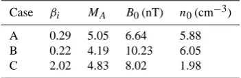
Table 1. The ion beta, the Alfv´en Mach number, the mean magnetic field strength, and the plasma density.
Case βi MA B0(nT) n0(cm−3)
A 0.29 5.05 6.64 5.88
B 0.22 4.19 10.23 6.05
C 2.02 4.83 8.02 1.98
2.2 Dispersion relations
One of the useful applications of the wave telescope estima-tor is to determine the dispersion relations from the observa-tions. We compute the total wave powere(ω,k)by taking trace of the matrix E,
e(ω,k)=tr E. (14)
We investigate the total wave powereat various frequencies (in the spacecraft frame of reference) and wave vectors, and identify the pairs of the frequency and the wave vector which yield peaks in the total wave power. It is worthwhile to note that the wave telescope estimator assumes the fluctuations as a set of incoherent wave fields, and therefore it is subject to interference, for example, when two waves possess exactly the same frequency. The frequencies can be transformed from the spacecraft frame frequencyωsc to the plasma rest frame frequencyωre(co-moving with the plasma bulk flow) using the Doppler relationωre=ωsc−k·V0, whenkis deter-mined by the wave telescope method andV0(the mean flow velocity vector) is known.
We apply the dispersion analysis to the measurements pro-vided by the four Cluster spacecraft (Escoubet et al., 2001). The magnetic field measurements of the FGM instrument (Balogh et al., 2001) are used to determine the pairs of the frequency and the wave vector, and the ion measurements of the CIS-HIA instrument (R`eme et al., 2001) are used to determine the mean flow velocity. Various kinds of curves of the dispersion relations are identified in the foreshock re-gion by this analysis. Figure 1 displays three distinct cases of the dispersion curves for the field-aligned wave numbers, ωre(kz). Hereafterωreis normalized to the proton cyclotron frequencyp, andkzis normalized to the ion inertial wave number p/VA. The Alfv´en speed is determined by the magnetic field and the ion measurements for each time in-terval. Table 1 summarizes the plasma and magnetic field parameters for the three cases: the ion betaβi(assuming pro-tons); the Alfv´en Mach numberMA; the mean magnetic field strengthB0; and the plasma densityn0.
In the case A (16 February 2002, 07:00–07:30 UT) almost all of the waves are identified in the direction away from the shock. Only few waves propagate in the opposite direction at very low frequencies (ωre'0). The dispersion branch starts at(ωre, kz)=(0,0)and extends solely in the anti-parallel
di-rection, keeping the phase speed almost at the Alfv´en speed vA at low frequencies,ωre/ kz'vA. Atωre∼0.5 the disper-sion branch starts to be bent and deviates from the linear branch toward higher frequencies. This is characteristic to the low frequency part of the magnetosonic/whistler waves.
The case B (27 April 2002, 02:00–02:30 UT) exhibits waves that are counter-propagating at low frequencies. Most of the identified waves propagate in the+zdirection at var-ious frequencies (ωre≤3), but some waves propagate in the opposite direction at low frequencies (ωre≤0.4). The disper-sion branch in the+zdirection, can be approximated by a straight line (linear dispersion relation), but the phase speed does not agree with the Alfv´en speed (ωre≥kzvA). In the−z direction it is not clear if the waves follow any dispersion relation, since only few waves are identified.
The case C (6 March 2002, 00:30–01:00 UT) exhibits an example of the enhanced counter-propagating waves. Compared to the case B, the identified waves look rather scattered in the dispersion diagram. One branch starts at (ωre, kz)'(0,0) and extends in the +z direction to (ωre, kz)=(3,−1.5), while the branch in the −z direc-tion stops at ωre'1.5. The scatter in the dispersion di-agram makes it difficult to identify the dispersion rela-tion, but roughly speaking, the waves follow the magne-tosonic/whistler branch.
2.3 Wave number spectra
The second application of the wave telescope estimator is the wave number spectra (energy spectra in the wave num-ber domain). We determine two kinds of wave numnum-ber spec-tra: E+(kz)andE−(kz). They represent the energy for the Alfv´enic fluctuations propagating along the magnetic field away from the shock (E+), and toward the shock (E−),
re-spectively, and are determined as follows.
E+(kz)= α 1k
Z dωre
Exx(ωre, kz)+Eyy(ωre, kz)
(15) E−(kz)=
α 1k
Z dωre
Exx(ωre,−kz)+Eyy(ωre,−kz)
, (16) where the integration is made over the frequency in the plasma rest frame.
Fig. 1. Wave frequencies in the plasma rest frame and wave num-bers aligned to the mean magnetic field. The+zdirection is away from the shock toward upstream.
in the time domain for the normalization, assuming that the fluctuations are homogeneous.
The wave number spectra for the three cases A, B, and C are displayed in Fig. 2. The wave numbers are scaled
Fig. 2. Energy spectra of the Alfv´enic fluctuations in the wave num-ber domain for the wave numnum-ber away from the shock (solid curve) and for the wave number toward the shock (dotted curve).
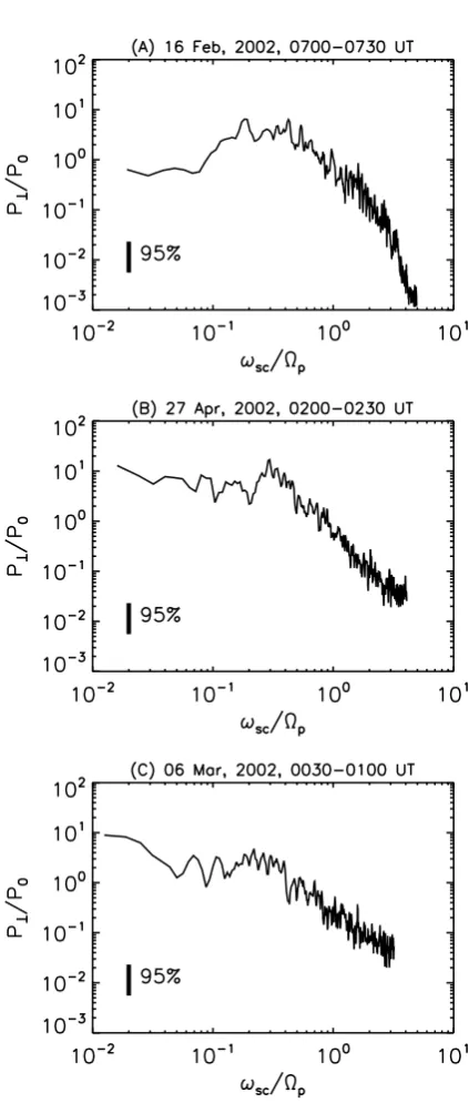
Fig. 3. Energy spectra of the magnetic field fluctuations perpendic-ular to the mean field in the frequency domain.
line), that is the foreshock fluctuations contain more energy in the waves propagating away from the shock than that for the waves toward the shock. Another point is that the spectra exhibit humps which are an indication of the energy injec-tion. The humps can be seen only inE+, whileE−shows only monotonously decaying curves toward the larger wave numbers. The injection scale is, however, slightly different from case to case. It becomes shifted gradually toward the
larger wave numbers from the case A to the case C. A closer inspection yields the values of the normalized wave num-bers for the injection scales:kz≈0.05−0.1 (case A); 0.1−0.2 (case B); and 0.3 (case C). The difference betweenE+and E−becomes also smaller from the case A to the case C. Frequency spectra
For comparison, frequency spectra for the three events are displayed in Fig. 3, where the wave power for the mag-netic field fluctuation perpendicular to the mean fieldP⊥is
scaled usingP0=2π B02VA/V0p and the spacecraft frame frequency is scaled to the proton cyclotron frequency. It is important to note that one cannot distinguish betweenE+ andE− from the magnetic field measurements only in the frequency spectra. Of course, the frequency spectra can be determined using the Els¨asser variables, but still one cannot reach smaller scales due to the limited sampling rate for the particle measurements, which is typically the time scale of the spacecraft spin, a few seconds. The frequency spectra exhibit more or less resemblance to the wave number spec-tra. But this is not surprising, as the solar wind streams at the supersonic and super-Alfv´enic speed and the spatial struc-tures are recorded as the temporal variations by the space-craft. However, the frequency spectra exhibit spikes on vari-ous scales. Some are small scale, sharp spikes and some are large scale, blunt spectral hump. Generally speaking, it is difficult to identify the energy injection scale and the power-law decay of the spectra unambiguously.
2.4 Dimensionless cross helicity
The third application of the wave telescope estimator is the dimensionless cross helicityσc. We apply the two energy spectraE+andE− as determined in Eqs. (15) and (16) to the Eq. (4). In our coordinate systemE+denotes the waves propagating away from the shock, henceσc=1 means that all the Alfv´enic fluctuation energy represents waves propagating in this direction.
helicity also agrees with the energy injection scale obtained in the previous section.
3 Statistical study
3.1 Event selection
The dimensionless cross helicityσc is investigated for vari-ous time intervals of the observations in the foreshock region. Following criteria are imposed to select the time intervals for the foreshock wave observations: (1) mission phase with the smallest inter-spacecraft distance, 100 km, to resolve as smallest wavelengths as possible (February to May 2002), (2) existence of supra-thermal ion populations, namely back-streaming ions in addition to the solar wind ion population, (3) enhanced level of magnetic field fluctuations. We select the time intervals with the fluctuating energy more than 30% of the mean field energy,
*
|δBx|2+ |δBy|2+ |δBz|2 B02
+1/2
≥0.3, (17)
whereδBx,δBy, andδBzdenote the three components of the fluctuating magnetic field, andB0denotes the mean magnetic field strength. The mean field is defined by averaging the field strengthB0=hBiso thatB0can be treated as a uniform constant vector for each 30 min interval. The ion measure-ments of the CIS-HIA instrument are used in step (2). As a result we obtain 32 intervals for the statistical study. 3.2 Distribution of cross helicity
Figure 5 displays the superposed cross helicity for all the events. As the three case studies show in the previous section, the cross helicity is positive at various wave numbers. Statis-tically the foreshock is indeed dominated by the waves prop-agating away from the shock. On the largest scale (kz∼0.01, wherekzis normalized to the ion inertial scale) the cross he-licity approaches to zero. At the wave numberskz∼0.1 the cross helicity reaches its maximum, but the distribution of the maximum cross helicity ranges from almost zero to al-most unity. On the smaller scales (kz>1) the cross helicity is diminished. We estimate the injection scale of the cross helicity for the wave numbers yielding the maximum cross helicity. Figure 6 displays the histogram of the peak wave numbers on the logarithmic scale, and the distribution peaks at about log10(kz)=−1, namelykz=0.1. This value agrees well with the typical wave numbers for the maximum growth rate of the right-hand resonant instability (Gary, 1993) and also justifies the first part of our hypothesis. The reason for the decrease of the cross helicity on the smaller scales is not clear. It may mean the dissipation of the forward propagating waves or it may come from the wave-wave interactions.
Fig. 4. Dimensionless cross helicity in the wave number domain. Positive cross helicity means dominance of Alfv´en waves propagat-ing away from the shock.
3.3 Relation toβ
Fig. 5. Superposed plot of dimensionless cross helicity in the wave number domain.
Fig. 6. Histogram of wave numbers corresponding to maximum cross helicity.
βi: the maximum cross helicity, the large scale mean, and the small scale mean. Concluding the result first of all, none of them exhibit a clear relation toβi. The maximum cross helicity varies from 0.1 to 0.9, whileβivaries from 0.3 to 6. The maximum cross helicity is distributed relatively uniformly overβi (Fig. 7). When averaged over the larger scales (0.01<kz<0.1), the cross helicity exhibits the values between 0 and 0.5, and it is distributed again relatively uni-formly overβi(Fig. 8a). The cross helicity averaged over the smaller scales (kz>1) also displays a relatively flat distribu-tion overβi, though the cross helicity is more concentrated aroundσc≈0.2 (Fig. 8b).
For comparison, Fig. 9 displays schematically the regimes of the three instabilities (the right-hand resonant instability, the decay and the modulational instabilities) expected in our hypothesis. The ion/ion right-hand resonant instability is a driver of the primary waves and we expect its presence at
Fig. 7. Maximum cross helicity plotted versusβi. The horizontal bars in gray represent the error ofβi(standard deviation).
various values ofβ. On the other hand, the decay and the modulational instabilities are dependent onβ. The decay in-stability prefers the lowβ condition, and produces counter-propagating waves (backward to the parent wave direction), which reduces the cross helicity. The modulational instabil-ity produces prefers the highβcondition and produces waves propagating only in the forward direction. The sketch shows the regime of the right-hand resonant instability at the en-hanced cross helicity (σc∼1) regardless of the magnitude of β. The sketch also exhibit the decay instability at the reduced cross helicity (σc∼0) and lowβ(smaller than unity), and the modulational instability at enhanced cross elicits and highβ (larger than unity).
It is true that some events shown in Figs. 7, 8a, and 8b agree with the expectations, for example, the distribution of the maximum cross helicity (Fig. 7) qualitatively overlaps with the regime for the right-hand resonant instability, but some of the events deviate from the expectation for the decay and the modulational instabilities. The hypothesis with the decay and the modulational instabilities seems to fail in our study.
4 Discussion
4.1 Right-hand resonant instability
Fig. 8. Cross helicity averaged over the large scales (kzVA/ p<0.1, top panel) and over the small scales (kzVA/ p>1, bottom panel).
resonant instability is the most likely source for the primary waves.
4.2 Parametric instabilities
It is interesting that the cross helicity is almost arbitrary be-tween 0 and 1 at various values ofβi. This cannot be ex-plained by a simple picture of the parametric instabilities as proposed in the hypothesis. Spangler et al. (1997) argue on the basis of the frequency spectra that the evidence for the de-cay instability was only rarely present, but be present when the theoretical growth rate is high. Therefore it is not decided yet if the parametric instability really occurs in the foreshock, but here we summarize possible explanations about the rea-son why the parametric instability model fails.
(1) Theβ-dependence is altered if kinetic effects are in-cluded (Mjølhus and Wyller, 1988; Spangler, 1989; Vasquez, 1995; Araneda, 1998; Bugnon et al., 2004; Nariyuki and Hada, 2006b). For example, Vasquez (1995) argues that the right-hand polarized wave is also subject to the decay insta-bility even in the high-β regime. (2) The existence of broad-band waves or inhomogeneity of the background medium
Fig. 9. Regimes of three instabilities expected in the hypothesis.
may be important as well. A different kind of instability pro-cess may exist when the parent wave is not monochromatic but a mixture of side-band waves (Nariyuki and Hada, 2007). (3) While the models of the parametric instabilities are usu-ally discussed in the one-dimensional context (e.g. variations only in the x-direction), the waves may be unstable in the y-, or z-directions like wave refraction (Mjølhus and Hada, 1990; Vinaz and Goldstein, 1991; Laveder et al., 2002). (4) In the present paper we used only the ion measurements for estimating β. The ratio of the electron to the proton tem-perature is, however, typically between 1 and 4 in the solar wind (Newbury et al., 1998), thus inclusion of the electron temperature effect could increases the estimated values ofβ. (5) Steepened waves or even discontinuities such as shock-lets may have been decomposed into forward and backward waves. In this picture the number of the steepened wave is more important than the the parametric instabilities. (6) Furthermore, the waves that already exist in the solar wind should be taken into account. For example, the Alfv´en waves coming from the sun may have been counted in our study, which results in a smaller value of the cross helicity. From this point of view, the foreshock observations should be fur-ther classified into the fast and the slow solar wind intervals. Our study is based on the second order moments such as the energy and the cross helicity. It is worthwhile to note that the direct evidence of the parametric instabilities can be achieved only by determining higher order moments, e.g. 3 wave field correlation at different frequencies and wave num-bers is able to examine the three wave interaction process (Dudok de Wit et al., 1999). This kind of analysis method is currently developed to apply to the multi-point measure-ments.
investigations of the energy spectra both in the frequency and in the wave number domain would be of some help. Thanks to the recent instrumentation providing high time res-olution in the field measurements, the dissipation of the en-ergy should be visible in the frequency spectra, but one can-not obtain the exact spatial scales. But combining the fre-quency and the wave number spectra would enable one to determine the dissipation scales.
5 Conclusions
We have used data analysis from 32 Cluster crossings of the foreshock to show that there are a variety of wave popula-tions in the foreshock. Some propagate in the direction of the ion beam away from the shock, and some propagate in the opposite direction. Also some waves follow the dispersion branch for the magnetosonic/whistler mode, and some devi-ate from the dispersion branch. The first stage of the fore-shock wave evolution is realized by the ion/ion right-hand resonant instability. The ion beams originating in the spec-ular particle reflection are indeed the ultimate source for the foreshock wave. However, it is not clear what really happens at the second stage. The origin of of the backward propa-gating waves is still an unsolved problem. Nevertheless, The higher order statistics will be a powerful tool to identify the wave-wave interactions, where the frequency and the wave number resonance conditions can be directly investigated.
Appendix A
Derivation of Eq. (6)
We consider a constrained optimization problem minimizing the cost matrix
C=W†MW+λW†H−I. (A1) The first term on the right-hand side denotes the cross spec-tral density matrix E in the frequency and the wave number domain, and the second term denotes a constraint. M is the cross spectral density matrix for all the measured variables at frequencyω
M(ω)= 1
1ω
hb1xb1∗xi hb1xb1∗yi · · · hb1xb∗4zi hb1yb1∗xi hb1yb1∗yi
..
. . ..
hb4zb∗1xi hb4zb∗4zi
(A2)
W is the weight matrix subject to
W†H=I (A3)
See Eq. (9) for the definition of H (the steering matrix). This constraint imposes a unit gain of the wave amplitude for ev-ery pair of the frequency and the wave number, while the
weights are chosen to minimize the output from all other por-tions of the spectrum.λis the Lagrangian multiplierλ.
This optimization problem can be solved analytically, yielding the weight matrix
W(ω,k)= M
−1H
H†M−1H. (A4)
Therefore E is given as E(ω,k)=W†MW
=hH†M−1Hi
−1
(A5) In addition, we put the second constraint for the divergence-free magnetic field, which results in the replacement
H→HV, (A6)
where V is defined in Eq. (10). This gives the estimator for the cross spectral density matrix as presented in Eq. (6). Acknowledgements. This work is financially supported by the Federal Ministry for Education and Research (Bundesminis-terium f¨ur Bildung und Forschung) and the German Aerospace Center (Deutsches Zentrum f¨ur Luft- und Raumfahrt) under contract 50OC0103. YN thanks H. R`eme and I. Dandouras for providing the CIS-HIA data, M. Hoshino and all the participants at the NLW6 meeting in Fukuoka, Japan.
Edited by: A. C. L. Chian
Reviewed by: S. P. Gary and S. Spangler
References
Araneda, J.: Parametric instabilities of parallel propagating Alfv´en waves: Kinetic effects in the MHD-model, Phys. Scr. T75, 164– 168, 1998.
Balogh, A., Carr, C. M. , Acu˜na, M. H., Dunlop, M. W., Beek, T. J., Brown, P., Fornac¸on, H., Georgescu, E., Glassmeier, K.-H., Harris, J., Musmann, G., Oddy, T., and Schwingenschuh, K.: The Cluster magnetic field investigation: overview of in-flight performance and initial results, Ann. Geophys., 19, 1207–1217, 2001,
http://www.ann-geophys.net/19/1207/2001/.
Bugnon, G., Passot, T., and Sulem, P. L.: Landau-fluid simulations of Alfv´en-wave instabilities in a warm collisionless plasma, Non-lin. Processes Geophys., 11, 609–618, 2004,
http://www.nonlin-processes-geophys.net/11/609/2004/. Derby Jr., N. F.: Modulational instability of finite-amplitude,
cir-cularly polarized Alfv´en waves, Astrophys. J., 224, 1013–1016, 1978.
Dudok de Wit, T., Krasnosel’skikh, V. V., Dunlop, M., and L¨uhr, H.: Identifying nonlinear wave interactions in plasmas using two-point measurements: A case study of Short Large Amplitude Magnetic Structures (SLAMS), J. Geophys. Res. 104, 17 079– 17 090, 1999.
Escoubet, C. P., Fehringer, M., and Goldstein, M. L.: The Cluster mission, Ann. Geophys., 19, 1197–1200, 2001,
Galeev, A. A., Oraevskii, V. N., and Sagdeev, R. Z.: Universal in-stability of an inhomogeneous plasma in a magnetic field, Sov. Phys. JETP, 17, 615–620, 1963.
Gary, S. P.: Theory of Space Plasma Microinstability, Cambridge: Cambridge University Press, 1993.
Glassmeier, K.-H., Motschmann, U., Dunlop, M., Balogh, A., Acu˜na, M. H., Carr, C., Musmann, G., Fornac¸on, K.-H., Schweda, K., Vogt, J., Georgescu, E., and Buchert, S.: Cluster as a wave telescope – first results from the fluxgate magnetometer, Ann. Geophys., 19, 1439–1447, 2001 (Corrigendum 21, 1071, 2003).
Goldstein, M. L.: An instability of finite amplitude circularly polar-ized Alfv´en waves, Astrophys. J., 219, 700–704, 1978.
Hollweg, J, V.: Modulational and decay instability of a circularly polarized Alfv´en wave, J. Geophys. Res., 99(23), 431–447, 1994. Laveder, D., Passot, T., and Sulem, P. L.: Transverse dynamics of dispersive Alfv´en waves, I. Direct numerical evidence of fila-mentation, Phys. Plasmas, 9, 293–304, 2002.
Longtin, M. and Sonnerup, B.: Modulational instability of circu-larly polarized Alfv´en waves, J. Geophys. Res., 91, 798–801, 1986.
Mio, K., Ogino, T., Minami, K., and Takeda, S.: Modulational in-stability and envelope-solitons for nonlinear Alfv´en waves prop-agating along the magnetic field in plasmas, J. Phys. Soc. Japan, 41, 667–673, 1976.
Mjølhus, E.: On the modulational instability of hydromagnetic waves parallel to the magnetic field, J. Plasma Phys., 16, 321– 334, 1976.
Mjølhus, E. and Wyller, J.: Nonlinear Alfv´en waves in a finite beta plasma, J. Plasma Phys., 40, 299–318, 1988.
Mjølhus, E. and Hada, T.: Oblique stability of circularly polarized MHD waves, J. Plasma Phys., 43, 257–268, 1990.
Motschmann, U., Woodward, T. I., Glassmeier, K.-H., and Pinc¸on, J. L.: Wavelength and direction filtering by magnetic measure-ments at satellite arrays: Generalized minimum variance analy-sis, J. Geophys. Res., 101, 4961–4965, 1996.
Narita, Y., Glassmeier, K.-H., Sch¨afer, S., Motschmann, U., Sauer, K., Dandouras, I., Fornac¸on, K.-H., Georgescu, E., and R`eme, H.: Dispersion analysis of ULF waves in the foreshock using cluster data and the wave telescope technique, Geophys. Res. Lett., 30, SSC 43-1, doi:10.1029/2003GL017432, 2003. Narita, Y. and Glassmeier, K.-H.: Dispersion analysis of
low-frequency waves through the terrestrial bow shock, J. Geophys. Res., 110, A12215, doi:10.1029/2005JA011256, 2005.
Narita, Y., Glassmeier, K.-H., and Treumann, R. A.: Wave-number spectra and intermittency in the terres-trial foreshock region, Phys. Rev. Lett.,97(19), 191 101, doi:10.1103/PhysRevLett.97.191101, 2006.
Nariyuki, Y. and Hada, T.: Remarks on nonlinear relation among phases and frequencies in modulational instabilities of paral-lel propagating Alfv´en waves, Nonlin. Processes Geophys., 13, 425–441, 2006a.
Nariyuki, Y. and Hada, T.: Kinetically modified parametric insta-bilities of parallel propagating Alfv´en waves: ion kinetic effects, Phys. Plasmas, 13, 124 501, doi:10.1063/1.2399468, 2006b. Nariyuki, Y. and Hada, T.: Magnetohydrodynamic parametric
in-stabilities of parallel propagating incoherent Alfv´en waves, Earth Planets Space, 59, e13–e17, 2007.
Newbury, J. A., Russell, C. T., Phillips, J. L., and Gary, S. P.: Elec-tron temperatures in the ambient solar wind: Typical properties and a lower bound at 1 AU, J. Geophys. Res., 103, 9553–9566, 1998.
Pinc¸on, J. L. and Lefeuvre, F.: Local characterization of homoge-neous turbulence in a space plasma from simultahomoge-neous measure-ment of field components at several points in space, J. Geophys. Res., 96, 1789–1802, 1991.
R`eme, H., Aoustin, C., Bosqued, J. M., Dandouras, I., et al.: First multispacecraft ion measurements in and near the Earth’s mag-netosphere with the identical Cluster ion spectrometry (CIS) ex-periment, Ann. Geophys., 19, 1303–1354, 2001,
http://www.ann-geophys.net/19/1303/2001/.
Sagdeev, R. Z. and Galeev, A. A.: Nonlinear Plasma Theory, New York: Benjamin, 1969.
Spangler, S. R.: Kinetic effects on Alfv´en-wave nonlinearity, 1. Ponderomotive density fluctuations, Phys. Fluids, B 1(8), 1738– 1746, 1989.
Spangler, S. R., Leckband, J. A., and Cairns, I. H.: Observations of the parametric decay instability of nonlinear magnetohydro-dynamic waves, Phys. Plasmas, 4, 846–855, 1997.
Terasawa, T., Hoshino, M., Sakai, J.-I., and Hada, T.: Decay insta-bility of finite-amplitude circularly polarized Alfv´en waves: A numerical simulation of stimulated brillouin scattering, J. Geo-phys. Res., 91, 4171–4187, 1986.
Vasquez, B. J.: Simulation study of the role of ion kinetics in low-frequency wave train evolution, J. Geophys. Res., 100, 1779– 1792, 1995.
Vinaz, A. F. and Goldstein, M. L.: Parametric instabilities of cir-cularly polarized large-amplitude dispersive Alfv´en waves: ex-citation of obliquely-propagating electromagnetic daughter and side-band waves, J. Plasma Phys., 46, 107–127, 1991.