A new approach for solving resource constrained project scheduling problems using differential evolution algorithm Pages 205-216 Download PDF

International Journal of Industrial Engineering Computations 7 (2016) 205–216

Contents lists available at GrowingScience

International Journal of Industrial Engineering Computations

homepage: www.GrowingScience.com/ijiec

A new approach for solving resource constrained project scheduling problems using differential evolution algorithm

Arian Eshraghi*

Sharif University of Technology, Tehran, Iran

C H R O N I C L E A B S T R A C T

Article history: Received July 22 2015 Received in Revised Format Septmber17 2015

Accepted November 5 2015 Available online

November 8 2015

One subcategory of project scheduling is the resource constrained project scheduling problem (RCPSP). The present study proposes a differential evolution algorithm for solving the RCPSP making a small change in the method to comply with the model. The RCPSP is intended to program a group of activities of minimal duration while considering precedence and resource constraints. The present study introduces a differential evolution algorithm and local search was added to improve the performance of the algorithm. The problems were then solved to evaluate the performance of the algorithm and the results are compared with genetic algorithm. Computational results confirm that the differential evolution algorithm performs better than genetic algorithm.

© 2016 Growing Science Ltd. All rights reserved

Keywords:

Resource constrained Metaheuristic algorithms Project scheduling Differential evolution Investment

1. Introduction

Scheduling of projects can be implemented for optimization planning, consensus planning, milestone schedules, and outage schedules (Klimek, 2011). A resource constrained project scheduling problem (RCPSP) is a type of project scheduling that plays a prominent role in project management (Arjmand & Najafi, 2015). RCPSP discusses scheduling plans and projects in light of resource constraints. It can be divided into different classifications, the most important of which divides it into single-mode and multi-mode categories. Other classifications for RCPSP are non-regular objective functions, and stochastic RCPSP, bin-packing-related RCPSP, and multi-RCPSP problems (Rahmani et al., 2015). Blazewicz (1983) proved that RCPSP is NP-hard. Yang et al. (2001) studied the different types of RCPSP (Rahmani et al., 2015). Demeulemeester (1995) presented another procedure for RACP and Rodrigues and Yamashita (2010) developed an algorithm for it (Bilolikar, 2014). Mohring (1984) introduced the resource investment problem (RIP) in 1984 and considered it a “problem of scarce time” and proposed an exact solution. Bilolikar (2014) presented a solution for RCPSP based on graph algorithms. RIP has two important features. First, every activity has a fixed duration and, second, every project activity needs

a constant amount of resources throughout implementation. Demeulemeester and Herroelen (1995), Zimmermann (1998), and Engelhard and Drexl (2001) expanded the literature about RIP. Hsu and Kim (2005) presented a solution for RIP using MRCPSP and solved the problem using maturity constraints and resource applications. A heuristic procedure was proposed to solve RIP for the first time by Akpan (1997). RIP/max was presented by Nubel (1999), who proposed a depth-first branch and bound procedure as a solution.

Shahdrok and Kianfar (2007) proposed a new RIP in which tardiness is permitted with penalties and called it RIPT and solved it using a genetic algorithm. The RIP with discounted cash flow (RIPDCF) maximizes discounted cash flows for project payments as proposed by Najafi and Niaki (2007). Arjmand and Najafi (2015) solved a multi-mode bi-objective resource investment problem using two modified meta-heuristic algorithms they called NSGA-II and MOPSO. They compared the algorithms using the MADM approach called TOPSIS. Hartmann and Kolisch (1999, 2000, 2006) and Kolisch and Padman (2001) developed meta-heuristic methods to solve large-sized RCPSP. Near-optimal solutions were generated using this method in large-sized RCPSP (Rahmani et al., 2015). Koulinas et al. (2014) presented particle swarm optimization for solving RCPSP based on a hyper-heuristic algorithm. The bee algorithm was used to solve RCPSP on the large scale by Ziarati et al. (2011). Akbari et al. (2012) used the artificial bee colony and bee swarm optimization to solve RCPSP .

Jia and Seo (2013) applied the facility layout problem and integrated the permutation-based artificial bee colony algorithm to efficiently cope with RCPSP. Xiao et al. (2014) presented the activity-list based nested partitions. Merkle et al (2002) used the ant colony as an important meta-heuristic method for solving RCSPS. The differential search (DS) algorithm was proposed to solve RCSPS by Rahmania et al. (2015). Different types of meta-heuristics have been used to solve this type of RCPSP. Price and Storn (1995) developed differential evolution meta-heuristic algorithms. Differential evolution (DE) algorithms solve optimization problems using a population-based probabilistic search algorithm. The basis of the algorithm is the use of distance and direction information from the current population to carry out search operations (Amiri & Barbin, 2015). It appears that DE has the ability to solve complex RCPSP problems. The present study developed a DE for RIP with a single mode resource constrained project. Other types of RCPSP problems can be solved by making slight changes in the DE algorithm.

The problem is defined in Section 2. Section 3 presents the basic concepts of the DE algorithm. Section 4 describes testing of the performance of the DE algorithm after adjustment of the parameters. Section 5 presents the conclusions.

2. Problem formulation

Problem can be defined in the single-mode form as follows:

A project with n activities is assumed. The node network has n + 2 nodes with no loops. The first and final nodes are dummies; consequently their duration and resource requirements equal zero. Constant Cd,

is defined as the cost of unit of time for the project. The duration of activity i is denoted as Di. The

predecessor list of activity j is denoted as Prj. There are k = {1, …, 𝜌𝜌} renewable resource types. Factor mjkdetermines the resource requirements of activity j with respect to resource type k. Mk denotes the total

resource availability for resource k during project scheduling and Ck is the resource cost of for each unit

of available capacity. The aim of the problem is to schedule each activity and find its start time and determine the amount necessary of resource of Mkto minimize the total cost of the project for all resources

and the tardiness penalty. Assume that 𝑆𝑆 = {𝑆𝑆0, 𝑆𝑆1,…, 𝑆𝑆𝑛𝑛+1} is a feasible schedule where 𝑆𝑆𝑖𝑖is the start time of activity i and xit is defined as:

1 if activity is started at time .

0 otherwise.

it

i i

x =  

The mathematical model is:

1 1

min _{k k d n}

k

C M C S

ρ

+ =

 

+ ×

 



∑



(2)

subject to

0 0

,

T T

it j jt

t t

t x D t x

= =

× ≥ + ×

∑

∑

j∈p_i, i =1,...,n+1, (3)

1 1

,

i

n t

ik iu k

i u t D

m x M

= = − +

× ≤

∑ ∑

t =0,..., ,T k ∈K ={1,..., }ρ (4)

0

1,

T

it t

x

=

=

∑

i =1,...,n+1, (5)

01 1,

x = (6)

{0,1}, 0,..., 1, 0,..., ,

it

x ∈ i = n+ t = T (7)

0,

k

M ≥ k ∈K ={1,..., }ρ (8)

In this model, Objective (2) is to minimize the makespan and total cost of the resource capacities. Eqs. (3-8) represent the constraints of the problem. Eq. (3) represents the precedence constraints, i.e., the start time of j is always greater than or equal to the finish time of predecessor activity i, which belongs to predecessor set 𝒫𝒫j of j. Constraint (4) states that the usage of each resource within each period should not exceed the total capacity of the resource. Eq. (5) assumes that each activity is assigned exactly one start time. Constraints (7) and (8) states that the decision variables are binary and positive integer variables, respectively.

3. Main section

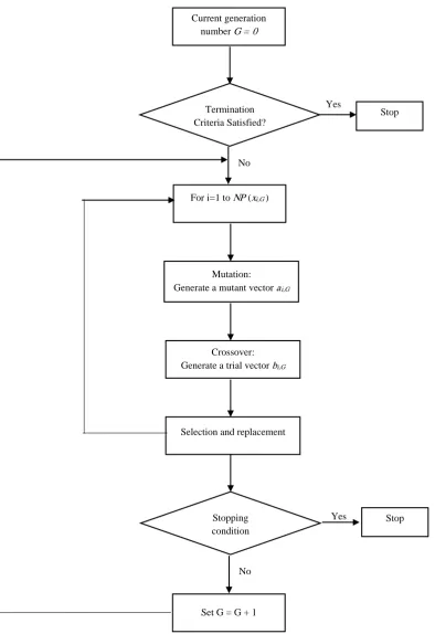
The DE algorithm is meta-heuristic (Storn & Pierce, 1995) and finds the optimal solutions using an efficient search process in the direction of optimistic variables; it can change wrong directions into correct directions. This feature means that DE has speed (Amiri & Barbin, 2015). There are four main types of DE: generation of initial population, mutation, crossover, and selection.

The opposition-based differential evolution (ODE) was proposed by Rahnamayan and Wang (2008) to produce better results from DE on the large scale. Wang et al. (2012) used an orthogonal genetic algorithm (Leung, 2001) and proposed DE through orthogonal crossover. Deng et al. (2015) combined ODE and the orthogonal genetic algorithm to develop DE and proposed a novel local search operation for large-scale optimization problems. The DE standard framework is shown in Fig. 1 (Wang et al., 2012).

Variables xi,G and ai,G are the target resultant and its mutant resultant, respectively; bi,G is the vector that

performs the crossover and inherits properties from xi,G. For selection and replacement, bi,G, is chosen if

it has a better objective function than xi,G. It is evident that this method cannot be used in RCSPS

Fig. 1. DE standard framework

3.1 Chromosome representation and objective function

The chromosomes designed in the first step were those used by Shahdrok and Kianfer (2007). The design of the first part of the chromosomes was based on the activity sequence proposed by Hartmann (2000). For MRCPSP problems, the chromosomes should consist of three parts (Arjmand & Najafi, 2015). A list of available resource capacities has been proposed for second part of the present approach for SMRCPSP as:

Selection and replacement Current generation

number G = 0

)

G i, x

(

NP

For i=1 to

Mutation:

i,G a

Generate a mutant vector

Crossover:

i,G b

Generate a trial vector

Set G = G + 1 Stopping condition

Yes _Stop

No No

Stop Yes

1 1

(( ,...,_oI _nI ) , ( I ,..., I)).

I = i i ₊ M M_ρ (9)

3.2. Chromosome generation

The chromosome activity list can be produced by permutation of n activities; however, it is possible that the precedence list constraint makes the activity sequence infeasible. Different methods have been proposed to remove infeasible solutions (Arjmand & Najafi, 2015). The repair approach implemented by Shahdrok and Kianfer (2007) changes infeasible solutions to feasible solutions and was applied here. To generate the second part, resource capacities I

K

M , (k =1,..., )ρ were created for each chromosome I as:

min max min

(0,1) ( )

I

k k k k

M =M +rand × M −M . (10)

The capacity list in the second part should be a feasible number; thus, M_kI should be a number that lies between the defined lower and upper bounds. The lower and upper bounds are described as:

1

n

k _ik

i

M m

=

=

∑

(11)

1,..., 1

x{ ( ) / , { }}

n

k ik i i n ik

i

M Ma m D T Max ₌ m

=

=

∑

× (12)

The repair operator was used to change infeasible solutions for the capacity list. For this operator, if the

jth value of M_jI of the chromosomes is outside search region [M_k ,M k], then M I_j is updated as:

min{ , 2 }

min{ , 2 }

I I

k _{k j j k}

I j

I I

k

k j k j

M M M if M M

M

M M M if M M

 _{− ≤} 

 

=  

 − ≤ 

 

(11)

In each generation, M k and M _k should be updated so that they equal the maximum values of the parameters in the current population.

3.3 Mutation

The lineament feature of DE is its mutation operator. An important difference between DE and other meta-heuristic algorithms is the precedence of mutation over crossover. For chromosome

1 1

(( ,..., ) , ( ,..., ))

p p p p p

o n

I = i i + M M_ρ , apply the DE mutation by selecting three random chromosomes from

population, Ia, Ib and Ic.For the activity sequence, create Inbas equal to Ib, but change the places that are

same as Ic to empty. This produces I_nb =(i_onb,...,i_nnb₊₁) ∃j j, ∈{0,...,n+1} _{in which} i_jnb is empty.

To fill the empty places of I_nb,i_jnb, insert i_jnb = i_la, where l is the lowest index such that

0 1

{ ,..., }

a nb nb

l n

i ∉ i i ₊ . For example, if n = 6, then (ioI,...,inI+₁)=(0,1, 2, 3, 4, 5, 6, 7). Three random

chromosomes are then chosen from the population, such as (Ia = (i_oI,...,i_nI₊₁)=(0,1, 3, 2, 5, 4, 6, 7), Ib =

1

(j_oI,...,j_nI₊ )=(0, 2, 3,1, 4, 5, 6, 7)

, and Ic = ( ,..., 1) (0,1, 6, 3, 4, 5, 2, 7)

I I

o n

i i ₊ = ) to produce

1

( nb,..., nb ) (0, 2, 3,1, , , 6, 7)

nb o n

I = i i ₊ =   . The new child is Inewchil =(i_oC,...,i_nC₊₁)=(0, 2, 3,1, 5, 4, 6, 7). Because it is possible for the result of the mutation to be infeasible, the repair approach is used to change an infeasible mutation to a feasible one.

Next, mutation operators were used for the second part of the list. Let M_K =(M₁p,...,M_ρp) be the

• DE/rand/1 mutation: For each resource i, a new solution is generated as:

, , ( , , )

newchil a b c

k i k i k i k i

M =M +F M −M (12)

where random indices a b and c, ∈{1,...,NP} are integer numbersand F is a real and constant factor which determines the consolidation of different variations of (M_{k i}b_, −M_{k i}c_, ) (Biju et at., 2015).

Higher diversity is created in the generated population for larger values of F and lower values for F

result in faster convergence (Rahnamayan & Wang, 2008).

• DE/rand/2 mutation: A new chromosome is generated from the mutation by randomly selecting

four chromosomes (Ic, Ib, Id, Ie) from the population.For each resource i, a new solution is generated

as:

, , ( , , ) ( , , )

newchil a b c d e

k i k i k i k i k i k i

M =M +F M −M +F M −M , (13)

where random indices a b c d and e, , , ∈{1,..., }n are integers that are mutually exclusive. F is a real and constant factor which determines the consolidation of different variations of

, , , ,

(M_{k i}b −M_{k i}c )and M( _{k i}d −M_{k i}e ). It is possible for the result of a mutation of the capacity to be infeasible; thus, the repair operator of the capacity list is used to change an infeasible solution to a feasible solution.

3.4 Crossover

DE employs the crossover operation to generate new solutions to increase diversity in the population. This operator is the same that for a crossover in a GA (Amiri & Barbin, 2015). Two crossover operators are applied in the DE method.

• Binomial crossover: Chromosome ICH =((M_oCH,...,M_nCH₊₁) , (M₁CH ,...,M_ρCH))is generated as:

(0,1) newchil

i i rand

CH

i _p

i

M if rand CR or i i

M

M otherwise

 ≤ =

 =  

(14)

where index i_rand is a random number in [1, n]. CRis the crossover constant∈(0,1]and is the user-defined crossover control parameter. Because i_rand is used, R_iCH is always different from M_ip(Wang et al., 2012).

• Exponential crossover: Chromosome ICH =((i_oCH,...,i_nCH₊₁) , (M₁CH ,...,MCH_ρ )) is generated as:

for , 1 ,..., 1

otherwise newchil

j _{n n n}

CH

i _p

j

i j z z z Z

i

i

 = + + −

 =  

(15)

where i = 1, 2,. . . , n , j = 1,2,. . . ,n and _n define the modulo function for modulus n. The index

z is a random number between 1 and n. Integer Z was chosen from [1, n] and has a probability of

1

( ) u , 0

r

p Z ≥u =CR − u > . Parameters z and Z are then regenerated for each chromosome ICH _{and the}

exponential crossover can be used for the capacity list. The first part of equation is the same for the activity sequence. To choose iCHIL_j from the second part, use ipsuch that ICH is

1 1 1

(i_oCH,...,iCH_j− , , i_iCH+ ,...,i_nCH+ ) and insert ifp, where f is the lowest index such that { 0 ,..., 1}

p CH CH

f n

It is better to use binomial crossover for the capacity list and exponential crossover for the schedule list. It is important after each crossover to apply the repair operator.

3.5 Selection

This operation decides whether ICH _{should become part of the next generation (}G + 1). For this purpose, it is compared with parent chromosome IP using greedy selection. Selection is done as follows:

, , ,

, 1

,

if ( ) ( ) otherwie.

CH CH P

i G i G i G

i G _P

i G

I f I f I

I

I

+

 < 

 

=  

 

 

(16)

where I_{i G, +1} is the selection chromosome for the next generation. These steps are repeated until a stopping criterion is met or the best solution is achieved. The best fitness values have, thus been obtained and the matrix of the best solution consisting of total overtime work, duration, and cost can be obtained (Biju et al., 2015).

3.6 Local search

The performance of DE depends on the dimensionality of the optimization problems. As the search space increases dimensionality, the cases increase the complexity of the problem exponentially. This increase in complexity can reduce performance; however, the performance of DE will increase quickly for problems with a large number of variables. Most problems have a large number of variables; thus, support of scalability is a valuable characteristic for any optimization method. A local search is proposed to address this issue. A number of studies have examined local search in DE. The opposition-based search proposed by Rahnamayan and Wang (2008) and orthogonal crossover proposed by Wang et al. (2012) were used here. Deng et al. (2015) combined these two operators and proposed a novel local search operation for large scale optimization problems.

3.6.1 Opposition-based DE

This operator was proposed by Rahnamayan and Wang (2008), who proposed quasi-opposition-based learning (ODE) and proved that isotropy speed and solution correctness of DE can be improved. A quasi-opposite point is more likely to be closer to the solution of the optimization problem than the quasi-opposite one (Deng et al., 2015). Opposition-based DE was carried out only for the capacity list. This operator works based on jumping rate Jr. ODE forces the process to jump to a new chromosome candidate that

may be better than the current one (Rahnamayan and Wang, 2008). This operation is applied after generating a new population by selection, crossover, and mutation. After calculating the opposite population (Np: number of population), the best chromosomes are selected from the union of the current

population and the opposite population. The opposite point of (M₁I ,...,M_ρI) for

1 1

(( ,..., ) , ( ,..., ))

p p p p p

o n

I = i i ₊ M M_ρ is defined by its components as:

p p p p

k k k k

OM =MinM +MaxM −M , (17)

where k ∈K ={1,..., }ρ , MaxR_kp is the maximum number of resources k in Np , and MinM_kp is the

minimum number of resources k in Np. In the first generation, MaxM_kp = M k and MinM_kp = M_k . Comprehensive experiments by Rahnamayan and Wang (2008) revealed that Jr should be a number in

[0, 0.4]. It is important after each local search repair to apply the operator.

3.6.2 Orthogonal crossover

orthogonal crossover. This combination improved the ability of orthogonal crossover. An orthogonal array for K factors with Q levels and M combinations can be denoted as (K), ( K)

M

L Q . For example,

4

9(3 )

L is used in DENSL as follows (Deng et al, 2015):

4 9

1 1 1 1

1 2 2 2

1 3 3 3

2 1 2 3

(3 ) 2 2 3 1

2 3 1 2

3 1 3 2

3 2 1 3

3 3 2 1

L

 

 

 

 

 

 

 

=

 

 

 

 

 

 

 

(18)

Zhang and Leung (1999) believed each trial solution in a search algorithm could be regarded as an experiment. Another version of OX was introduced by Leung and Wang (2001) which proposed a quantization technique for OX that was called QOX by Wang et al. (2012). QOX was employed in the present algorithm. Orthogonal crossover was used only for the capacity list to improve the search ability of DE. Note that it is not logical to apply QOX to every pair of mutant and target chromosomes because it would consume too much computing time; thus, for every generation, QOX was performed for only one member of the population (Wang et al., 2012).

Let chromosome Ip =((i_op,...,i_np₊₁) , (M₁p,...,M_ρp)) be a selection member for QOX. First, mutation and crossover operations are carried out as explained above. The capacity list is given two parent individuals

1

( ,..., )

P P P

K

M = M M_ρ and M_Knewchil =(M₁newchil,...,M_ρnewchil) where P K

M is the capacity list from the

parentand newchil K

M is the capacity list from the mutation operator. QOX first quantizes the search range

and defines Q levels li1, li2,…, liQ based onL_M(QK)) as follows:

,

1

min( , ) (max( , ) min( , )), 1,..., .

1

P newchil P newchil P newchil

i j i i i i i i

j

l M M M M M M j Q

Q −

= + • − =

−

(19)

Eq. (18) and Eq. (19) can generate nine children given two parents. A general explanation of QOX has been provided by Wang et al. (2012) After generating nine children, the activity sequence achieved from crossover and mutation is combined with the nine children. The evaluation unfitness function is carried out for these nine children and the best solution is chosen (Wang et al., 2012).

3.6.3 Novel local search operation

Deng et al. (2015) combined the orthogonal crossover and opposition operator to propose a new local search. This local search can generate 18 experimental chromosomes to locate more space. Because of the large number of chromosomes, this operation cannot be used for each pair of mutation chromosomes; thus, one individual is chosen from every population for a local search. This method is similar to orthogonal crossover except that, that after producing nine children using orthogonal crossover, it generates the opposite of each set of nine children. Next, the unfitness function is carried out on the 18 children and the best solution is chosen from among them.

4. Testing and Comparison of DE Algorithm

Herroelen (1992) to solve 690 problems. The proposed DE method was used on the single mode test cases in the PSPLIB library. Evaluation of the results requires determination of the initial parameters in meta-heuristic algorithms. The DE algorithm is susceptible to its input data, which has a major effect on DE performance. A flexible and efficient solution can be achieved using the appropriate parameters. One important parameter is the number of populations in the meta-heuristic algorithms. This problem suffers from immature convergence with a low population size and will not reach an eligible response that is approaches the global optimum. With a large population size, more time for computation can be expected. This means that determining the appropriate population size to achieve the optimal solution is important. Table 1 shows the parameters that most affect the performance of the proposed model (Amiri and Barbin, 2015).

Table 1

Performance parameters

Parameters Values

No.Population 100

CR 0.9

F 0.9

Selection Randomize

Jumping rate 0.3

Generation 1000, 5000, 50000

The j30 and j60 sets of problems were selected from the PSPLIB library. The algorithms were run through 10 iterations. All the results were calculated by using Matlab 2014. To analyze the effect of a scheduling scheme, the SSS and PSS scheduling schemes were considered. The DE/rand/1 and DE/rand/2 and their crossover, binomial crossover, and exponential crossover mutations were used. The opposition-based DE, orthogonal crossover, and novel local search operations were the local searches used.

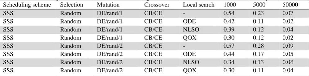
Table 2

Effect of schedule generation scheme, mutation operators, and selection method on average deviation

Scheduling scheme Selection Mutation Crossover Local search 1000 5000 50000

SSS Random DE/rand/1 CB/CE - 0.54 0.23 0.07

SSS Random DE/rand/1 CB/CE ODE 0.42 0.11 0.02

SSS Random DE/rand/1 CB/CE NLSO 0.39 0.12 0.04

SSS Random DE/rand/1 CB/CE QOX 0.30 0.12 0.02

SSS Random DE/rand/2 CB/CE - 0.57 0.28 0.09

SSS Random DE/rand/2 CB/CE ODE 0.44 0.17 0.05

SSS Random DE/rand/2 CB/CE NLSO 0.34 0.13 0.06

SSS Random DE/rand/2 CB/CE QOX 0.30 0.11 0.04

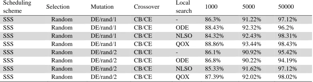
Table 3

Effect of schedule generation scheme, mutation operators, and selection method on average deviation Scheduling

scheme Selection Mutation Crossover

Local

search 1000 5000 50000

SSS Random DE/rand/1 CB/CE - 86.3% 91.22% 97.12%

SSS Random DE/rand/1 CB/CE ODE 88.43% 92.32% 96.2%

SSS Random DE/rand/1 CB/CE NLSO 84.32% 92.43% 98.31%

SSS Random DE/rand/1 CB/CE QOX 88.86% 93.44% 98.43%

SSS Random DE/rand/2 CB/CE - 86.1% 90.92% 95.42%

SSS Random DE/rand/2 CB/CE ODE 86.8% 90.22% 94.19%

SSS Random DE/rand/2 CB/CE NLSO 85.33% 91.62% 97.12%

SSS Random DE/rand/2 CB/CE QOX 87.39% 92.02% 98.02%

Over time, the algorithms performing the local search showed the best average percentage of deviation from the optimal solution rather. The results obtained using DE were compared with the results of a GA (Table 4). For each method, the minimum, maximum, and average results were obtained in 10 iterations. The standard deviation was also calculated.

Table 4

Comparison of performances of GA and DE

Name GA DE

Min Avg. Max SDev Min Avg. Max SDev

j301_1 512 512 512 0 512 512 512 0

j305_2 1214 1219.5 1246 11.2 1214 1214 1214 0

j3010_1 698 698 698 0 698 698 698 0

j3015_1 1054 1054 1054 0 1054 1054 1054 0

Average 869.5 870.8 877.5 2.8 869.5 869.5 869.5 0

j601_1 409 415 438 12.33 409 409 409 0

j605_1 1018 1096 1167 19.19 918 926.33 984.64 21.59

j6010_1 1281 1284 1291 2.43 1264 1266 1268 2.12

j6015_1 1480 1480 1480 0 1480 1480 1480 0

Average 1047 1068.75 1094 8.48 1017 1020.25 1035.41 5.92

Table 4 shows that the minimum, maximum, and average results achieved from DE are better than those obtained results from the GA. The average standard deviation for the j30 problems for the DE was 0, which is better than that for the GA (2.8). Table 4 also lists the results for the j60 problems. The increase in the size of the problems increased the standard deviation, but DE continued to obtain better results than GA. Table 5 shows the success rates for the j30, j60, and j120 problems for 1000 and 5000 schedule generations. Tables 4 and 5 demonstrate that DE performed better and produced more appropriate results than did GA. All answers prove that the DE algorithm performed well when solving RCSPS.

Table 5

Success rates for j30, j60, and j120

GA DE

Generations 1000 5000 1000 5000

j30 81.50% 91.30% 89.50% 94.67%

j60 74.23% 73.33% 79.32% 84.32%

j120 29.84% 34.45% 45.53% 52.67%

5. Conclusion

differently for different problems. Local searches were proposed to avoid being trapped in the local optima for large-scale optimization problems and to increase the ability of the algorithm to solve RCPSP problems. The effectiveness and speed of the proposed model was demonstrated by comparison with a sample project that was previously solved using GA. The proposed model solved the RCSPS with accurate convergence to optimal solutions, which was the main objective of this work. The results of DE have revealed that the proposed algorithms performed better than the genetic algorithms with less error. The DE algorithm will be proposed for different types of scheduling problems in the future.

Acknowledgements

This research was done by help of Amirhoseyn Khalili and Amin Sameti.

References

Akbari, R., Zeighami, V., & Ziarati, K. (2011). Artificial bee colony for resource constrained project scheduling problem. International Journal of Industrial Engineering Computations, 2(1), 45-60. Akpan, E. O. (1997). Optimum resource determination for project scheduling. Production Planning &

Control, 8(5), 462-468.

Amiri, M., & Barbin, J. P. (2015). New approach for solving software project scheduling problem using differential evolution algorithm.

Arjmand, M., & Najafi, A. A. (2015). Solving a multi-mode bi-objective resource investment problem using meta-heuristic algorithms. 1, 41-58.

Blazewicz, J., Lenstra, J. K., & Kan, A. R. (1983). Scheduling subject to resource constraints: classification and complexity. Discrete Applied Mathematics, 5(1), 11-24.

Bilolikar, V. S., Fr, C. R., & Jain, M. K. (2014). An adaptive crossover genetic algorithm for multi-mode resource constrained project scheduling with discounted cash flows. 1-9. Proceeding.

Biju, A. C., Victoire, T., & Mohanasundaram, K. (2015). An Improved Differential Evolution Solution for Software Project Scheduling Problem. The Scientific World Journal, Article ID 232193.

Hsu, C. C., & Kim, D. S. (2005). A new heuristic for the multi-mode resource investment

problem. Journal of the Operational Research Society, 56(4), 406-413.

Demeulemeester, E., & Herroelen, W. (1992). A branch-and-bound procedure for the multiple resource-constrained project scheduling problem. Management science, 38(12), 1803-1818.

Deng, C., Dong, X., Yang, Y., Tan, Y., & Tan, X. (2015). Differential Evolution with Novel Local Search

Operation for Large Scale Optimization Problems. In Advances in Swarm and Computational

Intelligence (pp. 317-325). Springer International Publishing.

Demeulemeester, E. (1995). Minimizing resource availability costs in time-limited project networks.

Management Science, 41(10), 1590-1598.

Drexl, A., & Kimms, A. (2001). Optimization guided lower and upper bounds for the resource investment problem. Journal of the Operational Research Society, 340-351.

Hartmann, S., & Kolisch, R. (2000). Experimental evaluation of state-of-the-art heuristics for the resource-constrained project scheduling problem. European Journal of Operational Research, 127(2), 394-407.

Jia, Q., & Seo, Y. (2013). Solving resource-constrained project scheduling problems: conceptual validation of FLP formulation and efficient permutation-based ABC computation. Computers & Operations Research, 40(8), 2037-2050.

Klimek, M. (2011, January). A genetic algorithm for the project scheduling with the resource constraints. In Annales UMCS, Informatica (Vol. 10, No. 1, pp. 117-130).

Kolisch, R. (1996). Serial and parallel resource-constrained project scheduling methods revisited: Theory and computation. European Journal of Operational Research, 90(2), 320-333.

Kolisch, R., & Hartmann, S. (2006). Experimental investigation of heuristics for resource-constrained project scheduling: An update. European journal of operational research, 174(1), 23-37.

Kolisch, R., & Padman, R. (2001). An integrated survey of deterministic project scheduling. Omega,

29(3), 249-272.

Koulinas, G., Kotsikas, L., & Anagnostopoulos, K. (2014). A particle swarm optimization based hyper-heuristic algorithm for the classic resource constrained project scheduling problem. Information Sciences, 277, 680-693.

Leung, Y. W., & Wang, Y. (2001). An orthogonal genetic algorithm with quantization for global numerical optimization. Evolutionary Computation, IEEE Transactions on, 5(1), 41-53.

Merkle, D., Middendorf, M., & Schmeck, H. (2002). Ant colony optimization for resource-constrained project scheduling. Evolutionary Computation, IEEE Transactions on, 6(4), 333-346.

Möhring, R. H. (1984). Minimizing costs of resource requirements in project networks subject to a fixed completion time. Operations Research, 32(1), 89-120.

Najafi, A. A., & Niaki, S. T. A. (2006). A genetic algorithm for resource investment problem with discounted cash flows. Applied Mathematics and Computation, 183(2), 1057-1070.

Nübel, H. (1999). A branch and bound procedure for the resource investment problem subject to

temporal constraints. Inst. für Wirtschaftstheorie und Operations-Research.

Nübel, H. (2001). The resource renting problem subject to temporal constraints. OR-Spektrum, 23(3), 359-381.

Rahmani, N., Zeighami, V., & Akbari, R. (2015). A study on the performance of differential search algorithm for single mode resource constrained project scheduling problem. Decision Science Letters,

4(4), 537-550.

Rahnamayan, S., Tizhoosh, H. R., & Salama, M. M. (2008). Opposition versus randomness in soft computing techniques. Applied Soft Computing, 8(2), 906-918.

Storn, R., & Price, K. V. (1996, May). Minimizing the Real Functions of the ICEC'96 Contest by

Differential Evolution. In International Conference on Evolutionary Computation (pp. 842-844).

Shadrokh, S., & Kianfar, F. (2007). A genetic algorithm for resource investment project scheduling problem, tardiness permitted with penalty. European Journal of Operational Research, 181(1), 86-101.

Wang, H., Rahnamayan, S., & Wu, Z. (2013). Parallel differential evolution with self-adapting control parameters and generalized opposition-based learning for solving high-dimensional optimization problems. Journal of Parallel and Distributed Computing, 73(1), 62-73.

Wang, Y., Cai, Z., & Zhang, Q. (2012). Enhancing the search ability of differential evolution through orthogonal crossover. Information Sciences, 185(1), 153-177.

Xiao, L., Tian, J., & Liu, Z. (2014, June). An Activity-List based Nested Partitions algorithm for Resource-Constrained Project Scheduling. In Intelligent Control and Automation (WCICA), 2014 11th World Congress on (pp. 3450-3454). IEEE.

Yang, B., Geunes, J., & O’brien, W. J. (2001). Resource-constrained project scheduling: Past work and new directions. Department of Industrial and Systems Engineering, University of Florida, Tech. Rep. Zhang, Q., & Leung, Y. W. (1999). An orthogonal genetic algorithm for multimedia multicast routing.

Evolutionary Computation, IEEE Transactions on, 3(1), 53-62.

Ziarati, K., Akbari, R., & Zeighami, V. (2011). On the performance of bee algorithms for resource-constrained project scheduling problem. Applied Soft Computing, 11(4), 3720-3733.

Zimmermann, J., & Engelhardt, H. (1998). Lower bounds and exact algorithms for resource leveling