Buffer clustering policy for sequential production lines with deterministic processing times Pages 555-572 Download PDF

(1)

* Corresponding author. Tel: +1 (224) 715-6799 E-mail: [email protected] (F. Schuler)

International Journal of Industrial Engineering Computations 7 (2016) 555–572

Contents lists available at GrowingScience

International Journal of Industrial Engineering Computations

homepage: www.GrowingScience.com/ijiec

Buffer clustering policy for sequential production lines with deterministic processing

times

Francesca Schuler*_{and Houshang Darabi}

Mechanical and Industrial Engineering, University of Illinois, Chicago, USA

C H R O N I C L E A B S T R A C T

Article history: Received April 4 2016 Received in Revised Format April 27 2016

Accepted May 6 2016 Available online May 6 2016

A sequential production line is defined as a set of sequential operations within a factory or distribution center whereby entities undergo one or more processes to produce a final product. Sequential production lines may gain efficiencies such as increased throughput or reduced work in progress by utilizing specific configurations while maintaining the chronological order of operations. One problem identified by the authors via a case study is that, some of the configurations, such as work cell or U-shaped production lines that have groups of buffers, often increase the space utilization. Therefore, many facilities do not take advantage of the configuration efficiencies that a work cell or U-shaped production line provide. To solve this problem, the authors introduce the concept of a buffer cluster. The production line implemented with one or more buffer clusters maintains the throughput of the line, identical to that with dedicated buffers, but with the clusters reduces the buffer storage space. The paper derives a time based parametric model that determines the sizing of the buffer cluster, provides a reduced time space for which to search for the buffer cluster sizing, and determines an optimal buffer clustering policy that can be applied to any N-server, N+1-buffer sequential line configuration with deterministic processing time. This solution reduces the buffer storage space utilized while ensuring no overflows or underflows occur in the buffer. Furthermore, the paper demonstrates how the buffer clustering policy serves as an input into a facility layout tool that provides the optimal production line layout.

Keywords:

Sequential Production Buffer Cluster Deterministic Configuration

1. Introduction

(2)

configuration in Fig. 2 called a hybrid serial-work cell configuration to gain increased throughput. As a result of this change, the facility encountered a production floor space utilization problem. In these figures, the squares without a grid pattern represent server stations where a process step occurs. The squares with a grid pattern represent buffers. The stations may be manual, semi-automated, or fully automated. The groups of buffers in Fig. 2 may vary in the number of buffers within the work cell and the number of serial stations in between the work cells as shown.

Fig. 1. N-server, N+1 buffer serial line

Fig. 2. Variable station work cells with one or more serial stations in between

In this scenario, because the buffers were sized separately (i.e. dedicated buffers) with respect to the serial line and grouped in the center of the work cell, the grouped buffers were not leveraging available space in the neighboring buffers during the production shift. Therefore, the work cell exceeded the typical space of the production line. The authors proposed transitioning the grouped buffers in the center of the work cell to a single buffer cluster shown in Fig. 3 which enables increased buffer utilization and reduces the size of the grouped buffers, reducing the buffer storage space. This allows the facility to benefit from efficiencies (e.g., increased throughput, work in progress reduction) by use of alternate configurations. In addition, discussed in the case study in section 4 is how sensitivity analysis of the buffer cluster size can be conducted using the models derived herein varying parameters such as the production demand and process times.

Fig. 3. Variable station work cells with serial stations in between using buffer cluster concept

(3)

F. Schuler and H. Darabi

Once the buffer clustering policy is identified for a production line, an activity relationship chart is created for the buffers and stations in the production line and the amount of space assigned to each activity is determined. From the space relationship diagram, one or more feasible layout concepts are generated. The optimal production line layout is then selected.

This paper proceeds with a literature review in the second section. The third section describes the problem formulation and derives the model that is used to solve the size of the buffer cluster for any N-server, N+1-buffer, sequential line. An optimization framework is derived that enables a buffer clustering policy and provides an output of the buffer sizing for that policy that ensures no buffer overflows. In the fourth section, the authors apply the model to the case study and review the results. The final section discusses the conclusions.

2. Literature review

Given the industry example discussed in the introduction, how the research at hand differs from the prior art is assessed. Quantitative analysis of production lines includes the line balancing problem (Becker & Scholl, 2006), the buffer allocation problem (Charharsooghi & Nahavandi, 2003), queuing network performance and blocking (Govil & Fu, 1999; Li et al., 2009). Literature also discusses these concepts explored with the addition of flexible manufacturing systems with varying configurations (serial, sequential, work-cells) and product types (Senanayake & Subramaniam, 2013; So, 1989).

The line balancing problem includes the positioning and sizing of the buffers and the overall throughput resulting in the buffer allocation problem. Wei et al. (1989) estimate stochastically via optimization the buffer size in a serial manufacturing system. Chaharsooghi and Nahavandi (2003) present a heuristic algorithm to find the optimal allocation of buffers that maximizes throughput. Yamashita and Altiok (1998) implement a dynamic programming algorithm that uses decomposition to minimize buffer allocation but still meeting target throughput in production lines with phase-type processing times. There are several buffer allocation strategies: (1) Equal Buffer allocates buffers equally over the line, (2) Chow’s Rule (Chow, 1987) uses dynamic programming to solve the buffer allocation problem with a fixed total buffer size, (3) L&L’s Rule (Liu & Lin (1994)), uses a different set of equations than Chow to estimate the throughput and (4) C&N’s rule (Chan & Ng (2002)) where all possible allocations of buffers are tried and then the allocation with the highest estimated throughput is selected. Gershwin and Schor (1999) minimize the total buffer space using a production rate constraint while maximizing production rate using a total buffer space constraint. Enginarlar et al. (2000) ensure the smallest level of buffering with the desired production rate in serial lines with unreliable machines. Enginarlar et al. (2002) also introduces the concept of Lean Level of Buffering where buffer capacity is normalized and production line efficiency is achieved using exact methods for three machine lines and estimation methods for lines with more than three machines.

Queuing network performance literature includes quantitative analysis for production systems and considers production rates, average buffer levels and probabilities of blockage (Govil & Fu, 1999; Li et al., 2009). Gershwin (1987) developed a method using conservation of flow for evaluation of performance measures for lines with finite buffers. Lim et al. (1990) developed an aggregation method that converges on a production rate eliminating the need for simulations. Kouikoglou and Phillis (1991, 1994 and 1995) use a probabilistic technique that observes a limited number of events which are sufficient to determine the system performance and average buffer sizes. Morrison (2010) demonstrates that flow line models with deterministic service times using recursion to calculate the overall delay of entities in the system.

(4)

investigate the utilization of work-cell and reconfigurable manufacturing systems to increase the efficiency and capacity of production lines. Ichikawa’s study (2009), for example, investigates a laptop production system and optimizing the supply of parts via material handlers from the receiving area to the cells. Another study (Aghazadeh et al., 2011) analyzes use of product-oriented layout, material handling and layout of work-cells to maximize production efficiency in areas such as average units produced per day, labor cost per unit and distance traveled to procure parts. Logendran and Karim (2003) uses a non-linear programming model consisting of binary and integer variables and a tabu search type algorithm to determine the availability of alternative locations for a work-cell and the use of alternative routes to move part loads between cells when capacity is limited. Youssef and ElMaraghy (2007) introduce a configuration selection approach that minimizes reconfiguration effort but still supports the capacity needs of production. Matta et al. (2005) use discrete event simulation and graph theory to demonstrate that technological devices moving entities from a machine to a single common buffer area of the system can improve production rates.

This paper differs from the prior literature reviewed in that it presents methods for extracting the buffer size where the buffer space is shared by several stations (via a buffer cluster) using methods derived from state space parameters with respect to time for any sequential N-server, N+1-buffer production line. The buffer sizing model is then utilized in an optimization framework that enables setting of the policy specifying the buffers that can be clustered ensuring no buffer overflows. The model provides an output of the required buffer cluster sizing for that policy and allows the facility to set the policy that minimizes space utilization of the production line.

3. Buffer cluster model

The buffer cluster model is presented in two parts. The first part (section 3.1) is the problem formulation where no clustering is assumed. This provides the model ultimately used for sizing the buffer cluster for any N-server, N+1-buffer sequential production line. In the second part (section 3.2), the model in section 3.1 is extended to a buffer cluster. Section 3.2 derives the optimization framework that determines the buffer cluster sizing required and enables a buffer clustering policy.

3.1. Buffer sizing problem formulation

In this section, the parameters used for deriving the formulation ultimately used for sizing the buffer cluster in any N-server, N+1-buffer sequential production line are defined. The number of arrivals and departures at Server Si,i = 1, 2…N by any given timet are calculated. Next the number of arrivals and

departures from any buffer Bi, i = 1, 2,…N+1by any given time t are derived. The relationships are

generated to derive the maximum number of entities (parts) a buffer will experience and the number of entities at any given time t, Bi(t). Bi(t) is then extended in section 3.2 to determine the buffer cluster size.

Before deriving the aforementioned relationships, the notations, assumptions and definitions are listed.

Notations:

N1) K1 = Magnitude of inventory at B1at time t=0, K1 = 1, 2,…N (Constant).

N2) BAi(t) = Cumulative number of arrivals at buffer Bi by time t, i=1,2,…N+1.

N3) BDi(t) = Cumulative number of departures from buffer Bi by time t, i=1,2,…N+1.

N4) SAi(t) = Cumulative number of arrivals at server Si by time t, i=1,2,…N.

N5) SDi(t) = Cumulative number of departures from server Si by time t, i=1,2,…N.

N6) Ti, i = 1…N is the service time for server Si, i = 1…N (This includes both the process time of the

(5)

Assumptions:

A1) Each Server Si can process at most one entity at a time (capacity = 1).

A2) Each buffer Bi, i = 1…N+1, has a capacity greater or equal to the starting inventory.

A3) Service time Ti for each server Si is deterministic.

A4) At t=0-_{K1 is located in buffer}_B

1and all other buffers are empty.

A5) At time t = 0, B1 has a departure and S1 has an arrival.

A6) Buffer B1 has only departures while Buffer BN+1has only arrivals and every buffer Biin between has

both departures and arrivals; BA1(t) = 0; BDN+1(t) = 0 as shown in Fig. 1.

A7) If there is at least one part in Bi and Si is idle, then with no delay, an entity (part) is moved to Si for

processing.

A8) Machines are reliable.

Definitions:

D1) MTi = max[T1,T2…Ti ], i=1,2,…N.

D2) τi=∑ij=1Tj , i=1,2...N, and 0.

D3) MBi = Maximum number of entities that buffer Bi, i = 2,..,N will experience.

D4)

_{ }

is a floor function that maps a real number to the largest previous integer value. D5) It is trivial to see that the frequency of arrivals to server Si is 1

MT_i.

A framework utilizing deterministic process times is used as in practice data is not available to determine the correct process time probability distributions. In addition, probabilistic models do not allow production line managers to keep a pulse of the production line by knowing the status of each buffer or station at any given time. This framework enables sensitivity analysis by varying process times for one or more stations which will be shown in the case study (section 4).

This model supports adding inventory (that could be in the form of batches of varying sizes) anytime before the last item in inventory B1 leaves the first server S1 (i.e. a batch can be added anytime before t

= τ K1 1 ∗ MT). K1 can be either the initial inventory or a summation of inventory (in the

form of batches) throughout the shift.

The number of arrivals and departures from server Siare now calculated.

Theorem 1: For the sequential system the cumulative arrivals and cumulative departures at server Siat

time t is:

SAi t = min K1,1+

t - τi-1

MTi if t ≥τi-1

0 Otherwise

(1)

SDi t = min K1,1+

t - τi

MTi if t ≥τi

0 Otherwise

(2)

Proof: First, Eq. (1) holds for i=1 is shown. At i=1, τ1=∑j=1i Tj=T₁=MT1. 0. Based on the

sequential line assumption, at time t = 0, one part is loaded to server S1 (recall that K1 > 1). This part is

processed for units of time and if buffer B1 still carries a part, server S1 is loaded again. This

loading operation (arrival event) happens at time t= τ1. Continuing with this pattern, one can see that

server S1 is loaded at time stamp 0, τ₁, 2τ₁,…, K1τ

1, therefore the last loading of server S1happens at

time t=K1τ1. After this time no loading occurs as all the parts in buffer B1 have been depleted, and the

total number of arrivals to S1remains K1. This means that the cumulative number of arrivals to server S1

at time t can be shown by:

SA1 t = t

+1 0 ≤ t < 1

(6)

and it can immediately be concluded that SA1 t = min K1, 1+ t

τ1 , t ≥ 0.

This proves that Eq. (1) holds for i=1. Second, Eq. (1) is proven to hold for Si where 1 < i < N. By

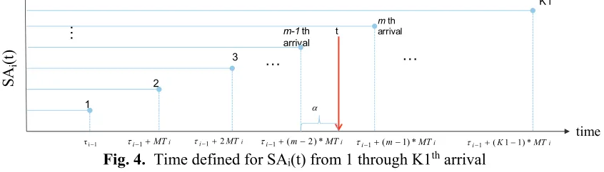
definition for t < , SAi(t) = 0 and for t = , SAi(t) = 1. Fig. 4 is based on the result of definition

D5. It shows that the cumulative arrivals to server Si at any time t. The interarrival times are MTi. The

case where 1< SAi (t) < K1 is now considered.

Fig. 4. Time defined for SAi(t) from 1 through K1th arrival

Assume that τi-1 + (m - 2)*MTi < t < _i_₁ + (m - 1)*MTi where m – 1 is an integer number and is the

number of arrivals before t. From the relationship that the frequency of arrivals to Server Si is 1

MTiand

that for the m – 1th and mth arrivals, time is defined in the following interval: τi-1 + (m – 2)*MTi < t < 1

i

 + (m – 1)*MTi,

t is defined as:

t = τi-1 + (m – 2)*MTi + α*MTi where 0 < α < 1

t - τi-1 = ((m – 2) + α)*MTi

When α = 1, the coefficient ((m – 2) + α) = m – 1= and Si experiences the mth arrival. For 0 <

α < 1, the coefficient = (m – 2) + α = m – 2 = t - τi-1

MT_i and Si has experienced the m-1th arrival.

Therefore, for 1 < SAi(t) < K1, SAi(t) = 1 + t - _MTτi-1

i . Based on the definition of arrival and departure of entities from server S1one can see that because of the relationship

SDi(t) = SAi(t + Ti) (3)

that means Eq. (2) holds. ■

Corollary 1: For the sequential system described in Fig. 1 the cumulative arrivals and cumulative

departures at buffer Bi at time t are:

BAi t min K1,1

t - τ_i-1

MT_i‐1 if t τi‐1

0 Otherwise

(4)

BDi t = min K1,1+

t - τi-1

MTi if t ≥τi-1

0 Otherwise

(5)

Proof: For any Bi where i = 2, 3…N+1, the number of arrivals at Biis equal to the number of departures

from Si-1 at a given time t. Therefore taking Eq. (2) from the perspective of Si-1 and applying the condition

from Eq. (6) proves Eq. (4).

BAi(t) = SDi-1(t) (6)

The number of departures from Biis equal to the number of arrivals at server Si. Therefore, taking Eq.

(1) from the perspective of arrivals at Si and applying the condition from Eq. (7) proves Eq. (5).

time

SA

i

(t

)

1 i

τ i1MTi i12MTi

1

2

3

i i1(K11)*MT



K1

m th arrival

…

i i1(m1)*MT



t

m-1 th arrival …

i i1(m2)*MT



(7)

BDi(t) = SAi(t) ■ (7)

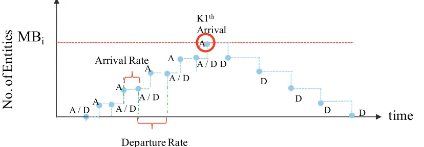
Corollary 2: For the sequential system, the maximum number of entities that buffer Bi will experience

given starting inventory K1 as shown in Fig. 5 is:

MBi = (K1 –1) - Y*(K1-1) (8)

Where Yi = MTi-1

MTi for i = 2…N.

When Ti > MTi-1, then MTi-1 < MTi and Yi < 1. When Ti < MTi-1, then MTi = MTi-1 and Yi =1.

This is proven for MBi, i = 2,3,…N and when Yi < 1.

When Yi =1, MBi = 0, thus a buffer size = 1 is required for transport only to the next process. This is

called a transport buffer and MBi = 1 is assigned.

Fig. 5. Maximum number of entities that buffer Bi will experience given inventory K1

For Bi of interest, at any given time t the number of entitiesis equal to:

Bi(t) = BAi(t) - BDi(t), Bi(t) > 0 (9)

The time (say T) when Bi(t) reaches its maximum level is derived and then entered into Eq. (9), therefore

calculating MBi. By assumption, the first departure from Si-1 and the first arrival to Si happen

simultaneously. After this event, because MTi = Ti > MTi-1 and using the relationship that the frequency

of arrivals to Server Si is 1

MT_i, the departure rate from Si-1will be greater than the arrival rate to Si. This

causes the accumulation in Bi to increase until the last departure (K1th departure) from Si-1occurs.

Therefore the maximum accumulation happens when the last departure from Si-1occurs.

T = MTi-1*(K1-1) + τi-1 (10)

Plugging in T from Eq. (10) into Eq. (11) and using the results of Corollary 1:

Bi(t) = BAi(t) - BDi(t) = min (K1, 1+ t - _MTτi-1

i-1 ) – min (K1, 1 +

t - τi-1

MTi )

(11)

= MBi = MTi-1*(K1-1)

MTi-1

MT_i-1*(K1-1)

MTi = (K1 –1) - Y*(K1-1) ■

3.2. Optimization framework formulation for buffer clustering policy

In this part, the buffer clustering optimization framework is derived utilizing the model from section 3.1 to provide the buffer cluster sizing and an optimal buffer clustering policy. Before deriving the

No

. o

f E

nt

it

ie

s

_MB

i

time

Departure Rate Arrival Rate

K1th Arrival

A / DA

D

D _D

A

A A

A

A / D A / D

(8)

aforementioned relationships, the notations, assumptions and definitions are listed. Fig. 6 which shows the inventory profile in buffer Bi is used to illustrate the new notations K2i, K3i, t_1Bi̅ , t̅_2Bi and MBi -1.

Fig. 6. Illustration of K2i, K3i, t̅1Bi, t̅2Bi and MBi -1

Notations:

N7) Wjis a set of one or more buffers referred to as a buffer cluster.

N8) BBj is the maximum number of entities a buffer cluster Wj must be able to hold to ensure that no

overflows or underflows occur in the buffer cluster.

N9) Xj is a binary variable {0,1} and defines whether cluster Wj must be realized {1} or not {0} ( i.e. Xj

= 1 determines that cluster Wjmust be selected as a part of the buffer cluster policy).

N10) K2i is the last arrival to buffer Bi that occurs when the number of entities in buffer Bi is MBi - 1

N11) K3i is the number of entities that depart from buffer Bi changing the number of entities in buffer Bi

to MBi -1from MBi. This occurs right after the last arrival (K1 arrival) to buffer Bi.

N12) t̅ is the time of the first arrival changing the number of entities in buffer Bito MBi from MBi -

1(K2i + 1 arrival).

N13) t̅ is the time of the first departure (K3i) departing after the last arrival (K1 arrival) for buffer Bi.

It is the last time the number of entities in buffer Biequals MBi.

N14) q is the time the last entity departs from server SN to buffer BN+1

N15) H is the size each entity occupies within a cell of a buffer in square meters N16) G is the maximum size of a buffer cluster Wjin square meters

Assumptions: (Assumptions A1 through A8 from part A hold)

A9) Possible combinations (clusters) of buffers are given.

A10) A buffer Bimust be either a dedicated buffer or in a single cluster; thus, if {2, 3, …,i,…,N} denotes

the index set of intermediate buffers Bi and {1, 2, …j, …, C} the index set of buffer clusters Wj, then

Wj={2,3,…,N}

C

j=1

Although a buffer cluster must maintain the sequence of operations, meaning it must facilitate an entity to move in the sequence of operations from servers S1, S2, S3… to SN the buffers included in a cluster

should not necessarily be sequential. Therefore, a buffer cluster may include non-sequential buffers and still maintain the sequence of operations. The example in Fig. 7 shows non-sequential buffers B2 and B5

clustered (W1) and sequential buffers B3and B4 clustered (W2) while still maintaining the sequence of

operations S1 through S5 as shown by the arrows.

N

o.

o

f E

nti

ti

es MB

i

time

K1 Arrival

A / D A

D

D _D

A

A A

A / D A / D

A / D

MB

_i

-1

K2iArrival K3i Departure

A / D

t_2Bi t_1Bi

(9)

Fig. 7. Non-sequential and sequential buffer clusters maintaining sequence of operations

Eq. (8) in section 3.1 provides us with the maximum number of entities that buffer Biwill experience

over a given demand K1 within a production shift and is used for sizing the dedicated buffers to ensure that no overflows or underflows occur. The size required for the buffer cluster combinations is needed at any given time. Thus, for the buffer cluster, the buffer sizes leveraging Eq. (11) are assessed at every given time t as shown in Eq. (12) from the time of first arrival (τ1 of an entity in buffer B2 to the

completion of the production shift (q) (See assumption A6).

Bi t =min (K1, 1+ t - τ_i-1

MTi-1 ) – min K1, 1 -

t - τ_i-1

MTi ∀ t ∈[τi-1,q]

(12)

From Eq. (12) the search for the buffer cluster size requires a calculation at each time step throughout the production shift for every buffer Bi. This results in a significant number of computations. Appendix

B quantifies how the number of calculations can be substantially reduced. Before quantifying the savings, the authors solve for BBj. To solve for BBj, first solve for ̅ and ̅ (see Fig. 6) and then

prove that the maximum buffer cluster size required occurs when one of the individual buffers Bi is at a

maximum during the time interval ∈ ̅ , ̅ . To solve for ̅ , first solve for the last arrival (K2i) that occurs at MBi - 1. Eq. (8) is modified as shown in Eq. (13).

MBi -1 = (K2i –1) - Y*(K2i-1) (13)

Then to get the first arrival that occurs at MBi, solve for the time ̅ that the K2i + 1 arrival arrives to

buffer Bi

t̅1Bi = τi-1+ (K2i+1)-1 *MTi-1 (14)

To determine ̅ , first solve for the time of the K1th arrival to buffer Bi using Eq. (10) anduse Eq. (5)

to calculate the number of departures that have occurred by the K1th arrival. Then add one to the departures (named K3i) and calculate the time of this departure ( ̅ using Eq. (15).

t̅2Bi = τi-1+ K3i-1 *MTi (15)

The minimum size for a cluster Wj such that no overflows occur is shown in Eq. (16).

BBj = max

t ϵ∪_i=1N _[t_̅ 1Bi, t2 Bi̅ ]

∑Brϵ Wj Br(t) ∀ Wj (16)

In Appendix A, the authors prove that the buffer cluster size required occurs when at least one of the individual buffers in the cluster Wj is at a maximum according to Eq. (16). Thus the buffer cluster size

(10)

a buffer is at a maximum. This results in significant computational savings. The computational savings are calculated for the case study discussed in Section 4 and shown in Appendix B.

For a given production line, there can be hundreds of buffer cluster combinations. Consider a collection of candidate buffer clusters Wj, j  1, …, C, not necessarily disjoint, for which the minimum storage

requirements BBj have been computed via Eq. (16). Integer programming is used to find the buffer cluster

combination that provides the minimum total space occupied by all clusters. From here set the objective function as shown in Eq. (17) to determine the buffer cluster(s) size across the production line where Xj {0, 1} is a decision variable that determines whether the buffer cluster Wj should be realized or not.

As defined earlier each buffer can only participate in one and only one realized buffer cluster. The first set of constraints Eq. (18) show that a buffer Bi can only participate in one combination buffer cluster.

The second set of constraints Eq. (19) is the maximum size of a buffer cluster in square meters. The third set of constraints Eq. (20) is the binary constraints for Xj. Vj is defined to ensure constraint Eq. (18)

applies only to buffers within cluster Wj.

Vj = { i, Bi Wj } 1 < j < C

Objective Function:

min ∑Cj=1BBjX_j (17)

subject to:





 j V i j

j

X

:

1, 1 < i < N (18)

BBj*H*X_j < G, 1 < j < C (19)

= 0 or 1 ∀ j (20)

4. Applying model to the industry example

As discussed in the Introduction, the underlying motivation for this research was a case study where a manufacturing facility that produces mobile devices wished to change over from a serial line to a buffer cluster configuration. Table 1 shows the server stations and process times. The footprint for buffer cell holding an entity is 0.005m2_{. The maximum buffer cluster size is 1.825 m}2_.

Table 1

Production line processes

Element S₁ S₂ S₃ S₄ S₅ S₆ S₇

Process Times (Seconds) ₁ ₂ ₄ ₅ ₁₄ ₁₀ ₁₉

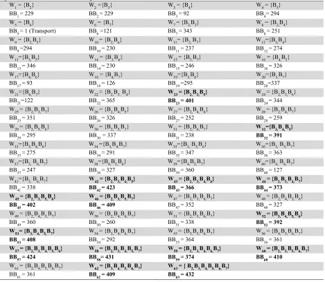
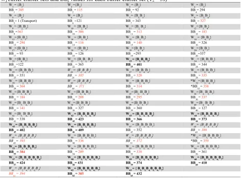
Given B1 and B8are the starting and ending inventory buffers, these are not included in the analysis. Eq.

(8) and Eq. (16) are used to populate Table 2 with Wj cluster sets and size for buffers B2 through B7. The

production line shift is 8 hours and 458 units are projected to ship by the end of the shift. There is a space constraint of 1.825 square meters for the buffer cluster size. In Table 2, the cells with bold text indicate that the cluster does not meet the space constraint (i.e. the buffer cluster size BBj > 365 entities).

(11)

Table 2

Wj Buffer cluster sets and BBj values for each buffer cluster set

W₁ = {B₂} W₂ ={B₃} W₃ = {B₄} W₄ = {B₅}

BB₁= 229 BB₂= 229 BB₃= 92 BB₄= 294

W₅ = {B₆} W₆ = {B₇} W₇= {B_2,B₃} W₈ = {B_2,B₄}

BB₅= 1 (Transport) BB₆ =121 BB₇= 343 BB₈= 251

W₉ = {B_2,B₅} W₁₀= {B_2,B₆} W₁₁= {B_2,B₇} W₁₂={B_3,B₄}

BB₉=294 BB₁₀= 230 BB₁₁= 237 BB₁₂= 274

W₁₃={B_3,B₅} W₁₄ = {B_3,B₆} W₁₅= {B_3,B₇} W₁₆ = {B_4,B₅}

BB₁₃= 346 BB₁₄= 230 BB₁₅= 246 BB₁₆= 326

W₁₇={B_4,B₆} W₁₈ = {B_4,B₇} W₁₉={B_5,B₆} W₂₀={B_5,B₇}

BB₁₇= 93 BB₁₈= 126 BB₁₉=295 BB₂₀=337

W₂₁={B_6,B₇} W₂₂= {B_2,B_3, B₄} W₂₃= {B_2,B_3,B₅} W₂₄= {B_2,B_3,B₆}

BB₂₁=122 BB₂₂= 365 BB₂₃= 401 BB₂₄= 344

W₂₅= {B_2,B_3,B₇} W₂₆= {B_2,B_4,B₅} W₂₇= {B_2,B_4,B₆} W₂₈= {B_2,B_4,B₇}

BB₂₅= 351 BB₂₆= 326 BB₂₇= 252 BB₂₈= 259

W₂₉= {B_2,B_5,B₆} W₃₀= {B_2,B_5,B₇} W₃₁= {B_2,B_6,B₇} W₃₂={B_3,B_4,B₅}

BB₂₉= 295 BB₃₀= 337 BB₃₁= 238 BB₃₂= 391

W₃₃={B_3,B_4,B₆} W₃₄={B_3,B_4,B₇} W₃₅={B_3, B_5,B₆} W₃₆={B_3, B_5,B₇}

BB₃₃= 275 BB₃₄= 291 BB₃₅= 347 BB₃₆= 363

W₃₇={B_3, B_6,B₇} W₃₈={B_4,B_5,B₆} W₃₉={B_4,B_5,B₇} W₄₀={B_4, B_6,B₇}

BB₃₇= 247 BB₃₈= 327 BB₃₉= 360 BB₄₀= 127

W₄₁={B_5, B_6,B₇} W₄₂= {B_2,B_3,B_4,B₅} W₄₃= {B_2,B_3,B_4,B₆} W₄₄= {B_2,B_3,B_4,B₇}

BB₄₁= 338 BB₄₂= 423 BB₄₃= 366 BB₄₄= 373

W₄₅= {B_2,B_3,B_5,B₆} W₄₆= {B_2,B_3,B_5,B₇} W₄₇= {B_2,B_3,B_6,B₇} W₄₈= {B_2,B_4,B_5,B₆}

BB₄₅= 402 BB₄₆= 409 BB₄₇= 352 BB₄₈= 327

W₄₉= {B_2,B_4,B_5,B₇} W₅₀= {B_2,B_4,B_6,B₇} W₅₁= {B_2,B_5,B_6,B₇} W₅₂= {B_3,B_4,B_5,B₆}

BB₄₉= 360 BB₅₀= 260 BB₅₁= 338 BB₅₂= 392

W₅₃= {B_3,B_4,B_5,B₇} W₅₄= {B_3,B_4,B_6,B₇} W₅₅= {B_3,B_5,B_6,B₇} W₅₆= {B_4,B_5,B_6,B₇}

BB₅₃= 408 BB₅₄= 292 BB₅₅= 364 BB₅₆= 361

W₅₇= {B_2,B_3,B_4,B_5,B₆} W₅₈= {B_2,B_3,B_4,B_5,B₇} W₅₉= {B_2,B_3,B_4,B_6,B₇} W₆₀= {B_2,B_3,B_5,B_6,B₇}

BB₅₇= 424 BB₅₈= 431 BB₅₉= 374 BB₆₀= 410

W₆₁= {B_2,B_4,B_5,B_6,B₇} W₆₂= {B_3,B_4,B_5,B_6,B₇} W₆₃= { B_2,B_3,B_4,B_5,B_6,B₇}

BB₆₁= 361 BB₆₂= 409 BB₆₃= 432

Objective Function

min ∑63i=1BBj*Xj

subject to:

Constraint for B2:

X1+X7+X8+X9+X10+X11+X22+X23+X24+X25+X26+X27+X28+X29+X30+X31+X42+X43

+X44+ X45 +X46+ X47+X48+X49+X50+X51+X57+X58+X59+X60+X61+X63=1 Constraint for B3:

X2+X7+X12+X13+X14+X15+X22+X23+X24+X25+X32+X33+X34+X35+X36+X37+X42+ X43 + X44+X45+X46+X47+X52+X53+X54+X55+X57+X58+X59+X60+X62+X63=1

Constraint for B4:

(12)

X4+X9+X13+X16+X19+X20+X23+X26+X29+X30+X32+X35+X36+X38+X39+X41+X42+ X45+X46+X48+X49+X51+X52+X53+X55+X56+X57+X58+X60+X61+X62+X63=1

Space Constraints BBj*0.005*Xj≤1.825, 1 < j < 63

Binary Constraint: = 0 or 1

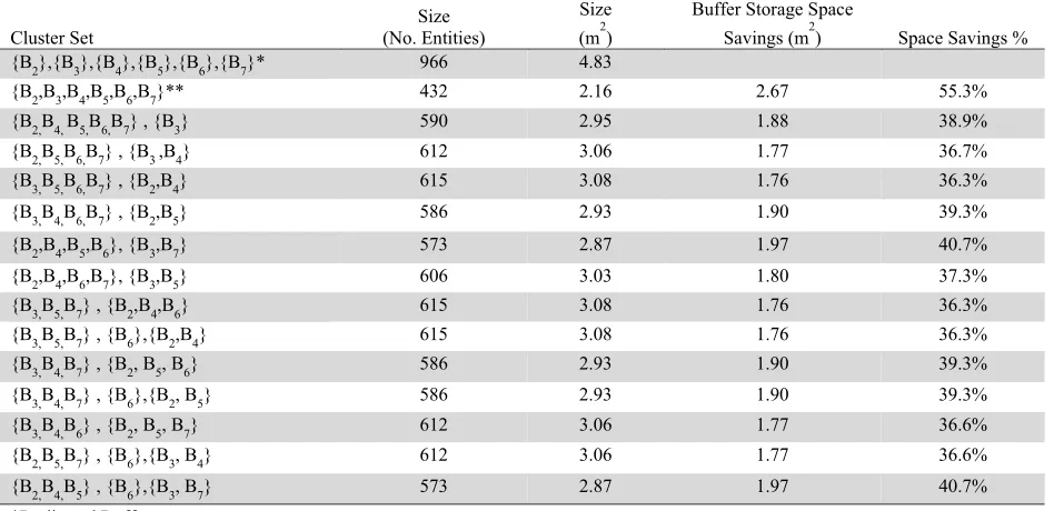
Fig. 8 (part a) is the original production line configuration. Batches of 80 come from inventory and enter the production line (B1). Batches of 80 are put on a pallet and shipped (B8). The top cluster configurations

considered by the facility based on buffer storage savings were then entered into a facility layout tool. The configuration shown in Fig. 8 (part b) was selected {B3, B4, B7}, {B2, B5, B6} resulting in a 39.3%

buffer storage savings (1.9 square meters).

Table 3

Buffer cluster sets and buffer storage savings

Cluster Set

Size (No. Entities)

Size (m2)

Buffer Storage Space

Savings (m2) Space Savings %

{B₂},{B₃},{B₄},{B₅},{B₆},{B₇}* 966 4.83

{B₂,B₃,B₄,B₅,B₆,B₇}** 432 2.16 2.67 55.3%

{B_2,B_4,B_5,B_6,B₇} , {B₃} 590 2.95 1.88 38.9%

{B_2,B_5,B_6,B₇} , {B₃,B₄} 612 3.06 1.77 36.7%

{B_3,B_5,B_6,B₇} , {B₂,B₄} 615 3.08 1.76 36.3%

{B_3,B_4,B_6,B₇} , {B₂,B₅} 586 2.93 1.90 39.3%

{B₂,B₄,B₅,B₆}, {B₃,B₇} 573 2.87 1.97 40.7%

{B₂,B₄,B₆,B₇}, {B₃,B₅} 606 3.03 1.80 37.3%

{B_3,B_5,B₇} , {B₂,B₄,B₆} 615 3.08 1.76 36.3%

{B_3,B_5,B₇} , {B₆},{B₂,B₄} 615 3.08 1.76 36.3%

{B_3,B_4,B₇} , {B₂, B₅, B₆} 586 2.93 1.90 39.3%

{B_3,B_4,B₇} , {B₆},{B₂, B₅} 586 2.93 1.90 39.3%

{B_3,B_4,B₆} , {B₂, B₅, B₇} 612 3.06 1.77 36.6%

{B_2,B_5,B₇} , {B₆},{B₃, B₄} 612 3.06 1.77 36.6%

{B_2,B_4,B₅} , {B₆},{B₃, B₇} 573 2.87 1.97 40.7%

*Dedicated Buffers

(13)

B2

(MB2 = 229)

S2 S3 S4

B3

(MB3 = 229)

B4

(MB4 = 92)

S5 S6

B5

(MB5 = 254)

S7

B6

(MB6 = 1

Transport Buffer)

B7

(MB7 = 121)

S1

B1

(Batches of 80)

B8

(Batches of 80

are put on a

pallet and

shipped)

Fig. 8(a). Serial production line

B1

(Batches of 80) S1

{B2,B5,B6} = 295

S2 S5 S6

S3 S7

{B3,B4,B7} = 291

B2 B5 B6

B3 B4

B7

S4

B8

Fig. 8(b). Production line with buffer clusters

As discussed in the introduction, Eq. (16) along with the objective function and constraints in Eqs. (18-20) can be used to conduct sensitivity analysis of the buffer cluster size by varying parameters such as server process time Ti and production demand K1.

Table 4

Wj buffer cluster sets and BBj values for each buffer cluster set (T2 = 3s)

W₁ = {B₂} W₂ ={B₃} W₃ = {B₄} W₄ = {B₅}

BB

1 = 305 BB2 = 115 BB3 = 92 BB4= 294

W

5 = {B6} W6 = {B7} W7 = {B2,B3} W8 = {B2,B4}

BB

5= 1 (Transport) BB6 =121 BB7 = 343 BB8 = 327

W

9 = {B2,B5} W10 = {B2,B6} W11= {B2, B7} W12={B3,B4}

BB

9 =363 BB10 = 306 BB11 = 313 BB12 = 183

W

13={B3,B5} W14 = {B3,B6} W15 = {B3,B7} W16 = {B4,B5}

BB

13 = 294 BB14 = 116 BB15 = 140 BB16 = 326

W

17={B4,B6} W18 = {B4,B7} W19={B5,B6} W20={B5,B7}

BB

17 = 93 BB18 = 126 BB19 =295 BB20=337

W

21={B6,B7} W22 = {B2,B3, B4} W23 = {B2,B3,B5} W24 = {B2,B3,B6}

BB

21=122 BB22 = 365 BB23 = 401 BB24 = 344

W

25 = {B2,B3,B7} W26 = {B2,B4,B5} W27 = {B2,B4,B6} W28 = {B2,B4,B7}

BB

25 = 351 BB26 = 385 BB27 = 328 BB28 = 335

W₂₉= {B_2,B_5,B₆} W₃₀= {B_2,B_5,B₇} W₃₁= {B_2,B_6,B₇} *W₃₂={B_3,B_4,B₅}

BB₂₉= 364 BB₃₀= 371 BB₃₁= 314 *BB₃₂= 358

W₃₃={B_3,B_4,B₆} W₃₄={B_3,B_4,B₇} W₃₅={B_3, B_5,B₆} W₃₆={B_3, B_5,B₇}

BB₃₃= 184 BB₃₄= 208 BB₃₅= 295 BB₃₆= 337

W

37={B3, B6,B7} W38={B4,B5,B6} W39={B4,B5,B7} W40={B4, B6,B7}

BB

37 = 141 BB38 = 327 BB39 = 360 BB40 = 127

W

41={B5, B6,B7} W42 = {B2,B3,B4,B5} W43 = {B2,B3,B4,B6} W44 = {B2,B3,B4,B7}

BB

41 = 338 BB42 = 423 BB43 = 366 BB44 = 373

W₄₅= {B_2,B_3,B_5,B₆} W₄₆= {B_2,B_3,B_5,B₇} W

47 = {B2,B3,B6,B7} W48 = {B2,B4,B5,B6}

BB₄₅= 402 BB₄₆= 409 BB

47 = 352 BB48 = 386

W

49 = {B2,B4,B5,B7} W50 = {B2,B4,B6,B7} W51 = {B2,B5,B6,B7} *W52 = {B3,B4,B5,B6}

BB

49 = 393 BB50 = 336 BB51 = 372 *BB52 = 359

W

53= {B3,B4,B5,B7} W54 = {B3,B4,B6,B7} W55 = {B3,B5,B6,B7} W56 = {B4,B5,B6,B7}

BB

53 = 384 BB54 = 209 BB55 = 338 BB56 = 361

W

57 = {B2,B3,B4,B5,B6} W58 = {B2,B3,B4,B5,B7} W59 = {B2,B3,B4,B6,B7} W60 = {B2,B3,B5,B6,B7}

BB₅₇= 424 BB₅₈= 431 BB₅₉= 374 BB₆₀= 410

W

61 = {B2,B4,B5,B6,B7} W62 = {B3,B4,B5,B6,B7} W63 = { B2,B3,B4,B5,B6,B7}

BB

(14)

Now the authors leverage the framework of the model and vary the process time of one server to demonstrate how the model can be used for sensitivity analysis. In this case, authors vary the process time of server S2 to three seconds, calculate the BBj values for each cluster set and show the buffer cluster

sets in Table 4. As before, the cells with bold text indicate that the cluster does not meet the space constraint and are the same cells that did not meet the space constraint in Table 2. If the cells are in italicized text, they used to meet the space constraint, but due to the change in the process times, no longer meet the constraint. The cells with a “*” indicate that the cluster exceeded space constraint in Table 2, but now meets the constraint in Table 4. The BBj values in red text indicate a change in the size

of the cluster from Table 2. Now the authors take the configurations from Table 3 and identify in Table 5 that there are configurations that now, with S2 equaling 3 seconds do not meet the space constraint (in

bold text). It is shown that the configuration selected with a process time S2 equaling 2 seconds,

{B3,B4,B7}, {B2, B5, B6}, with 586 entities, achieves a total buffer size of 572 entities when the process

time of S2 is 3 seconds. This scenario in italicized text in Table 5. So the initial buffer cluster set shown

in Fig. 8 can remain and still satisfy the space constraints when the process time of S2 varies from two to

three seconds.

Table 5

Buffer cluster sets and buffer storage savings with T2 at 2 and 3 seconds

Cluster Set

Size (No. Entities)

T2 =2s

Size (No. Entities)

T2 =3s

Size (m2) T2 =2s

Size (m2) T2 = 3s

Buffer Storage

Space Savings

(m2) T2= 2s

Buffer Storage

(m2) T2 = 3s

% T2 = 2 s

% T2 = 3 s

{B₂},{B₃},{B₄},{B₅},{B₆},{B₇}* 966 928 4.83 4.64

{B₂,B₃,B₄,B₅,B₆,B₇}** 432 432 2.16 2.16 2.67 2.48 55.3 53.5

{B2,B4, B5,B6,B7} , {B3} 590 509 2.95 2.55 1.88 2.10 38.9 45.2

{B2,B5,B6,B7} , {B3 ,B4} 612 555 3.06 2.78 1.77 1.87 36.7 40.2

{B_3,B_5,B_6,B₇} , {B₂,B₄} 615 665 3.08 3.33 1.76 1.32 36.3 28.3 {B_3,B_4,B_6,B₇} , {B₂,B₅} 586 572 2.93 2.86 1.90 1.78 39.3 38.4

{B2,B4,B5,B6}, {B3,B7} 573 526 2.87 2.63 1.97 2.01 40.7 43.3

{B₂,B₄,B₆,B₇}, {B₃,B₅} 606 630 3.03 3.15 1.80 1.49 37.3 32.1 {B_3,B_5,B₇} , {B₂,B₄,B₆} 615 665 3.08 3.33 1.76 1.32 36.3 28.3 {B_3,B_5,B₇} , {B₆},{B₂,B₄} 615 665 3.08 3.33 1.76 1.32 36.3 28.3

{B_3,B_4,B₇} , {B₂, B₅, B₆} 586 572 2.93 2.86 1.90 1.78 39.3 38.4

{B_3,B_4,B₇} , {B₆},{B₂, B₅} 586 572 2.93 2.86 1.90 1.78 39.3 38.4

{B_3,B_4,B₆} , {B₂, B₅, B₇} 612 555 3.06 2.78 1.77 1.87 36.6 40.2

{B_2,B_5,B₇} , {B₆},{B₃, B₄} 612 555 3.06 2.78 1.77 1.87 36.6 40.2

{B_2,B_4,B₅} , {B₆},{B₃, B₇} 573 526 2.87 2.63 1.97 2.01 40.7 43.3

*Dedicated Buffers

** Optimal Buffer Cluster without space constraints

5. Conclusion

(15)

Related studies are in progress that relax assumptions of the models in this paper and also expand configurations. In particular, studies in process consider unreliable machines. Another area of study is utilizing the model herein to consider when product size varies throughout the manufacturing process. The ability to extract state space models at any given time of interest is a rich area for Operations Research with several applications in industry.

References

Aghazadeh, S., Hafeznezami, S., Najjar L., and Huq, Z. (2011). The influence of work-cells and facility layout on the manufacturing efficiency. Journal of Facilities Management, 9(3), 213-224. Becker, C., & Scholl, A. (2006). A survey on problems and methods in generalized assembly line

balancing. European journal of operational research, 168(3), 694-715.

Chan, F. T. S., & Ng, E. Y. H. (2002). Comparative evaluations of buffer allocation strategies in a serial production line. The International Journal of Advanced Manufacturing Technology, 19(11), 789-800. Charharsooghi, S.K. and Nahavandi, N. (2003). Buffer allocation problem, a heuristic approach. Scientia

Iranica, 10(4), 401-409.

Chow, W. M. (1987). Buffer capacity analysis for sequential production lines with variable process times. International Journal of Production Research,25(8), 1183-1196.

Enginarlar, E., Li, J., & Meerkov, S. M. (2005). How lean can lean buffers be?. IIE Transactions, 37(4), 333-342.

Enginarlar, E., Li, J., Meerkov, S. M., & Zhang, R. Q. (2002). Buffer capacity for accommodating machine downtime in serial production lines. International Journal of Production Research, 40(3), 601-624.

Gershwin, S. B. (1987). An efficient decomposition method for the approximate evaluation of tandem queues with finite storage space and blocking. Operations research, 35(2), 291-305.

Gershwin, S. B., & Schor, J. E. (2000). Efficient algorithms for buffer space allocation. Annals of

Operations Research, 93(1-4), 117-144.

Govil, M. K., & Fu, M. C. (1999). Queueing theory in manufacturing: A survey. Journal of

manufacturing systems, 18(3), 214.

Ichikawa, H. (2009, December). Simulating an applied model to optimize cell production and parts supply (Mizusumashi) for laptop assembly. In Winter Simulation Conference (pp. 2272-2280). Winter Simulation Conference.

Kouikoglou, V. S., & Phillis, Y. A. (1991). An exact discrete-event model and control policies for production lines with buffers. Automatic Control, IEEE Transactions on, 36(5), 515-527.

Kouikoglou, V. S., & Phillis, Y. A. (1994). Discrete event modeling and optimization of unreliable production lines with random rates. Robotics and Automation, IEEE Transactions on, 10(2), 153-159. Kouikoglou, V. S., & Phillis, Y. A. (1995). An efficient discrete-event model for production networks of

general geometry. IIE transactions, 27(1), 32-42.

Li, J., E. Blumenfeld, D., Huang, N., & M. Alden, J. (2009). Throughput analysis of production systems: recent advances and future topics.International Journal of Production Research, 47(14), 3823-3851. Lim, J. T., Meerkov, S. M., & Top, F. (1990). Homogeneous, asymptotically reliable serial production

lines: theory and a case study. Automatic Control, IEEE Transactions on, 35(5), 524-534..

Liu, C. M. and Lin, C. L. (1994). Performance evaluation of unbalanced serial production lines.

International Journal of Production Research, 32(12),2897–2914.

Logendran, R., & Karim, Y. (2003). Design of manufacturing cells in the presence of alternative cell locations and material transporters. Journal of the Operational Research Society, 54, 1059-1075. Matta, A., Runchina, M., & Tolio, T. (2006). Automated flow lines with shared buffer. In Stochastic

Modeling of Manufacturing Systems (pp. 99-120). Springer Berlin Heidelberg.

Morrison, J. R. (2010). Deterministic flow lines with applications. Automation Science and Engineering,

(16)

Ramirez-Serrano, A., & Benhabib, B. (2000). Supervisory control of multiworkcell manufacturing systems with shared resources. Systems, Man, and Cybernetics, Part B: Cybernetics, IEEE

Transactions on, 30(5), 668-683.

Senanayake, C. D., & Subramaniam, V. (2013). Analysis of a two-stage, flexible production system with unreliable machines, finite buffers and non-negligible setups. Flexible Services and Manufacturing Journal, 25(3), 414-442.

So, K. C. (1989). Allocating buffer storages in a flexible manufacturing system. International journal of

flexible manufacturing systems, 1(3), 223-237.

Wei, K. C., Tsao, Q. Q., & Otto, N. C. (1989, December). Estimation of buffer size using stochastic approximation methods. In Decision and Control, 1989., Proceedings of the 28th IEEE Conference on (pp. 1066-1068). IEEE.

Yamashita, H., & Altiok, T. (1998). Buffer capacity allocation for a desired throughput in production lines. IIE transactions, 30(10), 883-892.

Youssef, A. M., & ElMaraghy, H. A. (2007). Optimal configuration selection for reconfigurable manufacturing systems. International Journal of Flexible Manufacturing Systems, 19(2), 67-106.

Appendix A. Proof for minimum cluster size

Lemma 1: Minimum size for cluster Wjsuch that no overflows occur takes place when at least one of

the buffers Biin cluster Wj has reached the maximum number of entities, MBi.

Take buffers Bk and Bp that are in cluster Wj and output to servers Skand Sprespectively where k < p, and

the constraints MTk-1 < MTk and MTp-1 < MTp hold. Recall from Corollary 2 that when MTk-1 = MTk or

MTp-1 = MTp, the buffer size is 1. For the proof, the authors observe the buffer inventory profiles of Bk

and Bp at three specific time intervals of the buffer inventory covering the time from the first arrival to

buffer Bk to the last departure from buffer Bp as shown in Fig. 9. In addition, authors also observe when

buffers Bk and Bp are sequential (p = k+1) and when they are not (p > k +1). Fig. 9 shows the case when

p = k+1. As p > k+1, the buffer profiles drift apart and the overlap in Time Interval 3 decreases until no overlap exists.

Fig. 9. Buffer profiles of Bk and Bp and time Intervals 1 through 3 for p = k + 1

Time Interval 1: τk-1 < t < t2 Bk̅ (Bk and Bp are increasing; Bk has reached a maximum)

Buffer Bk has its first arrival at τ_k-1 and increases until it reaches MBk. Buffer Bp has its first arrival at

τp-1 and increases until it reaches its maximum, MBp. For Buffers Bk and Bpwhere p = k+1, τ_p-1-τ_k-1 =

Tk. Thus, buffer Bp starts increasing Tk seconds after the first arrival to buffer Bk. When p > k+1, τ_p-1

τk-1is greater than Tk meaning that time of the first arrival of Bp approaches and can exceed time interval

[ ̅ , ̅ when Bk is maximum. When buffer Bkis at its maximum (MBk), buffer Bp is increasing in

size, while after reaching MBk, buffer Bkbegins to decline. Therefore, a possible buffer cluster maximum

(17)

Time Interval 2: t̅1 Bp < t < τp-1+ K1-1 *MTp (Bk is decreasing and reaches zero; Bp has reached its

maximum and begins to decline including its last departure)

The last arrival to buffer Bp at time τ K1 1 ∗ MT

The last departure of buffer Bk occurs at time τ K1 1 ∗ MT

Subtract these times to get:

τ K1 1 ∗ MT τ K1 1 ∗ MT =

τ τ K1 1 ∗ MT K1 1 ∗ MT =

τ τ 1 1 ∗ MT MT

(A.1)

For Buffers Bk and Bp where p = k+1 then MT MT = 0 and τ τ = Tk then (A.1) equals

Tk. Therefore, the last departure of Bk occurs Tk seconds prior to the last arrival to buffer Bp. Thus Bk is

reaches zero while Bp is at a maximum. When p > k+1, then τ τ is greater than Tk and MTk <

MTp-1, therefore (K1-1)* MT MT > 0, resulting in (A.1) being greater than Tk. Therefore, a

possible buffer cluster maximum between buffers Bk and Bp occurs at MBp.

Time Interval 3: ̅ < t < ̅ (Bk is decreasing; Bp is increasing but has not reached a maximum)

At time ̅ , Bk has experienced its last arrival (K1) and it has reached a maximum MBk. Therefore,

after this time, only departures occur. Thus in essence, MBk indicates the number of departures that are

left for buffer Bk until it reaches zero. During this time interval, buffer Bp is increasing (it hasn’t reached

a maximum yet), meaning it has both arrivals and departures. When p = k+1, MTk = MTp-1 indicating

that the number of departures remaining at buffer Bk , MBk , is also the number of entities still to arrive at

buffer Bp and they occur at the same time. However, given that Bp is increasing and hasn’t reached a

maximum, it is also experiencing departures at a rate of MTp. During this time interval, the quantity of

inventory of buffer Bk declines from MBk to zero. Although Buffer Bp entities arrive at the same rate as

buffer Bk departures, its inventory increases more slowly than the decline of departures from buffer Bk

given buffer Bpalso has entities departing at a rate of MTp during this time interval. Therefore the sum

of the inventory profiles of buffer Bk and Bp during this time interval will not exceed the maximum

inventory observed in time interval (1) or (2) described above. When p > k + 1, buffer Bp has its first

entity arriving even later than in the p = k+1 case. Although the decline of buffer Bk remains the same,

buffer Bp starting arrival approaches the time when buffer BkapproachesMBk and the summation of the

two inventory profiles will not exceed the maximum inventory observed in time interval (1) or (2) described above. Based on results of the analysis for each of the time intervals, the union of time intervals in (A.2) for each buffer must be searched to find the maximum buffer cluster size BBj.

t ϵ t1 B1, ̅ t2 B1̅ ∪t1B2, ̅ t̅2 B2 ∪… t1Bi, ̅ t2 Bi̅ ∪… t1B̅ N, t̅2 BN (A.2)

Appendix B. Computational and solution time savings

Table 6 shows that for this case study, 26 critical time steps were identified to measure the buffer size, resulting in 26 calculations. For Buffer B6, because MTi-1 > MTi , no time interval to detect the maximum

buffer size is required because buffer size required is always 1 (as discussed in Corollary 2, this is a transport buffer).

(18)

K1 or production demand is also varied (from 100 to 300) such that it would cover a production shift interval spread of 8 to 12 hours.

Table 6

Number of time steps for required buffer size computations

Element B_i B₂ B₃ B₄ B₅ B₆ B₇

t1Bi̅ 458 917 1831 2292 0 6434

t2Bi ̅ 459 918 1836 2307 0 6438

t2Bi̅ t1Bi̅

Total: B2 – B7 = 26 1 1 5 15 0 4

Table 7

Calculation and computation time savings varying K1