Misclassiﬁcation in Binary Choice Models with Sample Selection

(1)

Article

Misclassification in Binary Choice Models with

Sample Selection

Maria Felice Arezzo *,† and Giuseppina Guagnano†

Department of Methods and Models for Economics, Territory and Finance - Sapienza University of Rome Via del Castro Laurenziano 9, 00161 Rome, Italy

* Correspondence: [email protected]; Tel.: +39-06-49766424 † These authors contributed equally to this work.

Received: 7 January 2019; Accepted: 17 July 2019; Published: 24 July 2019

Abstract: Most empirical work in the social sciences is based on observational data that are often both incomplete, and therefore unrepresentative of the population of interest, and affected by measurement errors. These problems are very well known in the literature and ad hoc procedures for parametric modeling have been proposed and developed for some time, in order to correct estimate’s bias and obtain consistent estimators. However, to our best knowledge, the aforementioned problems have not yet been jointly considered. We try to overcome this by proposing a parametric approach for the estimation of the probabilities of misclassification of a binary response variable by incorporating them in the likelihood of a binary choice model with sample selection.

Keywords:misclassified dependent variable; sample selection bias; undeclared work

1. Introduction

Most empirical work in the social sciences is based on observational data that are often incomplete, and therefore unrepresentative of the population of interest, and/or affected by measurement errors. There are many types of selection mechanisms that result in a non-random sample. Some of them are due to sample design, while others depend on the behavior of the units being sampled, other than non-response or attrition. In the first case, data are usually missing on all the variables of interest; for example, in estimating a saving function for all the families of a given country, a bias would arise if only families whose household head shows certain characteristics were sampled. However, when causes of missingness are appropriately exogenous, using a sub-sample has no serious consequences.

In the second case, instead, there is a self-selection of the sample units and data availability on a key variable depends on the behavior of the units about another variable. The classical example is that of the linear wage equation where we want to estimate the expected wage of an individual using a set of exogenous characteristics (gender, age, education, etc.). The key problem is that, in regressing wages on the characteristics ofemployedindividuals, we are not making inferences for the population as a whole. In fact, those in employment are a selected sample of the population and their wages are higher than those not in the labor force would have. Hence, the results will tend to be biased and inconsistent (sample selection bias). To avoid this problem, we need to take into account the selection mechanism by which an individual decides to take a job and then receives a wage.

As is well known,Heckman(1979) proposed a useful framework for handling estimation when the sample is subject to a selection mechanism, trying to correct for non-randomly selected data in a two-model hierarchy where, on the first level, a binary selection equation determines whether a particular observation will be available for the second level (outcome equation). In the original framework, the dependent variable in the outcome equation (the wage equation in the above example)

(2)

is continuous and can be explained by a linear regression model with a normal random component. In addition to the output equation, a selection equation describes the selection rule by means of a binary choice model (probit).

The original Heckman’s model was extended in many directions and a survey would be beyond the scope of this paper, but the interested reader can refer to the works ofVella(1998) andLee(2007). To our purposes, the relevant framework is the one where both the output and the selection equations are defined as a binary choice model (Dubin and Rivers 1989). The likelihood function takes into account the selection mechanism and allows for consistent estimates of the parameters of interest (i.e., the coefficients of the selection and the outcome equations and the correlation coefficient of the two processes).

In many disciplines, however, binary data are frequently misclassified. Misclassification of a binary variable means that an observation with a true value of 0 is observed as 1 or an observation that is truly a 1 is observed as a 0. This mistake could easily happen, for example, during an interview if the respondent misunderstands the question or the interviewer simply checks the wrong box. In employment analysis, tenure responses can be measured with errors because respondents have poor recall or confuse a change in position with an actual job change (Hausman et al. 1998); in this framework, evidence from validation studies (e.g., (Mellow and Sider 1983)) suggests that 20 percent of one-digit occupational choices are misclassified. Finally, as underlined by the social psychology literature, respondents tend to over-report socially desirable behaviors and under-report socially undesirable ones (Loftus 1975). For example, in surveys on voting behavior, some respondents state that they have voted, while they did not. Empirical evidence of this behavior was provided byKatz and Katz(2010): using auxiliary information from the American National Elections, they discovered that, depending on the election year, between 13.6% and 24.6% of the respondents claiming to have voted did in fact not vote according to the public records.

This kind of misreporting might become even more frequent when the response variable refers to characteristics subjected to a moral judgment; it is the case, for example, of the dependent variable considered in the application discussed in Section4(having, or not, carried out some undeclared activities), but also when the dependent variable refers to one’s attitude to tax evasion, racism, drug or games addiction, and religious belief.

Ignoring the presence of misclassification is not trivial; in fact, when traditional estimation methods (e.g., logit or probit) are used in binary choice contexts with a misclassified dependent variable, the resulting estimates are inconsistent.

Previous work on misclassified dependent variables in discrete choice models follows two approaches. In the first, supplemental data are used to verify the accuracy of responses. In the work of Chua and Fuller(1987), a parametric model that incorporates all possible J(J−1)misclassification of aJ-level outcome variable is developed. This approach has been seldom used because it is very data demanding, as a minimum of three independent sets of survey responses obtained by re-interviewing the original respondents are required. A similar approach, based on a conditional logit procedure, was proposed byPoterba and Summers(1995). It also incorporates all possible misclassification and the estimation of the misclassification probabilities is done by analyzing the divergences between interview and re-interview outcomes.

(3)

occupational choice, and the other the extent of misclassification in occupational data. However, this proposal is specific for the study of the determinants of occupational choices and for estimating the effects of occupation-specific human capital on wages. On the contrary, Hausman et al.’s proposal is quite general and applicable in several contexts. Therefore, we start from their work, incorporating the other source of inconsistency coming from sample selection. We use a parametric approach to simultaneously estimate the parameters of the selection and of the outcome equations, the correlation between them and the probabilities of misclassification.

2. The Model

Let us first introduce some notations and briefly illustrate the sample selection framework with a binary choice model for both the selection and the output equations (Dubin and Rivers 1989).

We start with two observable binary variables: the dependent variable of the outcome equation Yand the one of the selection equationS. They can be seen as the observable proxies of two latent (unobservable) variables,Y∗andS∗, characterizing the output and the selection equations respectively. The model, in its general form, is:

Y_i∗=X1iβ+e1i (1a)

S∗_i =X2iθ+e2i (1b)

whereXi= (X1i,X2i)is a vector of exogenous variables (namely,X1iforY_i∗andX2iforS∗_i), containing all the relevant covariates,βandθare the vectors of regression coefficients, ande1i ande2iare the disturbances, assumed in general related withcorr(e1,e2) =ρ. Note that for the model in Equations (1a) and (1b) to be identified, we can rely either on nonlinearity (typically assuming a joint normality of

(e1,e2)) or on an exclusion restriction that translate in a non-full overlapping ofX1iandX2i; that is, the covariates of the selection and outcome equations must differ for at least one variable. The latter condition is necessary only when there are reasons to doubt that the nonlinearity holds.

We can now define the observable binary variablesYiandSias:

Yi= (

1 ifY_i∗>0

0 otherwise (2)

Si= (

1 ifS∗_i >0

0 otherwise (3)

The p.d.f. ofYiandSiare Bernoulli, with probability of success depending on the parametersβ andθ, respectively.

The model in Equation (3) defines the mechanism which governs the censoring process: we can observeYiif and only ifSi=1. On the contrary, ifSi=0,Yiwill be missing. Note that the selection mechanism affects the estimates only whenρis nonzero.

In the general case with nonzeroρ, if we were to estimate the parameters of Equation (1a) without considering the selection process (Equation (1b)), that is omitting information aboutS∗_i, a problem of inconsistency would arise (see, for example, (Cameron and Trivedi 2005), for further details).

The appropriate likelihood function for the model in Equations (1a) and (1b) is:

L(η) = n

∏

i=1

h

Pr(S∗_i <0)i1−Si·hPr(Yi=yi|S∗i >0)·Pr(Si∗>0) iSi

=

n

∏

i=1

h

1−_Sπ(Xi) i1−Si

·hPr(Yi =yi|Si =1)·Sπ(Xi) iSi

(4)

whereη= (β,θ,ρ)is the vector of parameters to be estimated,yi=0, 1 and the functionSπ(·)gives the probability that an observation is uncensored.

Now, if we assume that:

e1i e2i

!

∼ N ID "

0 0

!

, 1 ρ

ρ 1

!#

(5)

and putP(Yi =1|Si=1) =Yπ(Xi), we can compute the probabilitiesP(Si=0) =1−Sπ(X2i)and the joint probabilitiesP(Yi=yi,Si=1)in Equation (4) as follows:

Pr(Si=0) =1−Sπ(X2i) =Φ −θ0X2i (6)

Pr(Yi =1,Si=1) =Pr(Yi =1|Si =1)·Pr(Si =1) =Yπ(Xi)·Sπ(X2i)

=Φ2(X1iβ,X2iθ,ρ) (7)

Pr(Yi =0,Si=1) =Pr(Yi =0|Si =1)·Pr(Si =1) = (1−Yπ(Xi))·Sπ(X2i)

=Φ2(−X1iβ,X2iθ,ρ) (8)

whereΦandΦ2are c.d.f. of the univariate and the bivariate normal, respectively.

Now, let us suppose thatYican be misclassified, that is some true ones are observed as zeros, and some true zeros are observed as ones. It follows that what we observe can differ from the true proxy of the response variable of the outcome equation. Let us denoteobsYi as the observed binary variable affected by error, andTYias the true response variable of Equation (2). Following Hausman et al.(1998), we assume that the probability of misclassification depends on the value ofTYi, but is otherwise independent of the covariatesX1if conditioned onTYi. To be more specific, we set the following misclassification probabilities:

α0=Pr(obsYi =1|TYi =0) (9)

α1=Pr(obsYi =0|TYi =1) (10)

withα0+α1<1.

The probability that a true zero is misclassified as a one is given byα0; the probability that a true one is misclassified as a zero is given byα1. The stochastic mechanism that determines the values of the observed dependent variableobsYbecomes:

Pr(obsYi=1|Si =1,Xi) =

Pr(obsYi=1|Si =1,Xi,TYi=1)Pr(TYi=1|Si=1,Xi) +

+Pr(_obsYi =1|Si=1,Xi,TYi =0)Pr(TYi=0|Si =1,Xi)

= (1−α0−α1)Pr(TYi=1|Si =1,Xi) +α0 (11)

where Pr(TYi=1|Si=1,Xi) =TYπ(Xi)is the homologous ofYπ(Xi)in Equations (7) and (8). Obviously, we can put:

Pr(obsYi =0|Si=1,Xi) =1−Pr(obsYi=1|Si=1,Xi)

=1−α0−(1−α0−α1)Pr(TYi=1|Si=1,Xi) (12)

(5)

logL(γ) = n

∑

i=1

(1−Si)·logΦ(−X2iθ) +

Si·log "

α0Φ(X2iθ) + (1−α0−α1)Φ2(X1iβ,X2iθ,ρ)

#obsYi +

Si·log "

(1−α0)Φ(X2iθ)−(1−α0−α1)Φ2(X1iβ,X2iθ,ρ)

#1−obsYi

3. Simulation Results

In this section, we present Monte Carlo simulations done to evaluate finite sample performances of the proposed model. We consider the following generating model:

Y_i∗=−1+0.2X11i+1.5X12i−0.6X13i+e1i S∗_i =θ0+0.8X21i−0.5X22i+e2i

For the outcome equation, we mimicHausman et al.(1998); in particular,X11 is drawn from a lognormal,X12is a dummy variable equal to one with probability 1/3 andX13is a uniform(0, 1). In addition, the vector of parametersβis identical to theirs. For the selection equation, we have drawn bothX21andX22from a standard normal distribution. The choice ofθ0in{0.5; 2.18}is to ensure a medium and low amount of censored data (approximately 30% and 5%, respectively).

We performed 200 replications with samples of sizen=5000. We choseρ∈ {−0.8;−0.2; 0.2; 0.8} and the following pairs of misclassification probabilities:(α0=0.02,α1=0.02)and(α0=0.05,α1=0.2).

We compared four models: the simple probit, a model that corrects for sample selection only (named SS in the following), a model that corrects for misclassification only (MIS) and a model that corrects for both sample selectionandmisclassification (MIS-SS).

The results, reported in Tables1–4, allow evaluating the models’ performances by comparing the average estimates and mean squared error (MSE) as well as the coverages of the confidence intervals. MIS-SS has very good values for all indicators, along all simulation settings. In the following, we focus on the parameters of the outcome equation, being those of main interest.

With regards to probit estimates, in accordance withHausman et al. (1998), we find biased estimates. In particular, the average relative bias1, spans from 0.1% to 42% of the parameter true value, depending on the coefficient and on data generating schemes. As expected, the probit model performance improves with low levels of misclassification and censoring.

Correcting for sample selection (SS) induces the relative bias under 13%, no matter the value ofρ, if the misclassification probabilities are low; in the other cases, the bias spans from 6% to 44%.

When correcting for misclassification (MIS), the relative bias considerably reduces (around 5%) only ifρ is moderate. However, as expected, when the correlation between the outcome and the selection equation errors is higher, the bias reaches 15–20% with a peak of over 50% for the intercept. Correcting for both types of error leads to an improvement in estimation: the MIS-SS model bias spans from 0.04% to 12% of the parameter true value, outperforming all others.

Looking at the coverages, MIS-SS is almost always the best model when the misclassification probabilities are both at 2%. When the misclassification probabilities raise (α0=0.05 andα1=0.2), MIS dominates all models, but MIS-SS is the second best; furthermore, the performance of MIS-SS improves as the censoring percentage increases.

Similar considerations partially apply to the MSEs, although the evaluations are more difficult as the results are more diversified across the parameters space.

1 _{For each replication}_k_{, we compute the following relative difference between the estimate and the parameter value}

(6)

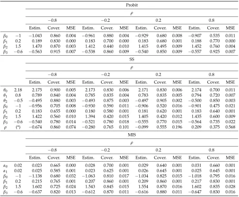
Table 1.Monte Carlo simulation results: average values of estimates, coverage of confidence intervals and MSEs. Data generating scheme:n=5000,α0=α1=0.02,

ρ∈ {±0.2;±0.8}; censored observations approximately 5%.

Probit

ρ

−0.8 −0.2 0.2 0.8

Estim. Cover. MSE Estim. Cover. MSE Estim. Cover. MSE Estim. Cover. MSE

β0 −1 −1.043 0.860 0.004 −0.961 0.880 0.004 −0.929 0.680 0.008 −0.907 0.535 0.011

β1 0.2 0.189 0.830 0.000 0.183 0.700 0.000 0.183 0.680 0.001 0.188 0.770 0.000

β2 1.5 1.470 0.870 0.003 1.412 0.440 0.010 1.415 0.495 0.009 1.452 0.760 0.004

β3 −0.6 −0.563 0.915 0.007 −0.538 0.860 0.009 −0.540 0.850 0.009 −0.557 0.925 0.007

SS

ρ

−0.8 −0.2 0.2 0.8

θ0 2.18 2.175 0.900 0.005 2.173 0.830 0.006 2.171 0.830 0.006 2.174 0.700 0.011

θ1 0.8 0.789 0.840 0.004 0.785 0.835 0.004 0.783 0.835 0.005 0.794 0.720 0.007

θ2 −0.5 −0.495 0.880 0.003 −0.493 0.875 0.003 −0.497 0.905 0.002 −0.500 0.850 0.003

β0 −1 −0.956 0.705 0.008 −0.930 0.590 0.011 −0.906 0.520 0.016 −0.901 0.475 0.021

β1 0.2 0.183 0.655 0.000 0.180 0.580 0.001 0.181 0.620 0.001 0.183 0.640 0.001

β2 1.5 1.422 0.560 0.010 1.394 0.420 0.015 1.405 0.420 0.012 1.435 0.600 0.009

β3 −0.6 −0.540 0.780 0.014 −0.521 0.780 0.018 −0.555 0.770 0.015 −0.564 0.735 0.022

ρ (*) −0.674 0.860 0.074 −0.280 0.765 0.101 −0.099 0.555 0.196 0.209 0.375 0.568

MIS

ρ

−0.8 −0.2 0.2 0.8

α0 0.02 0.023 0.665 0.000 0.028 0.700 0.001 0.029 0.640 0.001 0.031 0.660 0.001

α1 0.02 0.025 0.585 0.001 0.023 0.625 0.001 0.026 0.645 0.001 0.025 0.645 0.001

β0 −1 −1.138 0.680 0.032 −1.063 0.810 0.017 −1.034 0.825 0.015 −1.018 0.795 0.016

β1 0.2 0.215 0.765 0.001 0.207 0.860 0.001 0.209 0.860 0.001 0.217 0.830 0.001

β2 1.5 1.602 0.725 0.024 1.543 0.845 0.015 1.554 0.870 0.016 1.602 0.835 0.028

(7)

Table 1.Cont.

MIS-SS

ρ

−0.8 −0.2 0.2 0.8

α0 0.02 0.021 0.640 0.143 0.022 0.635 0.143 0.018 0.565 0.143 0.014 0.465 0.144

α1 0.02 0.014 0.445 0.143 0.010 0.355 0.144 0.007 0.225 0.144 0.009 0.225 0.144

θ0 2.18 2.190 0.910 0.004 2.184 0.905 0.004 2.186 0.960 0.004 2.190 0.940 0.003

θ1 0.8 0.804 0.915 0.002 0.799 0.925 0.002 0.802 0.955 0.002 0.806 0.935 0.002

θ2 −0.5 −0.504 0.900 0.002 −0.503 0.960 0.002 −0.502 0.970 0.002 −0.508 0.940 0.001

β0 −1 −1.028 0.885 0.010 −1.022 0.885 0.013 −1.004 0.910 0.009 −0.989 0.835 0.009

β1 0.2 0.200 0.865 0.001 0.197 0.880 0.001 0.194 0.875 0.000 0.193 0.820 0.000

β2 1.5 1.513 0.875 0.010 1.494 0.810 0.013 1.475 0.830 0.010 1.472 0.735 0.011

β3 −0.6 −0.594 0.905 0.015 −0.587 0.890 0.011 −0.579 0.905 0.010 −0.578 0.895 0.010

ρ (*) −0.758 0.965 0.016 −0.199 0.975 0.030 0.190 0.940 0.035 0.741 0.935 0.024

(*): see the reference values at the top of the columns.

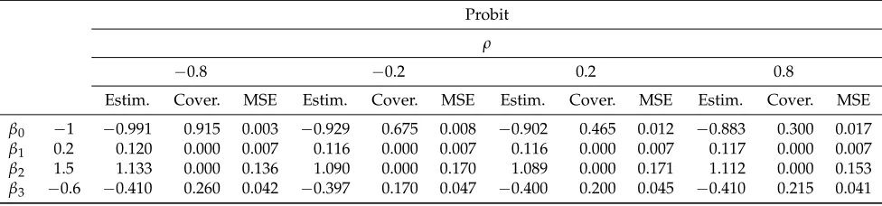
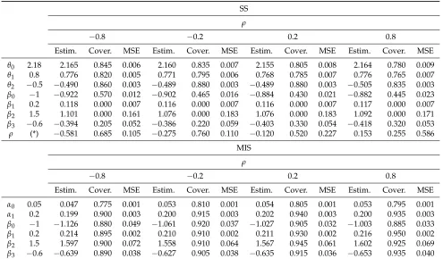
Table 2. Monte Carlo simulation results: average values of estimates, coverage of confidence intervals and MSEs. Data generating scheme:n=5000,α0 =0.05;

α1=0.2,ρ∈ {±0.2;±0.8}; censored observations approximately 5%.

Probit

ρ

−0.8 −0.2 0.2 0.8

β0 −1 −0.991 0.915 0.003 −0.929 0.675 0.008 −0.902 0.465 0.012 −0.883 0.300 0.017

β1 0.2 0.120 0.000 0.007 0.116 0.000 0.007 0.116 0.000 0.007 0.117 0.000 0.007

β2 1.5 1.133 0.000 0.136 1.090 0.000 0.170 1.089 0.000 0.171 1.112 0.000 0.153

(8)

Table 2.Cont.

SS

ρ

−0.8 −0.2 0.2 0.8

θ0 2.18 2.165 0.845 0.006 2.160 0.835 0.007 2.155 0.805 0.008 2.164 0.780 0.009

θ1 0.8 0.776 0.820 0.005 0.771 0.795 0.006 0.768 0.785 0.007 0.776 0.765 0.007

θ2 −0.5 −0.490 0.860 0.003 −0.489 0.880 0.003 −0.489 0.880 0.003 −0.505 0.835 0.003

β0 −1 −0.922 0.570 0.012 −0.902 0.465 0.016 −0.884 0.430 0.021 −0.882 0.445 0.023

β1 0.2 0.118 0.000 0.007 0.116 0.000 0.007 0.116 0.000 0.007 0.117 0.000 0.007

β2 1.5 1.101 0.000 0.161 1.076 0.000 0.183 1.076 0.000 0.183 1.092 0.000 0.171

β3 −0.6 −0.394 0.205 0.052 −0.386 0.220 0.059 −0.403 0.330 0.054 −0.418 0.320 0.053

ρ (*) −0.581 0.685 0.105 −0.275 0.760 0.110 −0.120 0.520 0.227 0.153 0.255 0.586

MIS

ρ

−0.8 −0.2 0.2 0.8

α0 0.05 0.047 0.775 0.001 0.053 0.810 0.001 0.054 0.805 0.001 0.053 0.795 0.001

α1 0.2 0.199 0.900 0.003 0.200 0.915 0.003 0.202 0.940 0.003 0.200 0.935 0.003

β0 −1 −1.126 0.880 0.049 −1.061 0.920 0.037 −1.027 0.905 0.032 −1.003 0.885 0.033

β1 0.2 0.214 0.895 0.002 0.210 0.910 0.002 0.211 0.930 0.002 0.216 0.950 0.002

β2 1.5 1.597 0.900 0.072 1.558 0.910 0.064 1.567 0.945 0.061 1.602 0.925 0.069

(9)

Table 2.Cont.

MIS-SS

ρ

−0.8 −0.2 0.2 0.8

α0 0.05 0.028 0.425 0.122 0.040 0.355 0.121 0.037 0.350 0.121 0.026 0.245 0.121

α1 0.2 0.149 0.660 0.037 0.140 0.520 0.037 0.130 0.465 0.037 0.119 0.400 0.038

θ0 2.18 2.180 0.945 0.004 2.179 0.935 0.004 2.181 0.925 0.005 2.186 0.960 0.003

θ1 0.8 0.795 0.940 0.002 0.792 0.920 0.002 0.795 0.920 0.003 0.801 0.900 0.002

θ2 −0.5 −0.501 0.915 0.002 −0.500 0.935 0.002 −0.500 0.915 0.002 −0.507 0.925 0.002

β0 −1 −0.963 0.730 0.028 −1.003 0.765 0.047 −1.016 0.615 0.175 −0.982 0.600 0.189

β1 0.2 0.180 0.600 0.003 0.185 0.485 0.005 0.174 0.420 0.012 0.178 0.375 0.010

β2 1.5 1.402 0.560 0.111 1.435 0.370 0.142 1.434 0.395 0.289 1.398 0.305 0.281

β3 −0.6 −0.549 0.705 0.091 −0.579 0.660 0.077 −0.522 0.620 0.304 −0.527 0.540 0.055

ρ (*) −0.666 0.835 0.067 −0.301 0.785 0.121 −0.028 0.750 0.215 0.389 0.605 0.375

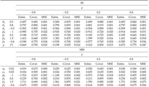
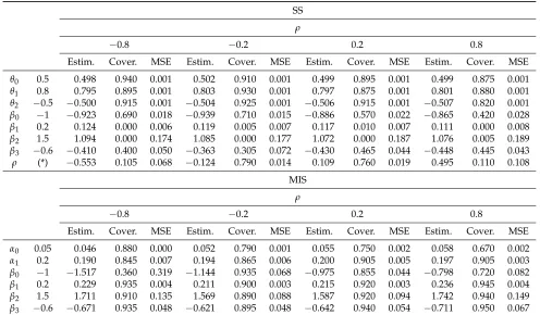
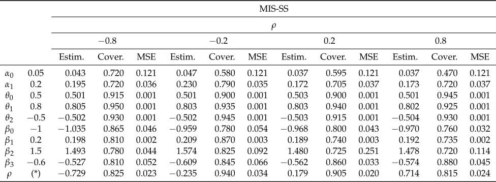
Table 3.Monte Carlo simulation results: average values of estimates, coverage of confidence intervals and MSEs. Data generating scheme:n=5000,α0=α1=0.02,

ρ∈ {±0.2;±0.8}; censored observations approximately 30%.

Probit

ρ

−0.8 −0.2 0.2 0.8

β0 −1 −1.376 0.000 0.146 −1.029 0.915 0.005 −0.872 0.360 0.020 −0.702 0.000 0.092

β1 0.2 0.200 0.920 0.000 0.183 0.765 0.001 0.184 0.775 0.001 0.202 0.915 0.000

β2 1.5 1.547 0.870 0.006 1.412 0.575 0.011 1.420 0.635 0.010 1.564 0.810 0.007

(10)

Table 3.Cont.

SS

ρ

−0.8 −0.2 0.2 0.8

θ0 0.5 0.497 0.885 0.001 0.500 0.870 0.001 0.499 0.880 0.001 0.495 0.840 0.001

θ1 0.8 0.797 0.890 0.001 0.799 0.870 0.001 0.801 0.915 0.001 0.797 0.860 0.002

θ2 −0.5 −0.503 0.905 0.001 −0.506 0.890 0.001 −0.504 0.890 0.001 −0.509 0.830 0.001

β0 −1 −0.985 0.755 0.022 −0.925 0.760 0.020 −0.912 0.720 0.020 −0.914 0.665 0.031

β1 0.2 0.188 0.715 0.001 0.181 0.720 0.001 0.183 0.735 0.001 0.185 0.665 0.001

β2 1.5 1.413 0.640 0.015 1.383 0.435 0.021 1.399 0.520 0.016 1.431 0.645 0.018

β3 −0.6 −0.549 0.770 0.034 −0.538 0.700 0.030 −0.577 0.765 0.024 −0.585 0.730 0.036

ρ (*) −0.669 0.750 0.032 −0.198 0.835 0.014 0.163 0.850 0.013 0.673 0.775 0.047

MIS

ρ

−0.8 −0.2 0.2 0.8

α0 0.02 0.019 0.675 0.000 0.029 0.625 0.001 0.030 0.645 0.001 0.038 0.540 0.001

α1 0.02 0.024 0.505 0.001 0.024 0.550 0.001 0.025 0.635 0.001 0.022 0.500 0.000

β0 −1 −1.514 0.015 0.281 −1.149 0.810 0.042 −0.973 0.760 0.018 −0.813 0.495 0.052

β1 0.2 0.229 0.760 0.002 0.210 0.870 0.001 0.211 0.895 0.001 0.236 0.625 0.002

β2 1.5 1.711 0.690 0.062 1.561 0.870 0.021 1.559 0.885 0.020 1.731 0.590 0.075

(11)

Table 3.Cont.

MIS-SS

ρ

−0.8 −0.2 0.2 0.8

α0 0.02 0.022 0.820 0.144 0.030 0.635 0.143 0.031 0.760 0.143 0.013 0.500 0.144

α1 0.02 0.046 0.705 0.143 0.044 0.765 0.143 0.036 0.860 0.143 0.011 0.420 0.144

θ0 0.5 0.502 0.920 0.001 0.502 0.935 0.001 0.502 0.925 0.001 0.502 0.920 0.001

θ1 0.8 0.806 0.930 0.001 0.804 0.940 0.001 0.804 0.955 0.001 0.802 0.940 0.001

θ2 −0.5 −0.503 0.915 0.001 −0.503 0.935 0.001 −0.503 0.930 0.001 −0.503 0.940 0.001

β0 −1 −1.024 0.920 0.013 −1.040 0.925 0.024 −1.043 0.940 0.018 −0.985 0.905 0.007

β1 0.2 0.207 0.885 0.001 0.212 0.910 0.001 0.210 0.950 0.001 0.195 0.910 0.000

β2 1.5 1.539 0.915 0.011 1.577 0.880 0.041 1.561 0.960 0.018 1.475 0.875 0.009

β3 −0.6 −0.574 0.880 0.017 −0.610 0.895 0.020 −0.617 0.950 0.013 −0.577 0.930 0.011

ρ (*) −0.793 0.960 0.006 −0.222 0.950 0.016 0.213 0.975 0.008 0.771 0.995 0.005

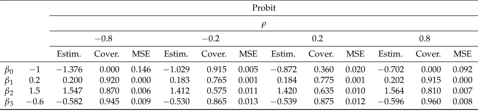
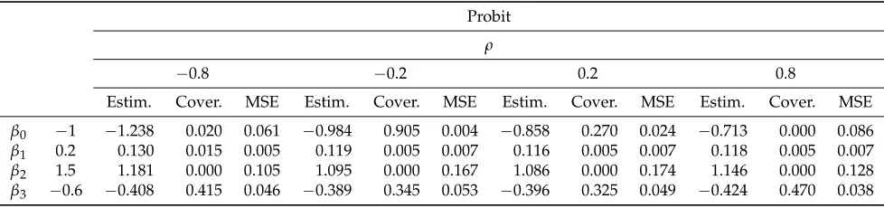
Table 4. Monte Carlo simulation results: average values of estimates, coverage of confidence intervals and MSEs. Data generating scheme:n=5000,α0 =0.05;

α1=0.20,ρ∈ {±0.2;±0.8}; censored observations approximately 30%.

Probit

ρ

−0.8 −0.2 0.2 0.8

β0 −1 −1.238 0.020 0.061 −0.984 0.905 0.004 −0.858 0.270 0.024 −0.713 0.000 0.086

β1 0.2 0.130 0.015 0.005 0.119 0.005 0.007 0.116 0.005 0.007 0.118 0.005 0.007

β2 1.5 1.181 0.000 0.105 1.095 0.000 0.167 1.086 0.000 0.174 1.146 0.000 0.128

(12)

Table 4.Cont.

SS

ρ

−0.8 −0.2 0.2 0.8

θ0 0.5 0.498 0.940 0.001 0.502 0.910 0.001 0.499 0.895 0.001 0.499 0.875 0.001

θ1 0.8 0.795 0.895 0.001 0.803 0.930 0.001 0.797 0.875 0.001 0.801 0.880 0.001

θ2 −0.5 −0.500 0.915 0.001 −0.504 0.925 0.001 −0.506 0.915 0.001 −0.507 0.820 0.001

β0 −1 −0.923 0.690 0.018 −0.939 0.710 0.015 −0.886 0.570 0.022 −0.865 0.420 0.028

β1 0.2 0.124 0.000 0.006 0.119 0.005 0.007 0.117 0.010 0.007 0.111 0.000 0.008

β2 1.5 1.094 0.000 0.174 1.085 0.000 0.177 1.072 0.000 0.187 1.076 0.005 0.189

β3 −0.6 −0.410 0.400 0.050 −0.363 0.305 0.072 −0.430 0.465 0.044 −0.448 0.445 0.043

ρ (*) −0.553 0.105 0.068 −0.124 0.790 0.014 0.109 0.760 0.019 0.495 0.110 0.108

MIS

ρ

−0.8 −0.2 0.2 0.8

α0 0.05 0.046 0.880 0.000 0.052 0.790 0.001 0.055 0.750 0.002 0.058 0.670 0.002

α1 0.2 0.190 0.845 0.007 0.194 0.865 0.006 0.200 0.905 0.005 0.197 0.905 0.003

β0 −1 −1.517 0.360 0.319 −1.144 0.935 0.068 −0.975 0.855 0.044 −0.798 0.720 0.082

β1 0.2 0.229 0.935 0.004 0.211 0.900 0.003 0.215 0.920 0.003 0.236 0.945 0.004

β2 1.5 1.711 0.910 0.135 1.569 0.890 0.088 1.587 0.920 0.094 1.742 0.940 0.149

(13)

Table 4.Cont.

MIS-SS

ρ

−0.8 −0.2 0.2 0.8

α0 0.05 0.043 0.720 0.121 0.047 0.580 0.121 0.037 0.595 0.121 0.037 0.470 0.121

α1 0.2 0.195 0.720 0.036 0.230 0.790 0.035 0.172 0.705 0.037 0.173 0.720 0.037

θ0 0.5 0.501 0.915 0.001 0.501 0.900 0.001 0.503 0.900 0.001 0.501 0.945 0.001

θ1 0.8 0.805 0.950 0.001 0.803 0.935 0.001 0.803 0.940 0.001 0.802 0.925 0.001

θ2 −0.5 −0.502 0.930 0.001 −0.502 0.945 0.001 −0.503 0.915 0.001 −0.504 0.930 0.001

β0 −1 −1.035 0.865 0.046 −0.959 0.780 0.054 −0.968 0.800 0.043 −0.970 0.760 0.032

β1 0.2 0.198 0.810 0.002 0.209 0.870 0.003 0.189 0.740 0.003 0.192 0.735 0.002

β2 1.5 1.493 0.780 0.044 1.574 0.825 0.092 1.480 0.725 0.251 1.478 0.720 0.114

β3 −0.6 −0.527 0.810 0.052 −0.609 0.845 0.066 −0.562 0.860 0.033 −0.574 0.880 0.045

ρ (*) −0.729 0.825 0.023 −0.235 0.940 0.034 0.179 0.905 0.020 0.714 0.815 0.024

(14)

4. Application on Real Data: Estimating the Effect of Tax Morale on Undeclared Work in Southern European Countries

According to EU definition, undeclared work is any paid activities that are lawful as regard their nature, but not declared to the public authorities. It is therefore referable as a special form of tax evasion, perpetrated by the employers. Tax compliance decisions have always been of great interest to researchers and policy makers. In a seminal work ofAllingham and Sandmo(1972), tax evasion is modeled as a portfolio choice made by a rational individual: he/she maximizes the expected utility of the tax evasion gamble, weighing the benefits of a successful cheating against the costs arising from detection and punishment. In this light, deterrence policies are seen as the key elements to increase tax compliance.

The main shortcoming of the Allingham and Sadmo model is that it predicts a much higher tax evasion level than that actually observed in real economic systems (Torgler 2001b;Torgler 2001a). The high levels of tax compliance registered around the world suggested that there are factors other than the economic ones (e.g., audit probabilities, tax rates, penalty rates, and income) that matter as much if not more. Hence, tax morale has emerged as one important determinant of tax behavior. The term “tax morale” was introduced bySchmölders(1960) back in 1960 who defined it as “the attitude of a group or the whole population of taxpayers regarding the question of accomplishment or neglect of their tax duties; it is anchored in citizens’ tax mentality and in their consciousness to be citizens, which is the base of their inner acceptance of tax duties and acknowledgment of the sovereignty of the state”.

Despite the definition of Schmölders, tax morale is still a debated concept with different meanings. Some authors (Braithwaite and Ahmed 2005;Feld and Frey 2002) perceive it as the “internalized obligation to pay tax”, while others (Alm and Torgler 2006) as the “intrinsic motivation” to pay taxes.

One of the most used methods to elicit tax morale is through surveys. Respondents are presented with compliant/non-compliant situations whose acceptability have to be assessed according to their system of beliefs. It is the case of the Eurobarometer survey No. 402 conducted in 2013 to unravel the attitudes of European citizens towards and their involvement in undeclared activities. We downsized the original sample of 27,563 adults aged 15 years or older to those living in one of the seven southern European countries (Portugal, Malta, Italy, Spain, Cyprus, Greece and Croatia). The size of the sub-sample is 6039 units. Interviews were either administered face-to-face or as CAPI (computer assisted personal interview).

To assess the effect of different tax moral dimensions, we used a statistical model whose observed dependent variable assumes value 1 if the interviewed answered yes to the question “Apart from a regular employment, have you yourself carried out any undeclared paid activities in the last 12 months?”, and 0 otherwise. The set of controls of the outcome equation were identified in accordance to the existing literature (Williams and Horodnic 2015a;Williams and Horodnic 2015b;Williams and Horodnic 2017). These include:

• Female: A dummy variable with value 1 for women and 0 for men.

• Age: A quantitative variable indicating the age of the respondent when interviewed.

• Urban: A dummy variable with value 1 if the respondent lives in a town of any size, and 0 otherwise.

• Children: A quantitative variable indicating the number of children less than 10 years old living in the household.

• Occupation: A categorical variable that states if the respondent is either unemployed, self-employed, employed, retired or inactive.

• Financial problems: A categorical variable grouping individuals by their difficulties in paying bills. The values are “most of the time”, “from time to time” and “almost never/never”.

(15)

• Detection risk: A categorical variable stating if the individual perceives a very high, fairly high, fairly small or very small probability of being detected when perpetrating fraudulent behavior. • Expected sanction: A categorical variable with three levels corresponding to what the individual

believes the sanction would be if caught in fraudulent behavior. The levels are: “Tax or social security contributions”, “Tax or social security contributions plus a fine”, and “Prison”.

• Tax moral: A set of three continuous variables each capturing one specific dimension of the general concept.

To be more specific regarding tax morale, we considered the following three dimensions: (1) business-level macro behaviors (TM1); (2) individual-level micro behaviors (TM2); and (3) explicit fraudulent behavior (TM3).

Each oh these dimensions is measured aggregating several corresponding elementary indicators through the arithmetic mean (in this way, we assume that the elementary indicators used for each dimension are substitutable; seeNardo et al.(2008)). In particular, TM1 considers the interviewed opinions on the following situations: “A firm is hired by a private household for work and it does not report the payment received in return to tax or social security institutions”, “A firm is hired by another firm for work and it does not report its activity to tax or social security institutions”, and “A firm hires a private person and all or a part of the salary paid to him/her is not officially registered”. TM2 is computed from the statements: “Someone uses public transport without a valid ticket” and “A private person is hired by a private household for work and he/she does not report the payment received in return to tax or social security institutions although it should be reported”. TM3 averages the opinions about “Someone receives welfare payments without entitlement” and “Someone evades taxes by not or only partially declaring income”. Each statement scores on a 10-point Likert scale, where 1 means that the behavior is absolutely unacceptable and 10 means absolutely acceptable. Consequently, by construction, each hypothesized dimension ranges itself from 1 to 10 and the lower is the index, the higher is the tax morale.

The first source of bias comes from the censoring due to non-responses on the dependent variable (around 5% of the interviewed refused to answer the question about their involvement in paid undeclared activities) and the second is about the concrete possibility that people actually employed off-the-book are reluctant to admit it and could have answered “No, I’m not employed off-the-book” when in fact they are.

At the same time, we believe unlikely the opposite kind of misclassification (that is, a person not employed off-the-book answering yes), thus we expect a very low value (if not zero) for the probabilityα0.

If we would ignore the censoring mechanism and the fact thatα0 andα1 might be nonzero, the probability of observing an off-the-book worker (see Equation (11)) would be wrongly estimated. In such a situation, the reference model is a simple probit.

To cope with censoring, we specified a selection equation considering all the covariates that may influence non-response. Some covariates are in common with the outcome equation but one is included only in the selection equation. This latter variable is thethe respondent cooperation, which is a four-level score the interviewer uses to asses the respondent’s willingness to cooperate during the interview2, whereas the ones in common are female, age, tax-morale, detection risk and country.

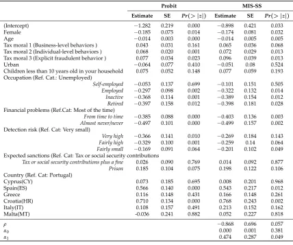
We present in Table5the results from a probit model and the model described in Section2. First, we can note that the two models produce coherent estimates, consistent with other findings in the literature3_{, according to which the typical individual involved in undeclared work activities is a young}

2 _{The variable “respondent cooperation” guarantees that the model is identified even if the assumption of normality does not}

hold, because it makesX16=X2.

3 _{The association between tax morale and the participation in undeclared activities is well known in the literature and was}

(16)

unemployed male, who has financial difficulties in paying the household bills most of the time, lives in an urban area, has a very low perception of detection risk, his/her expected sanction for a fraudulent behavior is prison and there are no kids in the household. Now, however, not all the estimates are statistically significant. This is the case of urban area, presence of kids, detection risk (for model MIS-SS only we obtained weak significance), and expected sanctions.

Referring to tax morale, coherently with our expectations, in both models, the probability of participation in undeclared work decreases as the level of morality increases. However, we may observe that tax morale variables could be endogenous, since unobservables affecting the propensity to be an undeclared worker also affect the level of tax morale indicators. Nonetheless, this problem goes far beyond the scope of the present work and we intend to address it in the future. In the context of the southern countries, however, the most significant drivers are the two dimensions related to individual level behavior. It is important to underline that tax morale variables could be endogenous, since unobservables affecting the propensity to be an undeclared worker also affect the level of tax morale indicators. Nonetheless, this problem goes far beyond the scope of the present work and we intend to address it in the future.

Referring to country effect, it emerges that almost all the southern countries are similar with respect to the behaviors on undeclared activities; the only exceptions are Croatia and Spain, where the probability of undeclared work becomes higher.

Some final considerations refer to the supplementary parameters of MIS-SS specification, which allow managing not only the problem of the bias arising from the presence of missing data in the dependent variable, but also the problem of its misclassification. In fact, as already observed, it is reasonable to think that respondents could be somewhat reticent in declaring themselves as undeclared workers and, consequently, there is a lack in measuring the prevalence of the phenomenon.

In particular, coherently with our expectations of very low or zero probability that a non-undeclared worker answer to be undeclared,α0estimates are approximately zero. On the contrary,α1estimates are very high (although not highly significant) and this result confirms that there is a share of population that declares to have not worked off-the-book when in fact they did, also consistently with expectations.

As is known, in applied problems, a useful tool to evaluate model performance is the confusion matrix, which allows the computation of percent correct prediction. Unfortunately, when the data are misclassified, the measure is unreliable. However, in our application, this is partially true. In fact, as the estimatedα0 is roughly zero, it follows thatP(TYi = 1|obsYi = 1,Xi) ≈ 1, and therefore it makes sense to compare the percent correct predictions that a worker is undeclared, under the two models. As shown in Figure1, no matter the cutoff, the percent correct predictions from MIS-SS always dominates probit.

(17)

Figure 1.Percent correct predictions of undeclared workers.

Table 5.Estimates of the drivers of participation in undeclared activities.

Probit MIS-SS

Estimate SE Pr(>|z|) Estimate SE Pr(>|z|)

(Intercept) −1.282 0.219 0.000 −0.898 0.421 0.033

Female −0.185 0.075 0.014 −0.174 0.081 0.032

Age −0.014 0.003 0.000 −0.014 0.005 0.005

Tax moral 1 (Business-level behaviors ) 0.043 0.031 0.161 0.065 0.036 0.068 Tax moral 2 (Individual-level behaviors ) 0.068 0.020 0.001 0.072 0.029 0.013 Tax moral 3 (Explicit fraudulent behavior ) 0.077 0.034 0.023 0.096 0.039 0.013

Urban −0.064 0.077 0.410 −0.051 0.08 0.524

Children less than 10 years old in your household 0.075 0.052 0.148 0.077 0.059 0.193 Occupation (Ref. Cat.: Unemployed)

Self-employed −0.053 0.137 0.699 −0.101 0.151 0.505 Employed −0.297 0.098 0.002 −0.322 0.132 0.014 Inactive −0.368 0.114 0.001 −0.389 0.154 0.012 Retired −0.397 0.158 0.012 −0.398 0.181 0.028 Financial problems (Ref.Cat: Most of the time)

From time to time −0.385 0.088 0.000 −0.403 0.136 0.003 Almost never/never −0.497 0.101 0.000 −0.499 0.157 0.002 Detection risk (Ref. Cat: Very small)

Very high −0.366 0.141 0.010 −0.269 0.184 0.143 Fairly high −0.329 0.100 0.001 −0.259 0.14 0.064 Fairly small −0.169 0.091 0.064 −0.201 0.102 0.049 Expected sanctions (Ref. Cat: Tax or social security contributions

Tax or social security contributions plus a fine 0.026 0.090 0.769 0.014 0.092 0.877 Prison 0.185 0.104 0.075 0.198 0.122 0.106 Country (Ref. Cat: Portugal)

Cyprus(CY) 0.073 0.185 0.695 0.008 0.201 0.968

Spain(ES) 0.566 0.140 0.000 0.543 0.217 0.012

Greece 0.116 0.148 0.431 0.166 0.148 0.261

Croatia(HR) 0.710 0.134 0.000 0.768 0.243 0.002

Italy(IT) 0.108 0.157 0.491 0.213 0.152 0.162

Malta(MT) -0.036 0.241 0.882 0.052 0.227 0.818

ρ −0.868 0.696 0.057

α0 0.000 0.001 0.381

α1 0.474 0.287 0.049

5. Conclusions

(18)

A simulation study highlighted that the performances of the point estimators are very satisfactory compared to the existing estimators that allow managing each problem at a time, or to the benchmark probit model. Actually, parameter estimates from our model outperform both those from sample selection model and those from Hausman et al.’s (Hausman et al. 1998) proposal.

The results obtained in an empirical analysis referring to undeclared work give strength to our proposal. Actually, even if it is impossible to assess the global goodness of fit in presence of misclassified data, in our application, we could compare the percent correct predictions for undeclared workers. Our model clearly outperforms probit. Another point that adds strength to our proposal is that, for all covariates included in the model, we obtained parameter estimates coherent with the existing literature.

Future research will be devoted, first, to disentangling the effects coming from the two sources of bias, verifying the existence of a possible offsetting. Secondly, we will extend MIS-SS model by introducing a misclassification problem in the selection equation as well. A third extension could be the specification of the misclassification probabilities as a function of some covariates. Another interesting direction for future research could refer to the problems arising from measurement errors in the covariates of the outcome equation, which currently is well known for intrinsically introducing an endogeneity issue.

Author Contributions:The authors contributed equally to the work.

Funding:Sapienza University, grant number 00041_19_RDB_ATENEO2018_AREZZO.

Conflicts of Interest:Authors declare no conflict of interest.

References

Abrevaya, Jason, and Jerry A. Hausman. 1999. Semiparametric estimation with mismeasured dependent variables: An application to duration models for unemployment spells. Annals of Economics and Statistics243–75. [CrossRef]

Allingham, Michael, and Agnar Sandmo. 1972. Income tax evasion: A theoretical analysis. Journal of Public Economics1: 323–38. [CrossRef]

Alm, James, and Benno Torgler. 2006. Culture differences and tax morale in the united states and in europe.

Journal of Economic Psychology27: 224–46. [CrossRef]

Braithwaite, Valerie, and Eliza Ahmed. 2005. A threat to tax morale: The case of australian higher education policy.Journal of Economic Psychology25: 523–40. [CrossRef]

Cameron, A. Colin, and Pravin K. Trivedi. 2005. Microeconometrics: Methods and Applications. New York: Cambridge University Press.

Chua, Tin Chiu, and Wayne A. Fuller. 1987. A model for multinomial response error applied to labor flows.

Journal of the American Statistical Association82: 46–51. [CrossRef]

Dubin, Jeffrey A., and Douglas Rivers. 1989. Selection bias in linear regression, logit and probit models.Sociological Methods & Research18: 360–90.

Feld, Lars P., and Bruno S. Frey. 2002. Trust breeds trust: How taxpayers and treated. Economics of Governance

2: 87–99. [CrossRef]

Hausman, Jerry A., Jason Abrevaya, and Fiona M. Scott-Morton. 1998. Misclassification of the dependent variable in a discrete-response setting. Journal of Econometrics87: 239–69. [CrossRef]

Heckman, James J. 1979. Sample selection bias as a specification error. Econometrica 47: 153–62. [CrossRef] Hug, Simon. 2010. The effect of misclassifications in probit models: Monte carlo simulations and applications.

Political Analysis18: 78–102. [CrossRef] [CrossRef]

Katz, Jonathan N., and Gabriel Katz. 2010. Correcting for survey misreports using auxiliary information with an application to estimating turnout. American Journal of Political Science54: 815–35. [CrossRef]

Lee, Lung-Fei. 2007. Self-Selection. InA Companion to Theoretical Econometrics. Edited by Badi H. Baltagi. Oxford: Blackwell Publishing Ltd., Chapter 18, pp. 383–409.

(19)

Mellow, Wesley, and Hal Sider. 1983. Accuracy of response in labor market surveys: Evidence and implications.

Journal of Labor Economics1: 331–44. [CrossRef]

Nardo, M., M. Saisana, A. Saltelli, S. Tarontola, A. Hoffman, and Enrico Giovannini. 2008.Handbook on Constructing Composite Indicators: Methodology and User Guide. Paris: OECD.

Poterba, James, and Lawrence Summers. 1995. Unemployment benefits and labor market transitions: A multinomial logit model with errors in classification.The Review of Economics and Statistics77: 207–16. [CrossRef] Schmölders, Gunter. 1960. Das Irrationale in der öffentlichen Finanzwirtschaft: Probleme der Finanzpsychologie.

Rowohlts Deutsche Enzyklopädie: Staats- und Wirtschaftswissenschaften. Rowohlt.

Sullivan, Paul. 2009. Estimation of an occupational choice model when occupations are misclassified. The Journal of Human Resources44: 495–535. [CrossRef]

Torgler, Benno. 2001a. Is tax evasion never justifiable? Journal of Public Finance and Public Choice20: 143–68. Torgler, Benno. 2001b. What do we know about tax morale and tax compliance? International Review of Economics

and Business48: 395–419.

Vella, Francis. 1998. Estimating models with sample selection bias: A survey. The Journal of Human Resources33: 127–69. [CrossRef]

Williams, Colin C., and Ioana A. Horodnic. 2017. Evaluating the policy approaches for tackling undeclared work in the european union. Environment and Planning C: Politics and Space35: 916–36. [CrossRef]

Williams, Colin C., and Ioana A. Horodnic. 2015a. Evaluating the prevalence of the undeclared economy in central and eastern europe: An institutional asymmetry perspective.European Journal of Industrial Relations

21: 389–406. [CrossRef]

Williams, Colin C., and Ioana A. Horodnic. 2015b. Rethinking the marginalisation thesis: An evaluation of the socio-spatial variations in undeclared work in the european union.Employee Relations37: 48–65. [CrossRef]

c