Ecm parameters for generating surface having low coefficient of friction in lubricated condition by using genetic algorithm

(1)

ECM PARAMETERS FOR GENERATING SURFACE HAVING LOW COEFFICIENT OF FRICTION IN

LUBRICATED CONDITION BY USING GENETIC ALGORITHM

Siddhartha

Department of Manufacturing Engineering,

A R T I C L E I N F O

INTRODUCTION

The ability to machine very complex features in hard and difficult to machine materials with negligible tool wear, reasonable accuracy and acceptable surface finish has made electrochemical machining (ECM) an

traditional machining process. Many process parameters both controllable and uncontrollable determine the material removal rate, accuracy and surface texture. [1-6]. Statistical design has been used extensively to model the effect of

parameters of ECM on output parameters such as surface roughness, material removal rate (MRR), overcut [5,7

Maximizing one output parameter usually affects another desirable output parameter. A variety of approaches such as goal programming [11], Particle swarm optimization [12 Desirability Approach [15, 16], Genetic algorithm has been employed to find a set of optimal solutions involving conflicting objective functions [7-9, 17]. In this paper a set of non-dominated solutions i.e. Pareto front is obtained using multi objective genetic algorithm. However, choosing a representative solution from a set of non-dominated solution is not easy. Clustering solutions in Pareto front has been used by many authors [18-20]. One common method of choosing the representative solution is to select the non dominated solution which is nearest to the cluster centroid [20].

Functional performance of engineering components in service is strongly influenced by surface roughness.

International Journal of Current Advanced Research

ISSN: O: 2319-6475, ISSN: P: 2319-6505,

Available Online at www.journalijcar.org

Volume 7; Issue 4(A); April 2018; Page No.

DOI: http://dx.doi.org/10.24327/ijcar.2018

which permits unrestricted use, distribution, and reproduction in any medium, provided the original work is properly cited.

Article History:

Received 24th January, 2018 Received in revised form 13th

February, 2018 Accepted 8th_{March, 2018} Published online 28th April, 2018

Key words:

Electrochemical Machining, SG Iron, Surface roughness, Multi-objective Genetic algorithm, Cluster analysis.

*Corresponding author: Siddhartha Karmakar

Department of Manufacturing Engineering, NIFFT, Hatia, Ranchi, India

ECM PARAMETERS FOR GENERATING SURFACE HAVING LOW COEFFICIENT OF FRICTION IN

LUBRICATED CONDITION BY USING GENETIC ALGORITHM

**Siddhartha Karmakar* and Mandal A**

of Manufacturing Engineering, NIFFT, Hatia, Ranchi, India

A B S T R A C T

Coefficient of friction in service is strongly influenced by surface roughness parameters. The objective of this work is to maximize the surface roughness parameters S minimize Sq, SHTp, Ssk to lower the coefficient of friction in lubricated case.

genetic algorithm is used to find the Pareto front consisting of a number of non dominated solutions. The number of solutions found is large. Agglomerative hierarchical clustering method is used to obtain 3,4 and 5 clusters. Two linkage metho

are used to generate clusters with population 45 and 100. The Pareto optimal points closest to the cluster centroids are obtained. Complete linkage, population 45, cross over:0.8 represents the population well. The cluster1 and cluster 2 (complete linkage, population 45, cross over:0.8) which have low values of Sq and Shtp

high value of Sku and a low value of Ssk.

The ability to machine very complex features in hard and difficult to machine materials with negligible tool wear, reasonable accuracy and acceptable surface finish has made important non-any process parameters both controllable and uncontrollable determine the material removal 6]. Statistical design has been used extensively to model the effect of different process parameters of ECM on output parameters such as surface roughness, material removal rate (MRR), overcut [5,7-10] etc. Maximizing one output parameter usually affects another desirable output parameter. A variety of approaches such as programming [11], Particle swarm optimization [12-14], Desirability Approach [15, 16], Genetic algorithm has been employed to find a set of optimal solutions involving 9, 17]. In this paper a set of ns i.e. Pareto front is obtained using multi objective genetic algorithm. However, choosing a dominated solution is not easy. Clustering solutions in Pareto front has been used by ethod of choosing the representative solution is to select the non dominated solution

Functional performance of engineering components in service

A single surface texture parameter is not sufficient to reflect true quality of the product [21].

necessary to characterize the functional property of a surface. For example friction and wear has been reported to be influenced by surface roughness parameters such as (R (Rt,Rz), Rsk, Rku, RDelA,Wa [21]. Wear is reported [22] to be larger when the initial values of the amplitude parameters S Sq and SHtp as well as rms. slope S

[23] that in case of dry wear test, coefficient of friction is low when roughness is high. In lubricated case, when roughness is low, then coefficient of friction is low. It is reported [23] that increase in parameter Rku led to decrease in friction in lubricated case and increase in friction for dry tests. Friction also observed to be lower when t

more negative in lubricated tests.

Based on the above reports it is decided to locate optimal process parameters for ECM namely applied potential, inter electrode gap and machining time for low coefficient of friction for lubricated condition.

Objective

The objective function for lubricated case Ssk and Maximize Sku

METHODOLOGY

The first step is to develop mathematical models to predict the effect of process variables on surface roughness parameters Sq, Ssk, Sku, SHTp. To use the models to calculate the values of roughness parameters at any point in the allowable design space.

International Journal of Current Advanced Research

6505, Impact Factor: 6.614

www.journalijcar.org

; Page No. 11318-11322

//dx.doi.org/10.24327/ijcar.2018.11322.1956

and Mandal A. This is an open access article distributed under the Creative Commons Attribution License, which permits unrestricted use, distribution, and reproduction in any medium, provided the original work is properly cited.

Karmakar

Department of Manufacturing Engineering, NIFFT, Hatia,

ECM PARAMETERS FOR GENERATING SURFACE HAVING LOW COEFFICIENT OF FRICTION IN

LUBRICATED CONDITION BY USING GENETIC ALGORITHM

Ranchi, India

oefficient of friction in service is strongly influenced by surface roughness parameters. The objective of this work is to maximize the surface roughness parameters Sku and to lower the coefficient of friction in lubricated case. Multi objective genetic algorithm is used to find the Pareto front consisting of a number of non dominated solutions. The number of solutions found is large. Agglomerative hierarchical clustering method is used to obtain 3,4 and 5 clusters. Two linkage methods- centroid and complete are used to generate clusters with population 45 and 100. The Pareto optimal points closest to the cluster centroids are obtained. Complete linkage, population 45, cross over:0.8

luster 2 (complete linkage, population 45, can be further analyzed to select a

A single surface texture parameter is not sufficient to reflect true quality of the product [21]. Combination of parameters is the functional property of a surface. For example friction and wear has been reported to be influenced by surface roughness parameters such as (Ra, Rq), [21]. Wear is reported [22] to be larger when the initial values of the amplitude parameters Sk, as well as rms. slope SDq are high. It is reported [23] that in case of dry wear test, coefficient of friction is low lubricated case, when roughness is low, then coefficient of friction is low. It is reported [23] that led to decrease in friction in lubricated case and increase in friction for dry tests. Friction also observed to be lower when the parameter Rsk tends to be more negative in lubricated tests.

Based on the above reports it is decided to locate optimal process parameters for ECM namely applied potential, inter-electrode gap and machining time for low coefficient of

icated condition.

The objective function for lubricated case- Minimize Sq ,SHTp,

The first step is to develop mathematical models to predict the effect of process variables on surface roughness parameters- . To use the models to calculate the values of roughness parameters at any point in the allowable design

Research Article

(2)

The second step is to use these models to generate optimum levels of process parameters (Pareto front) for minimum coefficient of friction for lubricated condition using multi objective genetic algorithm in MATLAB environment.

The third step is to use clustering methods for obtaining representative solutions from the large number of solutions in the Pareto front.

Experiment Details

The experimental work and mathematical models used in this work are reported in ref.16. The essential details are presented here.

The matrix selected for conducting the experiments is eighteen points face centered composite design. The actual and coded values of the different variables are listed in Table-1. The design matrix is shown in Table-2.

Table 1 ECM process Variables and Their Levels

Variables Symbol Low level Medium level High level

Actual Coded Actual Coded Actual Coded

VOLTAGE(volt) V 15 -1 20 0 25 +1

TIME(min) T 2 -1 3 0 4 +1

GAP(mm) G 0.64 -1 0.96 0 1.28 +1

Table 2 Design matrix of three process parameter for surface roughness

SL NO Voltage Machining time Inter electrode gap

1 -1 -1 -1

2 1 -1 -1

3 -1 1 -1

4 1 1 -1

5 -1 -1 1

6 1 -1 1

7 -1 1 1

8 1 1 1

9 -1 0 0

10 1 0 0

11 0 -1 0

12 0 1 0

13 0 0 -1

14 0 0 1

15 0 0 0

16 0 0 0

17 0 0 0

18 0 0 0

ECM machine model ECMAC - II, manufactured by MetaTech Industries, Pune, is used with a round shaped tool made of copper. Electrolyte used is a mixture of NaCl and NaNO3 solution (125 grams of NaCl and 250 grams of NaNO3 / litre of tap water). Work piece material selected is SG Iron 450/12 grade received courtesy M/s. Hindustan Malleables & Forging Ltd., Dhanbad, India. The chemical composition of the material is given in Table3.The material has pearlitic matrix. Hardness (Brinell)-196.

Table 3 Chemical Composition of SG Iron 450 grades. [45]

C Si Mn P S Cr Mo Cu Mg Ti

3.365 2.393 0.238 0.072 < 0.150 0.0072 < 0.010 0.37 0.085 0.032 Zn Fe Others(Bi,Ce,Co,La,W,V,Ta,Sn,B,As,Zr,Sb,etc..)

0.027 90.75 2.6608

Developing the Models

To analyze the effects of the process variables on the surface roughness parameters such as Sq, Ssk, Sku, SHtp, the following second order polynomial is used.

Y = Bo + B1T+ B2V +B3G+ B11T2 + B22V2 +B33G2 +B12TV+B13TG+B23VG . . . (1)

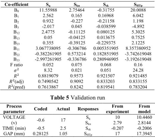
Where, B's are the regression coefficients. V, T, G are the controllable process parameters in coded form. To check the adequacy of the statistical regression models analysis of variance are carried out. F-ratios of the models developed are calculated and are compared with the corresponding tabulated values for 95% level of confidence. The goodness of fit of the models are tested by calculating R2, R2(adjusted) & R2(predicted) . Design Expert [24] is used to develop the models. The coefficients of the models developed and the model statistics for the models are given in Table-4. All the models are statistically adequate. To validate the models further one set of experiment are carried out at levels different than those of design matrix (table 5).

Table 4 The Coefficients for surface roughness parameter

Co-efficient Sq Sku Ssk SHTp

B0 11.55988 2.75464 -0.31755 20.0088

B1 2.562 0.165 0.16968 6.042

B2 0.932 -0.227 -0.21158 1.198

B3 -2.017 0.045 -0.038599 -4.892

B12 2.4775 -0.11125 0.080125 5.3025

B13 0.05 -0.04125 0.013675 0.7525

B23 0.355 -0.39125 -0.229375 2.1225

B11 3.067738095 -0.306786 0.005351905 8.357380952

B22 -0.382261905 0.573214 0.182851905 -3.742619048

B33 -2.997261905 -0.336786 0.280946905 -3.192619048

F ratio 0.052 0.075 0.068 0.16 8.32 0.021 0.051 24.28 0.8819079 0.9573 0.921507 0.921485 (adj) 0.7490542 0.9092 0.833203 0.833155 (pred) 0.7613867 0.8242 0.819541 0.783204

Table 5 Validation run

Process

parameter Coded Actual Responses

From experiment

From model

VOLTAGE

(v) -0.6 17

Sq 10 10.4460

Sku 2.79 2.8144

TIME (min) -0.5 2.5 Ssk -0.207 -0.2006

GAP (mm) 0.28125 1.05 SHTp 17 17.3945

For locating optimum levels of process parameters for minimum coefficient of friction for lubricated condition genetic algorithm, a multi objective optimization technique is used. The four objective functions for lubricated case Sq, Sku, Ssk, SHTp are constructed using the coefficients given in table 4.

Table 6 Upper and lower limit of surface parameters In the design space

Surface Roughness

Parameter Lower Limit Upper Limit

Sq 5.35 20.434

Sku 1.8267 3.747

Ssk -0.6612 0.675

SHTp 4.795 37.687

(3)

clusters. In this paper a standard agglomerative hierarchical clustering technique with centroid method and complete linkage method are used. The numbers of clusters considered are 3, 4 and 5. The Pareto optimal point closest to the cluster centroid is obtained and given in tables 7-15.

RESULTS AND DISCUSSIONS

Table 7 3 clusters with centroid linkage (population 45, cross over function 0.8)

Number of observations

Within cluster sum

of squares

Average distance from centroid

Maximum distance

from centroid

Cluster1 15 2.8396 0.397144 0.84417 Cluster2 49 14.6352 0.498108 1.05384 Cluster3 16 1.6856 0.291102 0.56894

Pareto optimal point closest to cluster centroid.

of squares

Cluster1 14 2.0761 0.354904 0.77007 Cluster2 49 14.6352 0.498108 1.05384 Cluster3 16 1.6856 0.291102 0.56894 Cluster4 1 0.0000 0.000000 0.00000

Pareto optimal point closest to cluster centroid

Number of

observations

of squares

Cluster1 13 1.4375 0.311919 0.58616 Cluster2 49 14.6352 0.498108 1.05384 Cluster3 16 1.6856 0.291102 0.56894 Cluster4 1 0.0000 0.000000 0.00000 Cluster5 1 0.0000 0.000000 0.00000

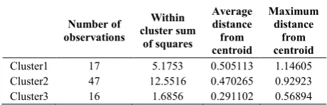
Table 10 3 clusters with complete linkage (population 45, cross over function 0.8)

of squares

Cluster1 33 5.1650 0.370557 0.617876 Cluster2 103 23.7100 0.455306 0.823288 Cluster3 29 2.4490 0.256935 0.755899 Cluster4 10 0.8512 0.262023 0.492615 Cluster V T G Sq Sku Ssk Shtp

Cluster1 -0.97526 0.938669 0.870361 6.470658 2.19516 -0.60856 9.456993 Cluster 2 0.128561 -0.75225 0.711175 7.647237 3.34388 0.197843 11.23132 Cluster 3 0.08798 0.971285 -0.10921 12.71175 3.11053 -0.29697 18.95483 Cluster 4 -0.9266 -0.03025 0.999725 6.791637 2.10105 -0.2249 12.85199

Cluster V T G Sq Sku Ssk Shtp

Cluster1 -0.97526 0.938669 0.870361 6.470658 2.19516 -0.60856 9.456993

Cluster 2 0.128561 -0.75225 0.711175 7.647237 3.34388 0.197843 11.23132

Cluster 3 0.08798 0.971285 -0.10921 12.71175 3.11053 -0.29697 18.95483

Cluster1 -0.97526 0.938669 0.870361 6.470658 2.19516 -0.60856 9.456993

Cluster 2 0.128561 -0.75225 0.711175 7.647237 3.34388 0.197843 11.23132

Cluster 3 0.08798 0.971285 -0.10921 12.71175 3.11053 -0.29697 18.95483

Cluster 4 -0.16134 0.668552 0.998909 6.634894 2.29074 -0.32676 11.03159

Cluster 5 -0.9266 -0.03025 0.999725 6.791637 2.10105 -0.2249 12.85199

Cluster1 -0.99804 0.76007 0.998912 5.880925 1.98035 -0.54353 9.818269 Cluster 2 0.224842 -0.92998 0.775492 6.961643 3.61368 0.365856 9.216878 Cluster 3 0.08798 0.971285 -0.10921 12.71175 3.11053 -0.29697 18.95483

Cluster1 -0.99804 0.76007 0.998912 5.880925 1.98035 -0.54353 9.818269

Cluster 2 0.224842 -0.92998 0.775492 6.961643 3.61368 0.365856 9.216878 Cluster 3 0.08798 0.971285 -0.10921 12.71175 3.11053 -0.29697 18.95483

Cluster 4 0.38848 -0.65294 0.376625 10.35341 3.25261 0.028677 17.18728

Cluster1 -0.97526 0.938669 0.870361 6.470658 2.19516 -0.60856 9.456993 Cluster 2 0.224842 -0.92998 0.775492 6.961643 3.61368 0.365856 9.216878 Cluster 3 0.08798 0.971285 -0.10921 12.71175 3.11053 -0.29697 18.95483 Cluster 4 0.38848 -0.65294 0.376625 10.35341 3.25261 0.028677 17.18728

Cluster 5 -0.60973 -0.15337 0.55063 9.151852 2.54744 -0.29607 15.56235

Cluster1 -0.51223 0.932189 0.800339 7.116287 2.47455 -0.50733 9.754073

Cluster 2 0.251945 -0.8292 0.600708 8.384413 3.47648 0.204483 12.35301

(4)

of squares

Table 16 3 cluster with complete linkage (population 45, cross over function 0.6)

of squares

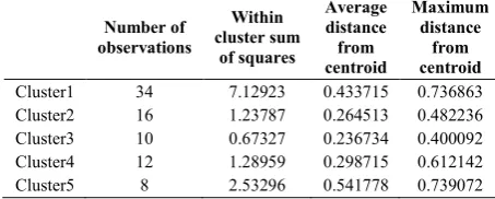
Table18 5 clusters with complete linkage (population 45, cross over function 0.6)

of squares

When the centroid and complete linkage are compared two interesting trends are observed Table (9 &12). The cluster 1 and 3 are same. Second cluster in centroid case which contains 49 elements are shown as two clusters (29 elements and 18 elements) in complete linkage. Centroid linkage (table 9) has two clusters having 1 element each. The Pareto optimal point closest to the centroids for clusters 4 &5 (table 9) are quite close. Where as in case of complete linkage the Pareto optimal point closest to the centroids are well dispersed (table 12). When population is increased to 100 little change in Pareto optimal points closest to the centroids are observed when compared to the results obtained with population of 45 (table 12 &15). Effect of changing the cross over function from 0.8 to 0.6 is studied also (table 12 & 18). The trends observed are similar. If Sku and Ssk are considered then it is observed that is Ssk is in the range -0.6 to -0.6 then Sku is in the range 2.2-2.3. If Sku is in the range 3.37-3.6 the Ssk is in the range .03-0.36. Sq and Shtp show similar trends. As Sq decreases Shtp decreases. It seems the case: complete linkage, population 45, cross over:0.8 (Table 12) represents the population well. The cluster1 and cluster 2 (complete linkage, population 45, cross over:0.8) which have low values of Sq and Shtp can be further analyzed to select a high value of Sku and a low value of Ssk.

CONCLUSIONS

The objective of this work is to minimize the surface roughness parameters Sq, SHTp , Ssk and maximize Sku to lower the coefficient of friction in lubricated case. Multi objective genetic algorithm is used to find the Pareto front consisting of a number of non dominated solutions. The number of solutions found is large. Agglomerative hierarchical clustering method is used to obtain a number of clusters. Representative solutions are selected by choosing the non dominated solution which is nearest to the cluster centroid. Complete linkage, population 45, cross over:0.8 represents the population well. The cluster1 and cluster 2 (complete linkage, population 45, cross over:0.8 ) which have low values of Sq and Shtp can be further analyzed to select a high value of Sku and a low value of Ssk.

Roughness Parameters

All parameters with S is 3D extension of R roughness profile parameter: for example Sq is the 3D extension of Rq

RDelA : Average Slope of the Profile. Rt : Maximum Height of Profile.

Sa: Arithmetic Mean Deviation of the Surface, µm SDq : Root mean square gradient of the surface SHtp: Surface section height difference (20% - 80%) Sku: Kurtosis of the Topography Height Distribution. Sq: Root-Mean-Square (RMS) Deviation of the Surface,µm Sp: Surface section height difference (20% - 80%)

Ssk: Skewness of the Topography Height Distribution. Sz: Ten Point Height of the Surface,µm.

Wa : MeanValue of the Waviness of the Unfiltered Profile.

Experimental Variables

T : Time of machining (minutes)

Cluster1 -0.74002 0.936349 0.748625 7.196147 2.42517 -0.57331 9.89996

Cluster 2 0.251945 -0.8292 0.600708 8.384413 3.47648 0.204483 12.35301

Cluster 3 -0.02138 0.963365 -0.17742 12.20159 3.11469 -0.30201 17.86244

Cluster 4 -0.31038 -0.05957 0.942502 6.451072 2.46465 -0.1329 11.16594

Cluster1 -0.74002 0.936349 0.748625 7.196147 2.42517 -0.57331 9.89996 Cluster 2 0.034209 -0.86372 0.897901 5.986445 3.45794 0.375203 7.652399 Cluster 3 0.349626 -0.77345 0.158849 10.77425 3.36783 0.023694 17.46678 Cluster 4 -0.02138 0.963365 -0.17742 12.20159 3.11469 -0.30201 17.86244 Cluster 5 -0.31038 -0.05957 0.942502 6.451072 2.46465 -0.1329 11.16594

Cluster1 0.409319 -0.99062 0.662845 7.946185 3.73084 0.361523 11.03765

Cluster 2 -0.9981 0.990087 0.753339 7.1653 2.31339 -0.642 10.1014

Cluster 3 0.058386 0.992969 -0.11689 12.56536 3.13239 -0.2979 18.47358

Cluster1 0.161251 -0.98672 0.995853 5.044897 3.66168 0.551765 5.528087

Cluster 2 -0.9981 0.990087 0.753339 7.1653 2.31339 -0.642 10.1014

Cluster 3 0.562784 -0.83927 -0.06411 11.88601 3.37332 0.038957 20.29753 Cluster 4 0.058386 0.992969 -0.11689 12.56536 3.13239 -0.2979 18.47358

Cluster1 0.409319 -0.99062 0.662845 7.946185 3.73084 0.361523 11.03765

Cluster 2 -0.9981 0.990087 0.753339 7.1653 2.31339 -0.642 10.1014

(5)

V : Applied potential(volts) G : Inter electrode gap(mm)

References

1. McGeough J.A, Principles of Electrochemical Machining, Chapman and Hall, 1974

2. Rumyantsev E, and Davydov A, Electrochemical Machining of Metals, Mir Publishers Moscow, 1989, 13- -36.

3. Krishnaiah Chetty O.V, Murthy, R.V.G.K and Radhakrishnan V, On Some Aspects of Surface Formation in ECM, Trans. ASME, J. Engg. Ind.,

1981,Vol. 103, 341-348.

4. Sorkhel S.K. and Bhattacharyya B., Parameter Control by Optimal Quality of the Workpiece Surface in ECM,

J. Materials Processing Technology,1994,vol.40, 271-286.

5. Bhattacharyya B. and Sorkhel S.K., Investigation for controlled Electrochemical Machining Through Response Surface Methodology, J. Materials Processing Technology, 1999, Vo.86, 200-2007. 6. João Cirilo da Silva Neto , Evaldo Malaquias da Silva ,

Marcio Bacci da Silva. Intervening Variables in Electrochemical Machining. Journal of Materials Processing Technology, 2006, Vol.179,pp. 92-96. 7. Senthilkumar C,Ganesan G. and Karthikeyan r.,

Optimizaion of ECM Process Using NSGA-II, Journal of Minerals and Materials Characterization and Engineering, 2012, vol. 11,931-937.

8. Giribabu A., Rama Rao S. and Padmanbhan G., Optimization of Machining Parameters in ECM of Al/B4C Composites using Genetic Algorithm, Int. J. Mech. Eng. & Rob. Res., 2014, vol.3, no.3, 32-38. 9. Sathyammoorthy V.,Sekar T. and Elango N.,

Optimization of Processing Parameters in ECM of Die Tool Steel Using Nanofluid by Multiobjective Genetic Algorithm, The Scientific World Journal, Volume 2015, Article ID 895696, 6 pages, 2015. doi:10.1155/2015/895696

10. Kunal Kamal, B.M.Jha and A.Mandal, Effect of Electrolyte Concentration on Material Removal Rate and Overcut during Machining of SG Iron, Int. J. Scientific Progress and Research, Vol.22, no.3, 2016,127132.

11. Acharya B.G., Jain V.K. and Batra J.L., Multi-objective Optimization of ECM Process, Precision Engineering, 1986, vol.8, issue 2, 88-96.

12. Rao R.V., Pawar P.J. and Shankar R., Multi-objective Optimization of Electrochemical Machining Process Parameters Using A Particle Swarm Optimization Algorithm, Proc. I.MechE., vol 222, Part B:J. Engineering Manufacture, 949-958.

13. Chenthil Jegan T.M. and Ravindran d., Electrochemical machining Process Parameter Optimization using Particle Swarm Optimization, Computational Intelligence, 2017, vol.33, issue 4, 1019-1037.

14. Bhandari S. and Shukla N., Parametric Optimization of Electrochemical Machining By Particle Swarm Optimization Technique, SSRG Int. J. Mechanical Engineering(SSRG-IJME) 2015, vol.21, issue 5, 23-19. 15. Derringer G, Suich R., Simultaneous Optimization of

Several Response Variables, J. Quality Technology, 1980, vol,12, no.4 (October), 214-219.

16. Siddharta Karmakar and Amitava Mandal, Multicriteria Optimization of Surface Roughness Produced in Electrochemical Machining using Mixed Electrolyte NaNO3 and NaCl, Int. J. Modern Engineering Research, vol.6, issue 7, 2016,41-49.

17. Jain, N.K. and Jain V.k., Optimization of Electrochemical Machining Process Parameters Using Genetic Algorithm, Machining Sci. Technol., 2007, 11,235-258.

18. Morse J., Reducing the size of the nondominated set: Purning by Clustering, Computers & Operations Research, Vol.7, 1980, 55-66.

19. Roseman M.A. and Gero J.S., Reducing the Pareto Optimal Optimal set in Multicriteria Optimization,

Engineering Optimization, 1985, Vol.8, 189.

20. Chaudhari P.M., Dharaskar R.V. and Thakare V.M., Computing the Most Significant Solution from Pareto Front Obtained in Multi-objective Evolutionary, (IJACSA) Int. J. Adv. Computer Science and Applications, 2010, vol.1, no.4, October, 63-68.

21. Petropoulus G.P, Pandazaras C.N, Paulo Davim J, Surface Texture Characterization and Evaluation Related to Machining, in Surface Integrity in Machining, Ed. Paulo Davim J, Springer, 2010, 37-66. 22. Grabon W, Pawlus P, Sep J, Tribological

Characteristics of One-Process and Two-Process Cylinder Liner Honed Surfaces Under Reciprocating Sliding Conditions, Tribology International, 2010, vol.43,1882-1892.

23. Sedlaček M, Podgornik B,Vižintin, Influence of Surface Preparation on Roughness Parameters, Friction and Wear, Wear, 2009, vol.266, 482-487.

24. Design-Expert V9®-product of M/s Stat-Ease Inc. 25. Matlab , The Math Works Inc., Natick, MA, USA 26. Minitab 18-product of Minitab Inc.

*******

How to cite this article: