Manuscript Title & Authors

(1)

e-ISSN: 2278-7461, p-ISSN: 2319-6491

Volume 7, Issue 7 [July 2018] PP: 01-15

Assessment of the Impact of automobile Waste on the

Environment

Ogundapo Tayo

1

, Tobinson. A. Briggs

2

1_{Department of Environmental Engineering,University of Port Harcourt, Rivers State,} 2_{Department of}_Mechatronic_{Engineering, University of Port Harcourt, Nigeria}

Corresponding Authur, Tobinson. A. Briggs

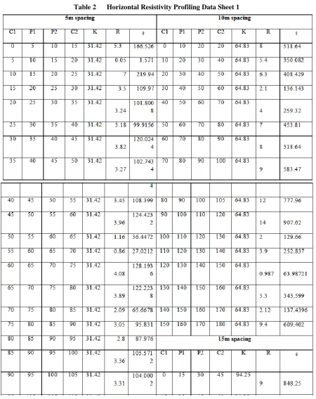
ABSTRACT : This study is on automobile waste penetration, the depth and thickness of the contaminated area by the use of vertical electrical sounding and horizontal resistivity profiling. Schlumberger and Wenner array was employed in the resistivity sounding and profiling, using an Abem SAS 300B terrameter. In this survey, electrodes were arranged in a straight line with constant spacing and connected to multicore cables. The field survey was conducted along four profiles which provide a continuous coverage of electrical sounding and profiling. The surface soil material is mainly sands. The result showed that profile line 4(Vertical Electrical Sounding I) has the highest depth of automobile wastes penetration which is about 60m while profile line 3 (Vertical Electrical Sounding 3) has the least depth of automobile wastes penetration which is about 0.4m. Also, profile line 3 has the highest thickness of the contaminated area which is about 14m while profile line 4, has the least thickness of contaminated area which is about 5m. The result of this work could serve as a baseline study for future evaluation of automobile wastes, when allocating site to Automobile workshop.

KEYWORDS: automobile waste, electrical sounding, waste penetration, resistivity, profiling, automobile workshop

--- --- Date of Submission: 28-06-2018 Date of acceptance: 13-07-2018 --- ---

I. INTRODUCTION

Automobile waste such as used lubricating oil, used grease, contaminated petrol and diesel, acid and calcium carbide are generated from Auto-mechanic workshops that repair and service auto-mobiles. These wastes are not properly disposed of, since there is hardly any stipulated law regulating their locations, activities and operations.

These workshops create and discharge automobile wastes into our environment (soil) some of which add dirty or harmful substances to air so that it is no longer pleasant or safe to use. These wastes are possible and available sources of environmental pollution if not properly get rid of and managed.

The common method used by the users of these wastes and operators of automobile workshops to get rid of these wastes is by pouring them on the ground which either penetrate into the soil or washed by rainstorm into drains. When used lubricating oil is poured down drains or onto the ground, the oil is not water down. Oil that is not properly getting rid of will find its way into the soil.

The result of this study will provide information about the lateral extent and vertical depth of penetration of used lubricating oil, contaminated petrol/diesel and used grease and their relationship with existing borehole (hydraulic head). This information could serve as a baseline study for future evaluation of automobile and polycylic aromatic hydrocarbons (PAHS) pollution in Elekhia (Nigeria) mechanic village soils and providing allocation for automobile workshop. Although there are varieties of waste generated in a workshop, the automobile wastes to be study in this work are used lubricating oil, contaminated petrol and diesel used grease, acid and calcium carbide. The field base physical parameters of the existing bore-hole (hydraulic head) such as colour, odour and taste were study.

II. METHODOLOGY 2.1 Sources of Data:

(2)

MN is the distance between the potential electrodes π = 3.142 or

Apparent resistivity (е) such that

е = K X R……….………… 2

Where R is resistance read on the MiniRes

Table.1: Vertical Electrical Sounding 1, 2 and 3 Data Sheet for Profile Line One

AB/2 MN/2 K VES 1

R1

ᵨ1 VES 2

R2

ᵨ2 VES 3

R3

ᵨ3

1 0.25 0.9375 3.5 3.28125 4.56 4.275 1.05 0.9843

1.5 0.25 2.1875 5.84 12.775 7.65 16.7343 2.031 4.4428

2 0.25 100.14 10.42 1043.459 11.32 1133.585 3.042 304.6259

3 0.25 225.80 15.93 3596.994 14.42 3256.036 5.04 1138.032

4 0.5 200.28 21.12 4229.914 17.41 3486.875 4.03 807.1284

4 0.25 401.73 32.01 12859.38 22.41 9002.769 3.05 1225.277

5 0.5 313.37 25.12 7871.854 28.6 8962.382 2.08 651.8096

6 0.5 451.60 17.73 8006.868 30.32 13692.51 1.091 492.6956

8 0.5 803.46 11.21 9006.787 20.23 16254 0.921 739.9867

10 1 626.75 8.23 5158.153 16.12 10103.21 0.682 427.4435

10 0.5 1255.85 6.23 7823.946 8.32 10448.67 0.461 578.9469

15 1 1412.15 4.231 5974.807 4.45 6284.068 0.234 330.4431

20 1 2511.70 2.02 5073.634 2.03 5098.751 0.172 432.0124

30 1 5653.30 0.93 5257.569 0.54 3052.782 0.0984 556.2847

40 2.5 4017.31 0.321 1289.557 0.094 377.6271 0.0704 282.8186

40 1 10051.53 0.023 231.1852 0.0085 85.43801 0.058 582.9887

50 2.5 6279.26 0.342 2147.507 0.0043 27.00082 0.045 282.5667

60 2.5 9043.86 0.001 9.04386 0.0023 20.80088 0.0321 290.3079

80 2.5 16081.03 0.0034 54.6755 0.0011 17.68913 0.0065 104.5267

100 10 6267.48 0.0067 41.99212 0.0321 201.1861 0.0043 26.95016

100 2.5 25128.81 0.0065 163.3373 0.0043 108.0539 0.0032 80.41219

150 10 14121.46 0.076 1073.231 0.0045 63.54657 0.0016 22.59434

200 10 25117.03 0.0078 195.9128 0.041 1029.798 0.0012 30.14044

2.4 Geometric factor and apparent resistivity

The generalized formula for calculating geometric factor (Kg) for a four-electrode configuration is:

Kg = 2π ( ) -1 ……….…….. .3

(3)

(4)

2.5 Methods of Data Analysis

The vertical electrical sounding (VES) data were used to determine the possible depth of automobile waste penetration while the Horizontal resistivity profiling (HRP) data were used to determine the possible plumes and lateral extent that is the thickness of the contaminated area. Vertical Electrical Sounding (VES) data were inputted to the computer and curves were plotted using 1X1D version 3.44 interpretation software as shown in figure1 to figure 12.

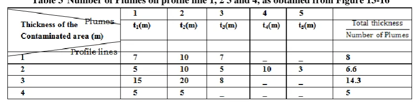
2.6 Total Thickness of Contaminated Area

(5)

Where, is the arithmetic mean and the divisor n is the total number of items so added. The subscript i go from 1 to n and indicate the position of each observation in the set.

Table 3 Number of Plumes on profile line 1, 2 3 and 4, as obtained fromFigure 13-16

III. RESULTS AND DISCUSSION 3.1 Presentation of Data

Graph of depth plotted against resistivity and apparent resistivity plotted against spacing obtained from vertical electrical sounding data are presented in Figure 1 to figure 12. The essence of the data and plots is to show the variation of contaminant level with depth and lithology level with depth.

3.2 Data Analysis of Vertical Electrical Sounding

At profile line I (Vertical Electrical Sounding 1), the possible depth of wastes penetration and the inferred lithology were 27m and sands respectively as shown in table 1. This implies that the soil of profile line 1 (Vertical Electrical Sounding 2) is severely polluted with this automobile wastes.

At profile line 1 (Vertical Electrical Sounding 2), the possible depth of wastes penetration and the inferred lithology were 6m and gravels respectively as shown in table 2. This implies that the soil of profile line 1 (Vertical Electrical Sounding 2) is moderately polluted with this automobile wastes.

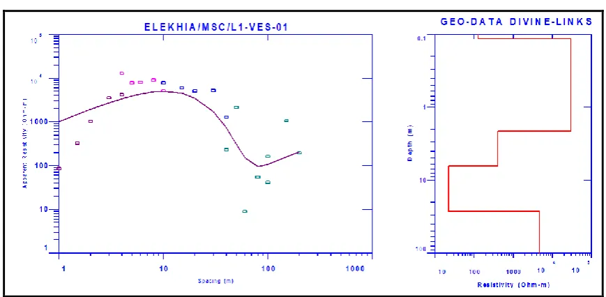
At profile line 1 (Vertical Electrical Sounding 3), the possible depth of wastes penetration and the inferred lithology were 22m and sands respectively as shown in table 3. This implies that the soil of profile line 1 (Vertical Electrical Sounding 3) is severely polluted with this automobile wastes.

At profile line 2 (Vertical Electrical Sounding 1), the possible depth of wastes penetration and the inferred lithology were 11m and sands respectively as shown in table 4. This implies that the soil of profile line 2 (Vertical Electrical Sounding 1) is severely polluted with this automobile wastes.

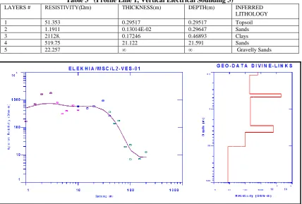
At profile line 2 (Vertical Electrical Sounding 2), the possible depth of wastes penetration and the inferred lithology were 4m and sandy clays respectively as shown in table 5. This implies that the soil of profile line 2 (Vertical Electrical Sounding 2) is moderately polluted with this automobile wastes.

At profile line 2 (Vertical Electrical Sounding 3), the possible depth of wastes penetration and the inferred lithology were 12m and sandy clays respectively as shown in table 6. This implies that the soil of profile line 2 (Vertical Electrical Sounding 3) is severely polluted with this automobile wastes.

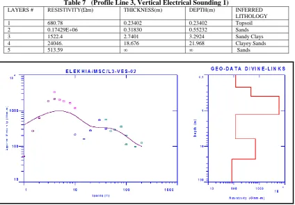
At profile line 3 (Vertical Electrical Sounding 1), the possible depth of waste penetration and the inferred lithology were 1m and sands respectively as shown in table 7. This implies that the soil of profile line 3 (Vertical Electrical Sounding 1) is slightly polluted with this automobile wastes.

At profile line 3 (Vertical Electrical Sounding 2), the possible depth of wastes penetration and the inferred lithology were 6m and sandy respectively as shown in table 8. This implies that the soil of profile line 3, (Vertical Electrical Sounding 2) is moderately polluted with this automobile wastes.

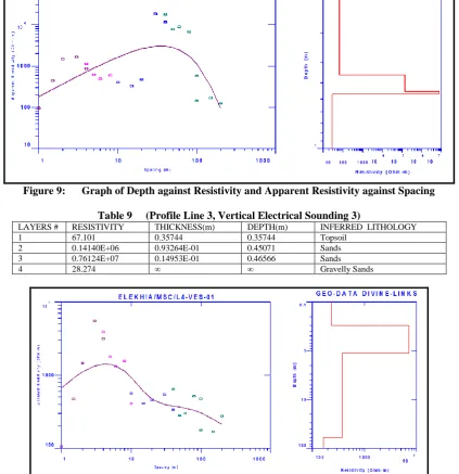
At profile line 3 (Vertical Electrical Sounding 3), the possible depth of waste penetration and inferred lithology were 0.4m and sands respectively as shown in table 9. This implies that the soil of profile line 3, (Vertical Electrical Sounding 3) is slightly polluted with this automobile wastes.

At profile line 4 (Vertical Electrical Sounding 1), the possible depth of wastes penetration and the inferred lithology were 60m and sandy clays as shown in table 10. This implies that the soil of profile line 4, (Vertical Electrical Sounding 1) is severely polluted with this automobile wastes.

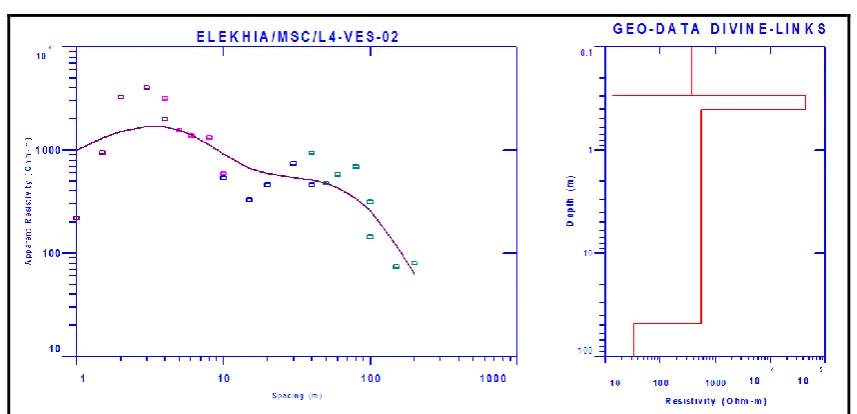
At profile line 4 (Vertical Electrical Sounding 2), the possible depth of wastes penetration and inferred lithology were 48m and sands respectively as shown in table11. This implies that the soil of profile line 4, (Vertical Electrical Sounding 2) is severely polluted with this automobile wastes.

(6)

Figure 1: Graph of Depth against Resistivity and Apparent Resistivity against Spacing

Table 1 (Profile Line 1, Vertical Electrical Sounding 1)

LAYERS # RESISTIVITY(Ώm) THICKNESS(m) DEPTH(m) INFERRED

LITHOLOGY

1 126.03 0.11604 0.11604 Topsoil

2 29816. 1.9895 2.1055 Clays

3 404.99 4.2299 6.3354 Sandy Clays

4 22.560 20.269 26.605 Sands

5 4654.9 ∞ ∞ Clayey Sands

LAYERS # RESISTIVITY(Ώm) THICKNESS(m) DEPTH(m) INFERRED LITHOLOGY

1 19.638 0.13149E-01 0.13149E-01 Topsoil

2 26852. 1.8665 1.8797 Clays

3 3.1491 4.0183 5.8980 Sandy gravels

(7)

LITHOLOGY

1 51.353 0.29517 0.29517 Topsoil

2 1.1911 0.13014E-02 0.29647 Sands

3 21128. 0.17246 0.46893 Clays

4 519.75 21.122 21.591 Sands

5 22.257 ∞ ∞ Gravelly Sands

1 660.77 0.11830 0.11830 Topsoil

2 194.00 0.27285 0.39115 Clayey Sands

3 19420. 0.83807E-01 0.47496 Clays

4 214.68 2.3842 2.8592 Sandy Clays

5 6318.9 1.5259 4.3851 Silty Clays

6 98.320 6.3106 10.696 Sands

(8)

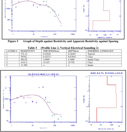
Figure 5 Graph of Depth against Resistivity and Apparent Resistivity against Spacing

LAYERS # RESISTIVITY THICKNESS(m) DEPTH(m) INFERRED LITHOLOGY

1 531.12 0.24444 0.24444 Topsoil

2 58702. 0.43372 0.67816 Clays

3 682.82 3.6909 4.3690 Sandy Clays

4 4141.4 15.423 19.792 Clays

5 31.590 ∞ ∞ Sands

1 411.28 0.38300 0.38300 Topsoil

2 2580.4 1.1566 1.5396 Clays

3 2867.1 10.141 11.681 Sandy Clays

(9)

LITHOLOGY

1 680.78 0.23402 0.23402 Topsoil

2 0.17429E+06 0.31830 0.55232 Sands

3 1522.4 2.7401 3.2924 Sandy Clays

4 24046. 18.676 21.968 Clayey Sands

5 513.59 ∞ ∞ Sands

LAYERS # RESISTIVITY THICKNESS(m) DEPTH(m) INFERRED

LITHOLOGY

1 117.61 0.22245 0.22245 Topsoil

2 469.06 0.17477 0.39722 Sandy Clay

3 5911.0 0.87523 1.2725 Sandy Clays

4 115.12 4.9087 6.1812 Sands

5 704.70 16.516 22.697 Silty Sands

(10)

1 67.101 0.35744 0.35744 Topsoil

2 0.14140E+06 0.93264E-01 0.45071 Sands

3 0.76124E+07 0.14953E-01 0.46566 Sands

1 232.02 0.30104 0.30104 Topsoil

2 7124.5 0.81109 1.1121 Clays

3 376.00 59.235 60.347 Sandy Clays

(11)

1 373.56 0.29467 0.29467 Topsoil

2 13.586 0.80105E-03 0.29547 Sand

3 43609. 0.11381 0.40928 Clays

4 555.08 47.761 48.170 Sands

1 105.74 0.26525 0.26525 Topsoil

2 353.48 0.20240 0.46765 Sandy Clays

3 6301.7 2.1378 2.6055 Clays

4 1116.1 16.749 19.354 Clayey Sands

5 105.64 ∞ ∞ Sands

3.3 Data Analysis of Horizontal Resistivity Profiling

(12)

(13)

Figure14: Horizontal Resistivity Profiling 2 (NUMBER OF PLUMES)

(14)

Figure16: Horizontal Resistivity Profiling 4 (NUMBER OF PLUMES)

IV. ORGANOLYPTICTEST

Organolyptic test was carried out to find out the field base physical parameters of the existing borehole (hydraulic head) in the workshop. It was found that the water from the borehole has odour, colour and has a taste. This implies that the water is not suitable for consumption.

V. CONCLUSION

(15)

[5]. Forstner U. Calmano W. Hong J. Kersten M. (1998). Effects of redox variations on metal speciation. Waste Manage. Res. 4:95-104 [6]. Gilber U.A, Oladele O. (2009). Assessment of soil-pollution by slag from an automobile battery manufacturing plant in Nigeria.

Afr. J. Environ Sci. Tech. 3(9): 239-250

[7]. Horsfall M. Jr (2001). Advanced Environmental Chemistry 1st_{Ed. Lalimesters Printer Port-Harcourt, Nigeria. PP. 130-159}

[8]. Maynard B.J, Turer D.G (2003). Heavy metal contamination in highway soils. Clean Tech. Environ on. Policy 4: 235-245 [9]. Mbah CN, Ezeaku P.I (2010). Physicohemical Characterization of farmland affected by Automobile wastes in relation to Heavy

Metal Nature. Sci. 8(10).

[10]. Mbah CN, Anikwe MAN (2010). Variation in Heavy metal contents on roadside soils along a major express way in South east Nigeria NY. Sci. J.3 (10).

[11]. Nick B., Katerina K. (2011). Application of half schlumberger configuration for detecting Karstic cavities and voids for a wind farm site in Greece. Journal of Earth Science and Geotechnical Engineering Vol. no.1, 2011, 101 – 116

[12]. Nwachukwu M.A, Ntesat B. and Mbaneme F.C (2013). Assessment of Direct Soil Pollution in Automobile Junk Market. Journal of Environmental Chemistry and Ecotoxicology. Vol. 5(5). PP.136 – 146

[13]. Nwachukwu MA, Feng H, Achilike K. (2010b). Integrated study for automobile wastes management and environmentally friendly mechanic villages in the Imo River Basin Nigeria; Afri. J. Environ. Sci. Tech 4(4): 234 – 249

[14]. Nwachukwu MA, Feng H, Alinnor J (2010a). Assessment of heavy metals pollution in soil and their implications within and around mechanic villages, Int. J. Env. Sci. Tech. 7(2): 347-358

[15]. Ololade, I.A; Lajide, L. and Amoo, I.A. (2007) Enrichment of Heavy Metals in sediments as pollution indictor of the aquatic ecosystem. Pakistan Journal of scientific and industrial Research, 50, 27-35 [Citation Time(s):1]

[16]. Ololade, I.A (2014). An Assessment of Heavy-Metal contamination in soils within Auto-Mechanic Workshops using enrichment and contamination factors with Geoaccumulation Indexes. Journal of Environmental Protection Vol.5 No. 11 (2014), Article ID: 49118.

[17]. Oyegun CU. (1999). The Port – Harcourt Region, university of Port-Harcourt Press Limited. P.195.

[18]. Sucharova J., Suchara I., Hola M., Marikova S. Rermann C., Boyd R., Filzmoser P. and Engimaier P. (2012). Top /bottom Soil ratios and Enrichment Factors: what do they really show? Applied Geochemistry, 27, 138-145. http://dx.doi.org/10.1016/j.apgeochem.2011.09.025 [citation Time(s): 3]

[19]. Zeinab A., Abdulrahim S., Wan Z.Y. and Jasni Y. (2012). Groundwater investigation using electrical resistivity imaging technique. Bulletin of the Geological society of Malaysia, Volume 58, Pp.55-58.