Abstract— Monte Carlo (MC) simulation is extensively used for solving thermal radiation problems in high-temperature environments, such as combustion chambers and furnaces, and irregular-geometry enclosures containing participative media such as combustive gases. The quantities of interest are surface radiosities and subsequent radiative heat fluxes which have been accurately determined by MC in configurations which are challenging for deterministic formulations. The attractiveness of MC schemes becomes more prominent in mixed-mode and coupled thermo-fluid problems, where the non-linearity, spectral characteristics and geometrical complexity may render deterministic treatments largely ineffective. This work deals with thermal radiative estimates for hot grey diffuse surfaces and grey participative media. S imple test-configurations are considered for which exact solutions are available and MC simulation is used to make validation comparisons. We also consider the analog simulation process to compute sensitivities of independent parameter variations, such as material density, in a single simulation. S uch a capability increases the applicability of MC methods to optimization studies as easily as deterministic methods based on variational schemes.
Index Term— Mixed-mode heat transfer, Monte Carlo simulation, participating media, S tochastic sensitivity, Thermal radiation.
I. INT RODUCT ION
MONTE CARLO (MC) simulation has been extensively used for solving thermal radiation problems in high -temperature environments including combustion chambers and furnaces, and irregular-geometry enclosures containing participative media such as combustive gases. Surface radiosities and subsequent heat fluxes have been accurately determined in configurations which are difficult for deterministic formulations. The attractiveness of MC schemes becomes more prominent in mixed-mode and coupled thermo-fluid
Dr. Zafar Ullah Koreshi is a Professor at Air University, Islamabad, Pakistan (Ph: 0092(345)5115936; fax: 0092(51)9260158; e -mail:
zafar@ mail.au.edu.pk.)
Engr. Sadaf Siddiq is an Assistant Professor at Air University, Islamabad, Pakistan. (Ph: 0092(333)5637932; fax: 0092(51)9260158 ;
e-mail: sadaf@ mail.au.edu.pk. )
Dr. T asneem M. Shah is a Professor at Air University, Islamabad, Pakistan. (Ph: 0092(300)5269610; fax: 0092(51)9260158; e -mail:
dr.tasneem@ mail.au.edu.pk.)
problems, where the non-linearity, spectral characteristics and geometrical complexity may render deterministic treatments largely ineffective.
This work deals with thermal radiative estimates for hot grey diffuse surfaces and grey participative media. Simple test-configurations are considered for which the exact solutions are available and MC simulation is used to make validation comparisons. We consider two problems viz (i) a two-surface source-sink infinite configuration, and (ii) an enclosure with fixed-temperature surfaces.
Three methods -- an electric circuit analogy model, a deterministic integral formulation, and a Monte Carlo simulation model -- are used to estimate the radiative heat flux and in some cases, the temperature distribution.
The MC simulation is based on tracking the history of bundles of photons from ‗birth‘, as emitted photons, to ‗death‘ when they are absorbed at a surface or within a participative medium. We consider the accuracy and precision of MC estimates as a function of the number of photon bundles sampled and the radiative properties of surfaces. Surface radiosities are determined from surface irradiations in scattering events. The accuracy of MC estimates, known to depend strongly on both the geometry and emissivity, is quantified for the test configurations. From this, we are able to obtain estimates of the required sample size for simulation. Similarly, the emissivity data for surfaces determines the events in a history. Strong absorption at a surface, for example, terminates a history before it makes a ‗significant‘ contribution to a tally of interest at the other surface. Such an ‗analog‘ MC simulation is bound to give significant errors and hence requires modification by one or several methods.
In the last part of the paper, we consider sensitivity capabilities of MC simulation to obtain perturbations in estimates of radiative heat flux due to independent variation in material properties. For this, improvement strategies such as artificially altering, or biasing, the underlying probability distribution function (PDF) to force more events in the simulation and ‗correct‘ the statistical tally are demonstrated to give a ‗better‘ estimate. The simplicity of the test configurations allows us to write simple terms for the probabilities of events based on the multiple scattering of photons from surfaces. We are thus able to quantify the effect of such a technique in a simulation of a simple configuration and to infer on the validity of such a scheme in complex problems. It is anticipated that this work will demonstrate ways of obtaining better MC estimates more
Monte Carlo Simulation in Thermal Radiative
Transfer: Method Review, Validation and
Parameter Sensitivity
efficiently, i.e. without excessive computational effort, and will be extended to non-grey surfaces and participative media.
II. DET ERMINIST IC AND ST OCHAST IC MET HODS
A. The Electric Circuit Analogy Method
In an elementary deterministic ―circuit diagram‖ analogy, the net heat flow can be expressed [1], [2] as
1 2 2 2 1 1 1 . 2 1
R
e
q
R
q
q
R
q
e
Q
b
b
, (1)
and an ―overall‖ flow between surface 1 and 2 can then be written as i i b b
R
e
e
Q
3 1 . 2 1
, (2)where the resistances are given by
2 2 2 3 12 1 2 1 1 1 1
1
,
1
,
1
A
R
F
A
R
A
R
. (3)Here, the view factor F12 is
Y Y X X X Y X Y Y X Y X Y X Y X xY F 1 1 2 1 2 2 1 2 2 1 2 2 2 2 tan tan ) 1 ( tan 1 1 tan 1 1 1 1 ln 2 (4)where
X
a
/
D
,
Y
b
/
D
(a, b are length and width of plates respectively and D is the distance between the plates ).B. Integral Formulation
We can also write an integral equation for the net heat flux in a gray, diffuse enclosure is [2],[3] as
' ' ' ' ) ( ) ( ) ( ) 1 ) ( 1 ( ) ( ) ( ' '
' dA dA
A b b dA dA A dF r e r e dF r q r r r q
.(5)
For two surfaces of length a, width b separated by distance D two equations can be written from Eqn.(5). For coordinates x1
and x2 are taken along the surfaces and using
2 3 2 1 2 2 2 1 2 2 1
]
)
(
[
2
1 2 2 1x
x
D
dx
dx
D
dF
dx
dF
dx
dx dx dx dx
, the differential view factors can be found. The thermal flux equations, for isothermal surfaces, are then:
2 2 1 2 / 0 2 2 1 1
1
(
)
1
1
(
)
(
,
)
d
f
q
q
a D
(6.a)
e
be
b a Df
d
/ 0 2 2 1 2 , 1 ,(
,
)
and
/ 1 1 2 10 1 1
2 2
2
(
)
1
1
(
)
(
,
)
d
f
q
q
a D(6.b)
b a Db
e
f
d
e
/ 0 1 2 1 1 , 2 ,(
,
)
forD
x
and
2
3/21 2 2 1
)
(
1
2
1
)
,
(
f
.Consider now the integral formulation for a participating non -scattering medium between parallel plates. The integro-differential equation is [3]
I
S
(
,
s
ˆ
)
d
dI
q
(7)where the source term is given by
i i i b
q
s
w
I
I
s
s
s
d
S
(
ˆ
)
(
ˆ
,
ˆ
)
4
)
1
(
)
ˆ
,
(
4 ,
. (7.a)If the source function is known, equation (7) can be integrated and the intensity can be found as
0 ' ) ( ' ')
ˆ
,
(
)
0
(
)
(
I
e
S
s
e
d
I
(8)where
' is the optical coordinate. We consider the simple cases of two infinite plane surfaces with a non -scattering participating medium. We assume that collisions in the participating medium are all absorptions and an absorption results in a blackbody emission [2]. Writing the angular dependence explicitly, equation (8) is
I
t
tI
bt
t
t
dt
t
I
0 ' ' ')
exp(
)
(
)
/
exp(
)
,
0
(
)
,
(
(9) and separating the forward and backward components of theintensity
I
(
t
,
0
)
andI
(
t
,
0
)
we can write the radiosities from surface 1 and surface 2 as
2 0 2 / 01
cos
d
I
(
,
)
d
I
(
0
)
q
, (10.a)and
2 0 2 /2
cos
d
I
(
,
)
d
I
(
t
L)
q
. (10.b)The above quantities can be used to find the forward and
backward intensities in the medium
I
(
t
,
)
and)
,
(
t
I
respectively. From these, the forward and backwardfluxes
q
(
t
)
andq
(
t
)
respectively can be found, and thenet flux
q
(
t
)
q
(
t
)
q
(
t
)
. From the steady-state energy equation, for conduction of thermal radiation, we know thatdq
/
dt
0
. Using Leibnitz‘s Rule and relationships for exponential integral functions
1 0 2)
/
exp(
)
(
t
t
d
and defining non-dimensional quantities for the temperature field and the radiative heat flux as
2 1
2
*
(
)
q
q
q
t
e
e
bb and
2 1 *
q
q
q
q
,the resulting equations are:
L
t b
b
E
t
e
t
E
t
t
dt
e
0
' ' 1 ' * 2
*
|)
(|
)
(
)
(
2
, (11.a)and
Lt
b
t
E
t
dt
e
q
0
' ' 2 ' * *
)
(
)
(
2
1
. (11.b)The quantities above,
e
b*andq
*can be found by solving theintegral equations (11); however to find the unknowns,
e
b(
t
)
and
q
require that the surface radiosities are known. If the surface temperatures only are known, then the radiosity terms have to be replaced by the known quantities. This is achieved from the relations. The final results are then:
)
2
1
1
(
1
1
)
(
)
(
2 1 *
*
2 2 *
2 , 1 ,
2 ,
q
q
t
e
e
e
e
t
e
bb b
b b
, (12)
and
*
2 2
1 1
2 , 1 , *
1
1
1
)
(
q
e
e
q
q
b b
. (13)C. Monte Carlo Simulation
We now consider a simulation method based on following the photons as they travel from birth to their final destination. The Monte Carlo (MC) simulation [2],[5] consists of sampling ―source‖ bundles from one surface and transporting them to their final destination using laws of probability. A simulation of N histories involves the following steps for a history
i. Specification of the source emissive power. ii. Selection of emission angles θ and φ. iii. Ray tracing in the direction of propagation. iv. Determination of point of intersection, if any
with the destination surface.
v. Determination of fate of history at the destination surface.
The vector of propagation
^
S
is related to the unit vectors2 1
,
t
t
and
n
. In the direction^
S
, the point of intersection Q can be found as follows: The sample size is determinedfrom the emitted energy of a surface,
4
T
A
e
A
E
b
Watts. One selects N bundles, each bundle having energy ω such thatE
N
. In case of twosurfaces, the energy per bundle can be kept constant so that
2 2 2 1 1 1
N
E
N
E
.With surface 1 as the ―reference surface‖, the number of
bundles started from surfaces is kept as
(
)
1.
1 2
2
N
E
E
N
Thepoint of emission pe from a surface is determined as
min min
max
min min
max 1
)
(
)
(
y
y
y
y
x
x
x
x
e e
The polar and azimuthal angles θ and φ respectively are then determined as
sin
1(
3)
for a diffuse surface emitter, and
2
4. On intersection at Q, a scattering is chosen with probability1
and thus0
5
1
determines ascattering whereas
1
5
1
corresponds to anabsorption. In case of scattering, new angles θ φ are determined and the process continues until the history is terminated on absorption. The quantity of interest in the problem is the energy exchange or equivalently, the difference between the energy emitted from a surface and absorbed by that surface.
This can indeed be generated to an N-Surface configuration
j ij N
j i
b
q
F
q
e
q
1 1
1
1
and includes the ―self-contribution‖ Fijqqi +
which may be non-zero for a re-entrant surface. The quantities of interest are q+ and q- which are determined with ε, eb specified in the material
data. Tally counter counts are updated each time a surface absorption, or emission takes place. Since the present configuration consists of gray surfaces, a spectral index is not required.
The configuration considered in the following analysis has two black surfaces with a gray participating medium which has both absorption and scattering. The analysis leading to the expressions in the previous section for a purely absorbing medium also apply here, as scattering is taken to be an emission resulting from absorption in the participating medium. For simplicity, surface ‗2‘ is considered to be a zero temperature so that it does not emit any photons. The number of photon bundles started from surface 1 is
N
w,1and the energy per bundle is1 , 1 4 1 1
w
N
A
T
w
.The normalized heat flux
q
*is estimated from the number of photon bundles emitted from surface ‗1‘, and the number of photon bundles absorbed by each of the surfaces2 , 1 ,
,
w wS
S
as1 , 2 ,
1 ,
1 , 1 , *
w w
w w w
N
S
N
S
N
The distance to collision,
s
, is obtained from the PDF:ds
e
K
ds
s
f
(
)
t Kts ,from which, using a uniformly random number in the range (0,1) for the CDF, a distance to collision DTC, can be sampled as
)
1
ln(
1
t
K
s
.The average value of the DTC, or the mean free path
s
is then
0
1
)
(
t
K
ds
s
sf
s
.Alternately, in units of optical distance, also called the optical depth,
t
K
ts
, the mean optical path is then
t
1
.III. RESULT S
For the first validation exercise, we consider two parallel plates of dimensions 1m X 1m. The ―exact‖ radiosity vales are obtained from the circuit diagram method and compared with MC simulation. Tables Ia and Ib shows the results from both methods for different sample size in MC computations.
TABLE 1A
CASES CONSIDERED FOR COMP ARISON OF NET RADIATIVE HEAT FLUX FROM ELECTRICAL CIRCUIT ANALOGY AND MC ANALOG SIMULATION
METHODS.
Case
Nb,N1,N2 T1 T2 ε1 ε2 D
(K) (K) (m)
Set A Qnet=0
A1 10,103,103 2000 2000 1.0 1.0 1-5
A2 10,103,444 2000 2000 0.9 0.4 1-5 A3 10,103,111 2000 2000 0.9 0.1 1-5
Set B Qnet=0
B1 10,103,103 2000 2000 1.0 1.0 0.1 B2 10,103,444 2000 2000 0.9 0.4 0.5 B3 10,103,111 2000 2000 0.9 0.1 1.0
Set C Qnet= 60.2 k W, 9.48 k W, 2.61 k W
C1 10,103,7 2000 1000 0.9 0.1 1.0
C2 10,103,7 2000 1000 0.9 0.1 5.0
C3 10,103,7 2000 1000 0.9 0.1 10.
Set D Qnet=10.1 k W, 10.1 k W
D1 10,103,0 2000 500 0.9 0.1 5.0
D2 10,103,0 2000 250 0.9 0.1 5.0
D3 10,103,0 2000 125 0.9 0.1 5.0
Here,
N
b, N
1,
and
N
2are the batch size and the number of photons started from isothermal surfaces 1 and 2 at temperatures T1, T2 and emissivities
1,
2respectively. TableI.a. shows four sets of configurations (A, B, C and D) arranged in order of complexity. Set A has no net radiant transfer and touching surfaces, so that all started particles contact with the ‗other‘ surface and ensure ‗good‘ statistics. The number of photon bundles started at surface 1 (N1
)
is chosen arbitrarily whileN
2 is calculated from the condition requiring constantenrgy per bundle:
1
2 as described above. Set D is taken to be the ‗worst‘ case in which the statistics is expected to bepoor. For the configurations given in Table I.a., the radiosity of each surface is computed using the exact the expression (Eqn. 1) and the MC simulation described in Section II, and listed in Table I.b. The results for the MC estimate show the mean value along with the standard deviation.
TABLE IB
RADIOSITY COMP UTATIONS FORCASES CONSIDERED FOR COMP ARISON OF NET RADIATIVE HEAT FLUX FROM ELECTRICAL CIRCUIT ANALOGY AND
MC ANALOG SIMULATION METHODS.
Case Exact Radiosity MC Radiosity
q1 +
q2 +
q1 +
q2 +
A1 9.07e5 9.07e5 9.07e5 9.07e5
A2 9.07e5 9.07e5 9.07e5±1.11e3 8.96e5±1.5e4 A3 9.07e5 9.07e5 9.07e5±8.65e2 8.99e5±7.0e4 B1 9.07e5 9.07e5 9.07e5±8.6e0 9.07e5±1.49e1 B2 9.07e5 9.07e5 8.40e5±1.1e3 5.72e5±1.97e4 B3 9.07e5 9.07e5 8.21e5±3.3e2 2.38e5±2.47e4 C1 9.00e5 5.99e5 8.19e5±5.5e2 1.77e5±2.96e4 C2 9.06e5 1.42e5 8.16e5±4.2e1 1.45e4±9.75e3 C3 9.07e5 8.02e4 8.16e5±2.7e1 7.14e3±2.94e3 D1 9.06e5 9.41e4 8.16e5±3.6e1 7.7e3±7.35e3 D2 9.06e5 9.12e4 8.16e5±2.7e1 4.43e3±4.87e3 D3 9.06e5 9.09e4 8.16e5±3.6e1 5.14e3±5.73e3
For the integral equation without a participating medium, we convert the integrals (equations 6) to an Nth order Gaussian quadrature scheme
Ni
i i
f
t
w
d
f
1
1 2
2 1 1
1
)
,
(
)
,
(
and
Ni
i i
f
t
w
d
f
1
2 1
2 1 1
1
)
,
(
)
,
(
,using the transformation
) 1 (
2
y
h W
.The system of equations is
A
q
b
. In this second-orderGaussian quadrature scheme, the weights are
w
1
w
2
1
, and the evaluations are made at3
1
2 1
t
t
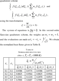
. We obtainthe normalized heat fluxes given in Table II.
TABLE II
NORMALIZED HEAT FLUXES
(W/H=1,
T
1=
T
2=1000
K
)
1
2(
)
~
4 1 1
T
q
q
ii
)
(
~
1 1
t
q
q
~
1(
t
2)
q
~
2(
t
1)
q
~
2(
t
2)
0.1 0.1 0.9388 0.9775 0.9388 0.9775 0.2 0.2 0.8825 0.9564 0.8825 0.9564 0.5 0.5 0.2341 0.1210 0.2070 0.0515 0.9 0.9 0.5900 0.8407 0.5900 0.8407touching each other with 10 batches consisting of 1000 histories from each surface, the MC results match the exact results. The standard deviations are zero in this case, as is the net heat flux. All the ―single event‖ histories consist of absorptions, no scatterings and no losses. In this sense, it is the easiest of the cases for a MC simulation. As the emissivity of the second surface decreases, the number of absorptions on this surface also decreases resulting in an increase in the error and in the standard deviation. The third run in Set A confirms the trend.
Set B is intended to quantify the error in the MC simulation due to a decrease in the view factor of the surface and hence an increase in the number of lost bundles. The accuracy of the lower emissivity surface drops due to the smaller sampled source as well as to the smaller number of absorptions on the second surface. The sharp decrease in the accuracy of the MC estimate for the third case in Set B is due to the lower emissivity of the second surface, and hence the smaller sample, and the larger loss term. In fact, out of 1111 photon bundles, the surface absorptions were 54 and 20 on surfaces 1 and 2 respectively while 1037 (93.34%) got lost. For this problem, the view factor is about 0.2 so that the about 80% of the emissions would be expected lost from the direct source.
Set C considers difficult configurations for an MC simulation in which the photon energy per bundle is kept constant. In fact, the first case of this set results in 32 and 23 absorptions on surfaces 1 and 2 respectively while 948 are lost (94%) compared with a view factor of about 0.2. The second case of this set has 0.3 and 1.2 surface absorptions respectively or 1.5% of the total while the view factor is about 1.2%. In the third case, the radiosity estimates are almost completely due to the emissions rather than from the interaction between the surfaces, which has reduced the net power exchange to only 2.61 kilowatts. Finally, Set D is the worst case for an MC simulation based on the current strategy of constant bundle energy.
The results of the deterministic integral formulation, as shown in Table II do not have any associated uncertainty other than the numerical error in the quadrature approximation but have the disadvantage that the quantities of interest are found at specific points only.
IV. APPLICAT IONS
The engineering applications of radiative flux in furnaces and 2-D and 3-D enclosures, have been obtained by MC simulations and validated experimentally, (see e.g. [4]).
The work is also extensively used for studying the effect of Thermal Barrier Coatings (TBC) which are used to reduce the heat flux on a surface so that it may perform according to the requirements. In an engine, for example, a 150 μm thick coating of yttria stabilized zirconia coating can cause a temperature drop of 170 C. Similarly, converging-diverging nozzles can be protected by similar TBCs.
The surface flux in a combustion chamber, for example, can be found here using the integral formulation with a participating medium. We consider two parallel plates of given temperatures and emissivities, separated by a non -scattering
medium. The temperature field
T
(
t
)
f
(
e
b(
T
))
between the plates and the net radiative thermal fluxq
can be determined,for which the exact results are given by equations (12) and (13). Table III shows the design requirement for cooling rate required to keep surface 2 at the prescribed temperature. This will remove the heat found as the net thermal radiative flux. Surface 1 is thus a ‗source condition‘ while surface 2 represents a sink. The engineering design problem can be to find the material corresponding to a specified absorption coefficient if plate spacing is fixed, or alternately to find the plate spacing if the material is given.
TABLE III
COOLING RATE*
(
Q
c)
REQUIRED TO KEEP SURFACE 2 AT THETEMP ERATURE
T
2K.Surface 1 Surface 2 Opt.Th. *
q
q
1
T
/K
1T
2/K
2t
K
aL
2
.
cm
W
2000 0.1 400 0.9 0 1.00 8.47
2000 0.1 400 0.9 2.5 0.34 7.52
2000 1.0 0 1.0 2.5 0.34 30.85
TABLE IV
MONTE CARLO SIMULATION ESTIMATES FOR THE NON-DIMENSIONAL
RADIATIVE HEAT FLUX
q
*Physical
s a
K
K
,
cm-1
N
w,1*
q
L,W,Z (m)
MC (MCTR.m)*
Reference Case (no scattering)
1,1,0.25 0.06,0.04 105 0.3404 0.3401
1,1,0.25 0.03,0.02 105 0.5002 0.5000
1,1,0.25 0.015,0.010 105 0.6587 0.6800
1,1,0.25 0,0 105 0.9997 1.0000
*MATLAB® program written
In the first case, the two black surfaces are at 2000 K and 0 K respectively. They have a surface area each of 1 m2and are separated by a distance 0.25 m. In the absence of a
participating medium, the net heat flow is
F
12
AT
4= 57.335W/cm2. With a participating medium
K
a
0
.
06
cm
11
04
.
0
cm
K
s , andt
L
2
.
5
,*
q
=0.34 [2] and85
.
30
4 * 1 ,
*
q
e
q
AT
Q
b
W/cm2.Notice that the view factor (0.6320 in this case) does not enter the calculation. The MC estimate with the isotropic scattering and isotropic re-emission simulation, in Table IV, gives
*
TABLE V
ACCURACY OF MONTE CARLO SIMULATION ESTIMATES FOR THE NON
-DIMENSIONAL RADIATIVE HEAT FLUX WITH THE NUMBER OF INDEP ENDENT BATCHES AND P HOTON BUNDLES SIMULATED
04
.
0
,
06
.
0
sa
K
K
CM-1S.No
B
N
N
P
*
q
q*1 10 10 4.5000e-001 1.5652e-001
2 10 100 3.3300e-001 4.1243e-002
3 10 1000 3.3710e-001 1.5764e-002
4 10 10000 3.4084e-001 4.3502e-003
5 10 100000 3.4098e-001 1.4154e-003
6 20 100000 3.4040e-001 1.4415e-003
The present analysis can be applied for such situations to determine the effectiveness of candidate TBCs. including metals, semiconductors and dielectrics which can be used.
V. MC SENSIT IVIT Y A. Material Perturbations
To study the effect of material perturbation, we consider cases in which the independent parameters
K
a,
K
sare varied. Such work has been included in MC simulation for neutrons and photons, for example, in production codes such as MORSE [6] and MCNP [7]. The theory was demonstrated by Rief [9] and extended and applied in nuclear fusion reactor design sensitivity studies (see e.g. [10],[11.In order to get some idea of the magnitude of change in the net heat flux due to a material perturbation, we carry out full re-runs when
K
aalone is varied. The MC tallies are shown in Tables VIa and VIb.TABLE VIA
MONTE CARLO SIMULATION ESTIMATES (RE-RUNS) FOR THE CHANGE IN RADIATIVE HEAT FLUX DUE TO A P ERTURBATION IN THE MATERIAL
ABSORP TION; BASE CASE
K
a
0
.
06
,
K
s
0
.
04
CM-1,(1000X10)a
K
(%)
No. of Absorptions
in M edium
No. of scatterings in M edium
t
t
/
(%)
* *
/
q
oq
(%)
-20 23815 19910 -12.0
(2.2) +8.5
-10 26764 19692 -6.0 +3.7
0 29935 19857 0 0
10 33320 20232 +6.0 -4.0
20 35866 20051 +12.0
(2.8) -7.0
TABLE VIB
MONTE CARLO SIMULATION ESTIMATES (RE-RUNS) FOR THE CHANGE IN RADIATIVE HEAT FLUX DUE TO A P ERTURBATION IN THE MATERIAL SCATTERING; BASE CASE
K
a
0
.
06
,
K
s
0
.
04
CM-1,(1000X10)s
K
(%)
No. of Absorptions
in Medium
No. of scatterings in Medium
t
t
/
(%)
*q
(%)
-20 30551 16397 -8 (2.30) +6.4
-10 29759 17979 -4 (2.40) +2.9
0 29935 19857 0 (2.50) 0
10 29526 21661 4 (2.60) -2.8
20 29138 23333 8 (2.70) -4.7
The thermal radiative transfer formulation is very similar to the neutron and photon transport as it based on the integral form of the Boltzmann equation. Traditionally, MC simulation is seen to be analogous to the Neumann series solution of the governing integral equation. Thus, we consider an idealized, extensively studied, 1-D slab transmission problem for which the exact solution is readily available (see e.g. [8]).
A simple demonstration of the perturbation method will be made by way of the slab transmission probability problem. A mono-energetic beam of photons is incident on the left side of the slab for which
K
a
0
.
06
,
K
s
0
.
04
cm-1
, and the
optical thickness is
t
K
tz
.
For infinite parallel plates, thegoverning integral equation (Volterra equation of the second type) given above
I
t
tI
bt
t
t
dt
t
I
0
' '
'
)
exp(
)
(
)
/
exp(
)
,
0
(
)
,
(
is considered, for the case of forward scattering i.e.
)
1
(
and, initially, for a simpler model described by
I t
tIb t t t dtt I
0
' ' '
) exp( ) ( ) exp( ) 0 ( ) (
' '
0 '
)
exp(
)
(
)
(
t
I
t
p
t
t
dt
S
st
Mathematically, the integral equation can be solved by the Neumann series method as follows: assume initially that
t
e
t
S
t
I
t
I
(
)
0(
)
(
)
, use this in the integral equation to get
tt t tdt
t
t
K
t
S
e
dt
e
t
S
t
I
0 0
1 1
1 1
1
(
)
(
)
(
)
(
)
anduse
I
1(
t
)
to get a ‗better‘ solution
t t t t
t t
t t K t t K t S dt dt e dt dt e t S t I
0 0
2 2 1 1 0
2 1 0
2 1
2() () ( ) ( ) ( )
1 1
and so on.
The Neumann series analytical solution to the above can then be written as
1
)
(
)
0
(
)
(
n n t
t
I
e
I
t
I
where
11
1 0 0 0
2
1
(
)
(
)
)
(
1 1 n
i
i i t t t
n n
n
t
dt
dt
dt
K
t
t
K
t
t
I
n
In the above, the transition kernel
K
(
t
i
t
i1)
can be written as a ‗collision‘ termC
i
p
s,i, the scatteringprobability at the
i
thcollision, and a ‗transport‘ term) ( 1
1
)
(
ti tii
i
t
e
t
T
which transports the particle to the
th
i
1
)
(
collision site. Thus the transition kernel isi i i
i
t
C
T
t
the pre-collision statistical ‗weight‘ and properties of the particle, and
T
icarries the post-collision information. This formulation, as will be shown in subsequent work, makes a perturbation analysis straight-forward. We can also attempt to write down a formulation for the stochastic process in which the random walk is treated in an analog manner with the only exception of allowing a particle to continue its ‗history‘, or life, with a reduced ‗weight‘ (equal to the pre-collision survival probability) even though it may actually have been absorbed. The complete set of events for a collision density or a transmission problem, whose probabilities must add up to unity, is then the contribution from events with zero collisions, with one collision, with two collisions and so on. When these are written, we will at once see the significance of the Neumann series solution which proceeded on purely mathematical grounds. The probabilities can be written as:T
T
T
e
P
(
0
|
)
T
e
dy
e
e
e
dy
T
P
TT T y
T t
y T
0 1 )
(
0 1
1 1
)
|
1
(
!
2
)
|
2
(
2 )
( 2 0
1
2
1
1
dy
e
e
T
e
dy
T
P
T y TT
y T
y T
!
3
)
|
3
(
3 )
( 3 ) ( 2 0
1
3 2
2 2 1
1
dy
e
dy
e
e
T
e
dy
T
P
T y TT
y y y T
y T
y T
!
)
|
(
1
2 0
1
n
T
e
dy
dy
dy
e
T
n
P
n T T
y
T
y n T
T T
n
The exact solution for the collision density and the transmission probability can then be found as
0
) / (
!
)
(
n
t K K n
t
n
e
a tn
t
e
p
t
andT K Ka t
e
T
J
((
)
( / ) respectively. Sincez
K
t
t andT
K
tZ
o,
(
t
)
exp(
K
az
)
, and)
exp(
)
(
T
K
aZ
oJ
, and the change in each quantity duea material change
K
thas an exactsolution
/
z
K
tandt o
K
Z
J
J
/
respectively. Following a simulation, the estimator for a first derivative for
is then obtained as
p
p
n
t
t
n
p
n
(
1
)
where the estimate isobtained in a single ‗run‘. To test the accuracy of this estimate, we carry out simulations in the following stages:
i- carry out a simulation to estimate
,
and
J
(
T
)
,
Jii- compare above with exact results
iii- construct a PDF,
P
(
n
|
Z
o)
and comparewith a Poisson PDF
iv- carry out full re-runs for a specified
t t
K
K
/
(±5%,±10%)v- show changes in Poisson PDFs for the material perturbation
vi- use the estimator in a single run to ‗predict‘ changes in
The
M
ATLAB®
program MCslab.m was used for simulation, construction of a PDF from the simulation for the transmission through the last surface, and for comparison with the exact analytical solution for the collision d ensity obtained from the integral equation.The figure below shows a simulation for a slab of
10
t
(optical thickness) with 20 regions, i.e. 0.5 optical thickness each. Since
t
1
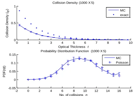
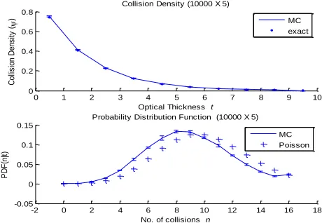
, the probability of having a collision in a region is small and the CE is bound to give an inaccurate result. This is illustrated in the figures below for a sample size of 1000X5. The discrepancy remains even as the sample size is increased to 100000X5. However, the results improve as the size of the regions is increase from 0.5 to 1.0 optical units. For the CE to provide reliable results in an MC simulation, the size of the region, or mesh in a deterministic analogy, must be larger than an optical unit. In case the mesh size can not be increased, the track-length estimator (TLE) should be used instead of the CE.0 1 2 3 4 5 6 7 8 9 10
0 0.5 1
Collision Density (1000 X 5)
Optical Thickness t
C
o
lli
s
io
n
D
e
n
s
it
y
(
)
MC exact
-2 0 2 4 6 8 10 12 14 16 18
-0.05 0 0.05 0.1 0.15
Probability Distribution Function (1000 X 5)
No. of collisions n
P
D
F
(n
|t
)
MC Poisson
0 1 2 3 4 5 6 7 8 9 10 0
0.2 0.4 0.6 0.8
Collision Density (10000 X 5)
Optical Thickness t
C
o
lli
si
o
n
D
e
n
si
ty
(
) MC
exact
-2 0 2 4 6 8 10 12 14 16 18
-0.05 0 0.05 0.1 0.15
Probability Distribution Function (10000 X 5)
No. of collisions n
P
D
F
(n
|t)
MC Poisson
Fig. 2. Monte Carlo simulation, 10000 particles and 5 batches, for a 1-D slab of thickness 10 optical units, with forward scattering and 10
regions.
As discussed above, the estimator for a first derivative for
is obtained as
(
1
)
(
)
(
p
)
p
n
t
t
n
p
n
where the estimate is obtained in a single ‗run‘.
VI. CONCLUSION
We have carried out a comparison of two deterministic methods with Monte Carlo analog simulation for computing the radiative flux for flat isothermal plates and have shown the effort required in each method. W hile MC is computation-intensive, it has the advantage of being applied to complex geometrical configurations and is capable of handling realistic scattering laws for thermal radiation. This is a great advantage over deterministic methods. We have also considered the MC random-walk in some detail to show the approach by which derivative quantities can be sampled during a full simulation. This work is useful as a didactic exercise to extend MC to complex problems for engineering design sensitivity.
REFERENCES
[1] J. P. Holman, Heat Transfer, Seventh Edition, McGraw-Hill Inc., 1992.
[2] M. Quinn Brewster, Therm al Radiative Transfer and Properties, John Wiley & Sons, Inc., 1992.
[3] Michael F. Modest, Radiative Heat Transfer, Second Edition, Academic Press, 2003.
[4] Gökmen Demirkaya, Monte Carlo Solution of a Radiative Heat T ransfer Problem in a 3-D Rectangular Enclosure Containing Absorbing, Emitting, and Anisotropically scattering medium, M.S. T hesis, Department of Mechanical Engineering, Middle East T echnical University, December 2003.
[5] J. Spanier and E. M. Gelbard, Monte Carlo Principles and Neutron Transport Problem s, Addison-Wesley Publishing Company, 1969. [6] E. A. Straker, P. N. Stevens, D. C. Irving and V. R. Cain, T he
MORSE Code – A Multigroup Neutron and Gamma-ray Monte Carlo T ransport Code, Oak Ridge National Laboratory, ORNL -4585 (1970)
[7] J. F. Briesmeister, Ed., ―MCNP —A General Monte Carlo Code for Neutron and Photon T ransport‖, LA-7396-M, Los Alamos National Laboratory (1986).
[8] M. Ragheb, Slowing Down in Hydrogen or Particle T ransmission through a Slab Shield, University of Illinois, Urbana-Champaign, 2003.
[9] H. Rief, ―Generalized Monte Carlo Perturbation Algorithms for Correlated Sampling and a Second-Order T aylor Series Approach‖, Annals of Nuclear Energy, vol. 11, 9, 455 (1984).
[10]Z. U. Koreshi and J. D. Lewins, "T wo -group Monte Carlo Perturbation T heory and Applications in Fixed-Source Problems",
Progress in Nuclear Energy, vol. 24, pp.27-38 1990.