149 Abstract— Localization is a problem which has been studied for many years and it is an unavoidable problem when dealing with the sensor nodes. Typically, in localization a target to be localized moves at random within the coverage of the sensor network. Current localization systems are using simplistic movement models and they do not consider energy consumption of sensor nodes. The problem considered in this paper is exploration of an unknown environment with the goal of finding the nodes at an unknown location(s) using location aware (LA) nodes. In this paper, a Particle Swarm Optimization (PSO) based energy efficient localization method is proposed. The localization is performed by learning movement patterns and their parameters such as Received Signal Strength (RSS) and angle of arrival (AoA) to guide LA nodes for locating target(s). Only a small number of sensors are activated to track and localize the target; while others are turned into sleep mode thus minimizing the energy consumption. The proposed method is evaluated on various mobility models and by the simulation results it is shown that our proposed method increases the accuracy of localization by minimizing estimation errors with reduced energy consumption and overhead.
Index Terms— angle of arrival (AoA), Localization, Mobile Wireless Sensor Networks, Particle Swarm Optimization, Received Signal Strength (RSS).
I. INTRODUCTION
Sensor networks are considered as dense wireless networks of small and low-cost sensors which collect and distribute the environmental data. Monitoring and controlling of physical environments are assisted by the wireless sensor networks even from the remote locations with better accuracy. Environmental monitoring, military purposes and gathering sensing information in hospitable locations are the applications of the wireless sensor networks. Due to their inexpensive nature and adhoc method of deployment, sensor networks have several energy and computational constraints. By utilizing more energy efficient routing, localization algorithms and system design, considerable research has been focused to overwhelm these deficiencies [1].
There are two canonical applications in wireless sensor networks and these applications are closely related to each
Mr. J.Jasper Gnana Chandran, Assistant Professor & Head, Department of EEE, Francis Xavier Engineering College, Tirunelveli, Tamilnadu, India (ph: +91 9443201279, e-mail: [email protected])
Dr. S. P. Victor, HOD of Computer Science & Director of Computer Science Research Centre, St. Xavier’s college (Autonomous), Palayamkottai, Tirunelveli, Tamilnadu. India (e-mail: [email protected])
other. They are
• Localization and • Tracking
Generally, sensor nodes are arranged in an ad-hoc manner in all the cases and the nodes have to arrange themselves in some spatial co-ordinate system. The nodes in the sensor networks are unaware of their location because they are arranged in an unplanned manner. Estimating the position or spatial coordinates of wireless sensor nodes is the problem defined in the localization and it is considered as a critical issue for WSNs. Routing protocols can operate more efficiently by exploiting the location information.
Global Positioning system (GPS) is one of the solutions for this problem. But by using GPS, it experiences some demerits such as:
• GPS can work only in outdoors.
• GPS receivers are expensive hence they are not appropriate in the construction of small cheap sensor nodes.
• In the presence of any obstacle like dense foliage etc, GPS cannot work.
Hence the sensor nodes have to organize themselves and establish their positions into a coordinate system without depending on an existing infrastructure [1]. Localization is a problem which has been studied for many years and it is an unavoidable problem when dealing with the sensor nodes [2]. Depending upon the quality of localization, tracking attains fine-grained or coarse-grained location of the specific target [3].
A. Problem Identification and Solution
Usually in a tracking scenario a target to be localized moves at random within the coverage of the sensor network. In order to predict the moving trajectory, existing work used the prior probability and probability distribution function (PDF). But there is no guarantee that the prior positions would influence the future status of the target.
But the energy consumption of the sensor nodes is not considered by any of these proposed localization systems. When the energy of sensor networks decreases then the performance also gets degraded. Due to the limited on-board resources of sensor nodes, energy saving is considered as the fundamental for the system design in wireless sensor networks. In order to extend the lifetime of sensor networks, an extensive amount of solutions have been developed to conserve energy.
In order to improve the existing localization techniques, Particle swarm optimization (PSO) based energy efficient localization technique (EELT) is proposed in this paper. Based on various mobility models, the proposed method is evaluated. The localization is performed by learning
Optimized Energy Efficient Localization
Technique in Mobile Sensor Networks
150 movement patterns and their parameters such as velocity and acceleration. Based on a combined measurement including information utility, communication cost, and residual energy, the energy conservation and the subset of sensor nodes are activated. Only a small number of sensors are activated to track and localize the target; while others are turned into sleep mode, in order to reduce the energy consumption. In order to analyze the set of localization algorithms and to optimize the proposed localization algorithm, the Particle Swarm Optimization (PSO) technique is utilized.
A population based stochastic optimization technique which shares many similarities with evolutionary computation techniques such as Genetic Algorithms (GA) is called as Particle Swarm Optimization [6]. By updating the generations, the system is initialized with a population of random solutions and recursively searches for maximum. PSO has been successfully applied in many research and application areas for the past several years. When compared with other methods, the PSO attains better results in faster and in cheaper way.
II. RELATED WORK
Zhong Zhou et al. [4] have presented a scheme, called Scalable Localization scheme with Mobility Prediction (SLMP), for underwater sensor networks. In SLMP, localization was performed in a hierarchical way, and the whole localization process was divided into two parts: anchor node localization and ordinary node localization. In SLMP, anchor nodes conducted linear prediction by taking advantages of the inherent temporal correlation of underwater object mobility pattern.
Rui Huang et al. [4] have presented a localization algorithm that allows non-GPS nodes to be localized based on heterogeneous measurements including ranging, angle and connectivity. They studied the behavior of RSSI and AoA sensory data in the context of the ad hoc localization problem using both geometric analysis and computer simulations. Their proposed algorithm followed the particle filter framework that solved the localization problem in both stationary and mobile ad hoc networks.
Minghui Li and Yilong Lu [8] has presented an algorithm which bears evaluation in unknown noise fields and harsh WSN scenarios. A maximum likelihood (ML) criterion is established by modeling the noise covariance as a linear combination of known weighting matrices. For optimization of the ML cost function, a particle swarm optimization (PSO) paradigm is presented.
Chuang-wen You, Yi-Chao Chen, Ji-Rung Chiang, Polly Huang, Hao-hua Chu [9] have proposed an energy-aware localization that adapts the sampling rate to target's mobility level, without giving up significant accuracy, in order to reduce power consumption. Based on signal strength fingerprinting an energy-aware adaptive localization system is designed, implemented, and evaluated. In order to satisfy an application's requirements on positional accuracy their system tries to adapt its sampling rate to reduce its energy consumption.
Hui Kang and Xiaolin Li, Patrick J. Moran [10] have proposed a novel measure method of information utility for
tracking and localization in wireless sensor networks (WSNs). Using a transition matrix, when the target moves arbitrarily in WSNs, it is modeled by Markov chains. The next state of the target can be obtained and the informative sensors are identified from this utility measurement.
Zhong Zhou, Jun-Hong Cui and Amvrossios Bagtzoglou [11] have proposed a scheme, for underwater sensor networks, called Scalable Localization scheme with Mobility Prediction (SLMP). In SLMP, localization is performed in a hierarchical way. The whole process of localization is divided into two parts: anchor node localization and ordinary node localization. During the localization process, by knowing the past location information every node guesses its future mobility pattern. Based on its mobility pattern which is predicted future location can be estimated.
Luca Marchetti, Giorgio Grisetti, Luca Iocchi [12] have provided a systematic analysis of Particle Filter Localization methods, which consider the different observation models to be used in the RoboCup soccer environments. Two different particle are investigated for filtering strategies and its usage. They are the well known Sample Importance Resampling (SIR) filter, and the Auxiliary Variable Particle filter (APF).
III. PSOBASED LOCALIZATION
A. System Design
The ad hoc localization problem (AHLP) has the task of finding the physical location of all nodes. Only the subset of nodes named as location-aware (LA) nodes, know their exact location. Given a network graph G=(V,E) where
}
{Vgps is a subset of the nodes in {V}i.e. {Vgps}⊂{V} are LA nodes. The locations of non-LA nodes can be found by{V}−{Vgps}.
The AHLP is non-trivial for a number of reasons: To find the location,
1. A node should know the locations of at least three LA nodes and Distance between the node and any of these LA nodes.
2. It should measure the distance and an (absolute) angle between any one LA node and a normal node
Though the measurements are correct, it is not possible for the LA nodes to surround each regular node. This is because
• MANETs may be randomly arranged
• Only a small percentage of nodes are LA nodes. Therefore the better solution for this, is given by estimating the nodes locations based on other nodes location (multi-hop information)
Availability of Measurements:
• Some sensory devices are needed to provide such readings.
• The algorithm requires distance or angle measurements.
151 • These algorithms need to work in a heterogeneous
environment with different location sensory capacities.
First, let us consider the scenario where the sensor readings do not include the measurement noise interference. Minimum three RSSI readings from different LA nodes and only two AoA readings are necessary to locate a node. In order to locate the node when both measurement types are available, one RSSI reading and one AoA reading from the same LA nodes are required. In such cases, for locating more nodes than the RSSI readings, better coverage must be provided by the AoA readings.
B. Localization Algorithm
In PSO the individuals are termed as particles. These particles spread in the multi dimensional search space representing a possible solution to the multidimensional problem. Each particle has fitness values for optimization and which can be evaluated by the fitness function. These particles have velocities to direct their movement. Initially PSO contains a group of random solutions and by means of updating generations it searches for optimal solution.
In iteration, updating of each particle is done by following two "best" factors.
Pb: It is the best fitness the particle has achieved so far and stored in memory.
Gb: It is the "global best" value obtained so far by any particle in the population
Lb: It is the "best" value obtained so far by any particle in the population in its topological neighbors.
After every iteration, if more optimal solution is found by the particle and population then the pbest and gbest (or lbest) are updated respectively.
The fitness function Ff, is based on the signal strength (RSSI) and angle of arrival (AoA) of the LA node. For a node
n
, the fitness function can be calculated by
) ( / )
(n RSSI n A
A
Ff = o (1)
The position of the particle is based on its previous position Ln and its velocity Vnover a unit of time:
1
1 +
+
=
n+
nn
L
v
L
(2)The velocity of a particle is computed as follows:
) (
* * ) (
*
* 1 2 2
1
1 i n n n n n
n I v k Un pb L k Un lb L
v + = + − + −
(3)
Where parameters used are: i
I = inertia coefficient n
v = current particle velocity
1
Un = uniformly distributed random number [0:1]
2
Un = uniformly distributed random number [0:1]
2 1,k
k = acceleration constants The pseudo code is as follows:
1. Get AoA and RSSI values for LA node.
2. Initialize population with random positions and velocities
3. Non LA nodes associate with another node based on the maximum signal strength received from each LA node, thus forming mini swarms
4. Evaluate fitness of each particle in swarm as per (2). 5. For each particle in each mini swarm
5.1 Find particle best (pb) – compute fitness of particle.
5.2 Ifcpb< pb, then (where cpb is currentpb) 5.2.1 Pb=cpb
5.2.2Pblocation=cloc, where cloc is the current location
5.3 End if
5.4. Find local best (lb) for the mini swarm 5.5 Lb location = location of min (all pb in this mini swarm)
5.6 Update velocity of particle as per (3) 5.7. Update position of particle as per (2) 6. End For
7. Repeat steps 5.1 through 5.7 until termination condition is reached.
IV. PERFORMANCE EVALUATION
A. Simulation Parameters
The PSO based Energy Efficient Localization Algorithm is evaluated through NS2 simulation [16]. We use a bounded region of 1000 x 1000 sqm, in which nodes are placed using a uniform distribution. The power levels of the nodes are assigned such that the transmission range and the sensing range of the nodes are all 250 meters. In the simulation, the channel capacity of mobile hosts is set to the same value: 2 Mbps. The distributed coordination function (DCF) of IEEE 802.11are used for wireless LANs as the MAC layer protocol. The simulated traffic is Constant Bit Rate (CBR).
The following table (Table I) summarizes the simulation parameters used
TABLE:ISIMULATION SETTINGS No. of Nodes 25,50,75 and 100
Area Size 1000 X 1000
Mac 802.11
Simulation Time 50 sec
Traffic Source CBR
Packet Size 512
Transmit Power 0.360 w Receiving Power 0.395 w
Idle Power 0.335 w
Initial Energy 5.1 J
Transmission Range 250,300,350 and 400 Routing Protocol AODV
Speed 5,10,15,20 and 25
B. Performance Metrics
The performance of our proposed EELT method is compared with the Bayes particle filter method [15]. We evaluate mainly the performance according to the following metrics:
152 Control overhead: The control overhead is defined as the total number of control packets exchanged.
Average end-to-end delay: The end-to-end-delay is averaged over all surviving data packets from the sources to the destinations.
Estimation Error: It is the estimation error, which indicates how close the estimated location is to the actual location
We have conducted a number of simulation experiments to validate the effectiveness of our solution by using the following mobility models
• Random Walk Model • Random Waypoint Model
• Semi-Markov Smooth (SMS) mobility Model The results are presented in the next section.
C. Results
1) Random-Walk Model
Random Walk mobility model (Brownian motion) is the simplest mobility model. In different disciplines i.e. from physics to meteorology this model is used to represent purely random movements of the entities of a system. Random Walk mobility model consists of two categories
• Random Walk with
• Random Walk with Wrapping
Random Walk with Wrapping: This model is viewed as a random waypoint. It has similarity with the Random Direction. It is used primarily because of its simplicity: unlike for the random waypoint, the distribution of location and speed at a random instant is the same.
Random Walk with Reflection: This is similar to Random Walk with Reflection, but instead of using wrapping this makes use of billiard-like reflections [14].
A. Based On Nodes
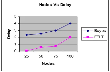
In order to test the scalability, the number of nodes is varied as 25, 50, 75 and 100.
Nodes Vs Delay
0 1 2 3 4 5
25 50 75 100
Nodes
De
la
y Bayes
EELT
Fig.1 Nodes Vs Delay
Nodes Vs Energy
0 0.5 1 1.5 2 2.5 3 3.5
25 50 75 100
Nodes
En
er
g
y Bayes
EELT
Fig.2 Nodes Vs Energy
Nodes Vs Error
0 0.05 0.1 0.15 0.2
25 50 75 100
Nodes
Er
ro
r Bayes
EELT
Fig.3 Nodes Vs Error
Nodes Vs Overhead
0 1000 2000 3000 4000
25 50 75 100
Nodes
O
ve
rh
ead Bayes
EELT
Fig.4 Nodes Vs Overhead
From Fig 1, It is seen that when the nodes are increased the delay increases. It shows the end-to-end delay occurred for both Bayes and EELT. As we can see from the figure, the delay is less for EELT, when compared to Bayes.
From Fig 2, it is seen that when the nodes are increased the energy consumption slightly increases. The figure shows the energy consumption for both the cases. As it is seen from the figure, the energy consumption is less for EELT, when compared to Bayes.
Fig 3 shows the error occurred for both Bayes and EELT. As it is seen from the figure, the error is less for EELT, when compared to Bayes.
Fig 4 shows the overhead for both Bayes and EELT. As it is observer from the figure, the overhead is less for EELT, when compared to Bayes.
B. Based On Transmission Range
153
Range Vs Delay
0 1 2 3 4 5 6
250 300 350 400 450
Range
De
la
y Bayes
EELT
Fig.5 Range Vs Delay
Range Vs Energy
0 1 2 3 4 5
250 300 350 400 450
Range
En
er
g
y Bayes
EELT
Fig.6 Range Vs Energy
Range Vs Error
0 0.05 0.1 0.15 0.2 0.25
250 300 350 400 450
Range
Erro
r Bayes
EELT
Fig.7 Range Vs Error
Range Vs Overhead
0 1000 2000 3000 4000 5000
250 300 350 400 450
Range
O
ver
h
ead Bayes
EELT
Fig.8 Range Vs Overhead
When the transmission range is varied from Fig 5, it is seen that when the transmission range is increased the delay slightly decreases it shows the end-to-end delay occurred for both Bayes and EELT. As it is seen from the figure, the
delay is less for EELT, when compared to Bayes. From Fig 6, it is seen that when the transmission range increased the energy consumption slightly increases. It shows the energy consumption for both the cases. From the figure it is observed that the energy consumption is less for EELT, when compared to Bayes. Fig 7 shows the error occurred for both Bayes and EELT. It is seen from the figure, the error is less for EELT, when compared to Bayes. Fig 8 gives the overhead for both Bayes and EELT. The overhead increases as the transmission range is increased. It is seen from the figure, the overhead is less for EELT, when compared to Bayes.
2) Random-Waypoint Model
The Random Way-Point mobility model is an example of random mobility model [13]. This model is considered as an extension of the Random Walk mobility model, because of the additional pauses between changes in direction or speed. It is an elementary model which describes the movement pattern of independent nodes by simple terms.
In the RWP model, each node moves along a zigzag line from one waypoint to the next. The waypoints are uniformly distributed over the given convex area, e.g. unit disk. At the start of each leg a random velocity is drawn from the velocity distribution. Optionally, the nodes may have so-called "thinking times" when they reach each waypoint before continuing on the next leg, where durations are independent and identically distributed random variables.
A. Based On Nodes
Nodes Vs Delay
0 2 4 6 8 10
25 50 75 100
Nodes
De
la
y Bayes
EELT
Fig.9 Nodes Vs Delay
Nodes Vs Energy
0 1 2 3 4
25 50 75 100
Nodes
En
er
g
y Bayes
EELT
154
Nodes Vs Error
0 0.05 0.1 0.15 0.2
25 50 75 100
Nodes
Er
ro
r Bayes
EELT
Fig.11 Nodes Vs Error
Nodes Vs Overhead
0 1000 2000 3000 4000 5000 6000
25 50 75 100
Nodes
Ov
er
h
ea
d
Bayes EELT
Fig.12 Nodes Vs Overhead
When the nodes are increased, Fig 9 shows the end-to-end delay occurred for both Bayes and EELT. It is seen from the figure, the delay is less for EELT, when compared to Bayes. Fig 10 shows the energy consumption for both the cases. It is seen from the figure, the energy consumption is less for EELT, when compared to Bayes. Fig 11 shows the error occurred for both Bayes and EELT. It is seen from the figure, the error is less for EELT, when compared to Bayes. Fig 12 shows the overhead for both Bayes and EELT. It is seen from the figure, the overhead is less for EELT, when compared to Bayes.
B. Based On Transmission Range
Range Vs Delay
0 0.2 0.4 0.6 0.8 1
250 300 350 400 450
Range
De
la
y Bayes
EELT
Fig.13 Range Vs Delay
Range Vs Energy
2.7 2.75 2.8 2.85 2.9 2.95
250 300 350 400 450
Range
En
er
g
y Bayes
EELT
Fig.14 Range Vs Energy
Range Vs Error
0 0.05 0.1 0.15 0.2 0.25
250 300 350 400 450
Range
Er
ro
r Bayes
EELT
Fig.15 Range Vs Error
Range Vs Overhead
0 500 1000 1500 2000 2500 3000
250 300 350 400 450
Range
O
ver
h
ead Bayes
EELT
Fig.16 Range Vs Overhead
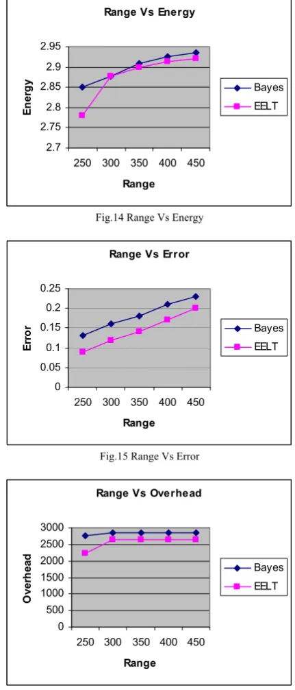
When the transmission range is varied Fig 13 shows the end-to-end delay occurred for both Bayes and EELT. It is seen from the figure, the delay is less for EELT, when compared to Bayes. Fig 14 shows the energy consumption for both the cases. It is seen from the figure, the energy consumption is less for EELT, when compared to Bayes. Fig 15 shows the error occurred for both Bayes and EELT. It is seen from the figure, the error is less for EELT, when compared to Bayes. Fig 16 shows the overhead for both Bayes and EELT. It is seen from the figure, the overhead is less for EELT, when compared to Bayes.
3) Semi-Markov Smooth (SMS) mobility model
155 can be easily and flexibly controlled to support various network scenarios. Therefore, the SMS model is a promising benchmark mobility model for both simulation and analytical study of wireless mobile networks [19].
A. Based On Nodes
Nodes Vs Delay
0 10 20 30 40
25 50 75 100
Nodes
De
la
y Bayes
EELT
Fig.17 Node Vs Delay
Nodes Vs Energy
0 0.5 1 1.5 2 2.5 3 3.5
25 50 75 100
Nodes
En
er
g
y Bayes
EELT
Fig.18 Node Vs Energy
Nodes Vs Error
0 0.05 0.1 0.15 0.2 0.25
25 50 75 100
Nodes
E
rro
r Bayes
EELT
Fig.19 Node Vs Error
Nodes Vs Overhead
0 2000 4000 6000 8000
25 50 75 100
Nodes
O
ver
h
ead Bayes
EELT
Fig.20 Node Vs Overhead
When the nodes are increased, Fig 17 shows the end-to-end delay occurred for both Bayes and EELT. It is seen from the figure, the delay is less for EELT, when compared to Bayes. Fig 18 shows the energy consumption for both the cases. It is seen from the figure, the energy consumption is less for EELT, when compared to Bayes. Fig 19 shows the error occurred for both Bayes and EELT. It is seen from the figure, the error is less for EELT, when compared to Bayes. Fig 20 shows the overhead for both Bayes and EELT. It is seen from the figure, the overhead is less for EELT, when compared to Bayes.
B. Based On Transmission Range
Range Vs Delay
0 2 4 6 8 10 12 14
250 300 350 400 450
Range
De
la
y Bayes
EELT
Fig.21 Range Vs Delay
Range Vs Energy
2.7 2.8 2.9 3 3.1 3.2
250 300 350 400 450
Range
En
er
g
y Bayes
EELT
156
Range Vs Error
0 0.05 0.1 0.15 0.2 0.25 0.3
250 300 350 400 450
Range
Er
ro
r Bayes
EELT
Fig.23 Range Vs Error
Range Vs Overhead
0 1000 2000 3000 4000 5000 6000
250 300 350 400 450
Range
O
ve
rh
ead Bayes
EELT
Fig.24 Range Vs Overhead
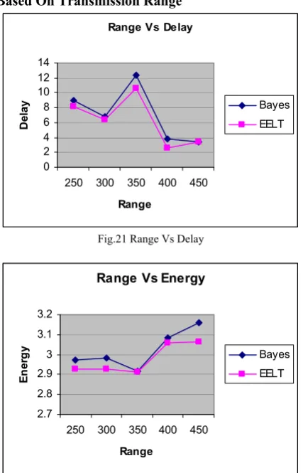
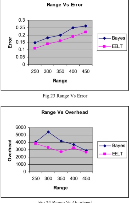
When the transmission range is varied Fig 21 shows the end-to-end delay occurred for both Bayes and EELT. It is seen from the figure, the delay is less for EELT, when compared to Bayes. Fig 22 shows the energy consumption for both the cases. It is seen from the figure, the energy consumption is less for EELT, when compared to Bayes. Fig 23 shows the error occurred for both Bayes and EELT. It is seen from the figure, the error is less for EELT, when compared to Bayes. Fig 24 shows the overhead for both Bayes and EELT. It is seen from the figure, the overhead is less for EELT, when compared to Bayes.
V. CONCLUSION
In this paper, we have proposed a Particle Swarm Optimization (PSO) based energy efficient localization technique (EELT) for wireless sensor networks. The problem considered in this paper is exploration of an unknown environment with the goal of finding the nodes at an unknown location(s) using location aware (LA) nodes. This work has demonstrated the use of a distributed PSO algorithm in which the fitness function is based on the signal strength (RSSI) and angle of arrival (AoA) of the LA node for locating target(s) in high risk environments. Essentially to reduce the energy consumption, only a small number of sensors are activated to track and localize the target; while others are turned into sleep mode. The proposed method is evaluated on various mobility models and localization is performed by learning movement patterns and their parameters. By the simulation results we have shown that our proposed method increases the accuracy of localization by minimizing estimation errors
with reduced energy consumption and overhead.
REFERENCES
[1] A.Bharathidasan and V.A.S. Ponduru. Sensor networks: An overview,
available online: http:// wwwcsif.cs.ucdavis.edu/bharathi/sensor/survey.pdf.
[2] V. Ramadurai, M. L. Sichitiu, 2003. “Localization in wireless sensor networks: a probabilistic approach”.2003, International conference
on Wireless Networks (ICWN03), pages 275-281.
[3] Hui Kang, Xiaolin Li, Patrick J. Moran, 2007. "Power-Aware Markov Chain Based Tracking Approach for Wireless Sensor Networks", Wireless Communications and Networking Conference.
[4] Z. Zhou, J.H. Cui, A. Bagtzoglou, 2008. "Scalable localization with mobility prediction for underwater sensor networks", In
INFOCOM'08.
[5] P. Bergamo, G. Mazzini, 2002. “Localization in Sensor Networks with Fading and Mobility”, In IEEE PIMRC.
[6] R Huang, ZAruba, 2007. "Incorporating Data from Multiple Sensors for Localizing Nodes in Mobile Ad Hoc Networks", IEEE transactions on mobile computing.
[7] http://www.swarmintelligence.org/
[8] Wu Xiaoling, Shu Lei, Wang Jin, Jinsung Cho1, and Sungyoung Lee, 2005. ” Energy-efficient Deployment of Mobile Sensor Networks by PSO”, Springer Berlin / Heidelberg.
[9] Chuang-wen You, Yi-Chao Chen, Ji-Rung Chiang, Polly Huang, Hao-hua Chu, 2007. ” Sensor-Enhanced Mobility Prediction for Energy-Efficient Localization”, IEEE.
[10] Hui Kang and Xiaolin Li, Patrick J. Moran,” Power-Aware Markov Chain Based Tracking Approach for Wireless Sensor Networks” Wireless Communications and Networking Conference 2007 IEEE. [11] Zhong Zhou, Jun-Hong Cui and Amvrossios Bagtzoglou, 2008. ”
Scalable Localization with Mobility Prediction for Underwater Sensor Networks”, IEEE, 2008.
[12] Luca Marchetti, Giorgio Grisetti, Luca Iocchi, 2007.” A Comparative Analysis of Particle Filter based Localization Methods”, Springer Berlin / Heidelberg.
[13] Mobility Model @ NetWis Lab.htm
[14] Jean-Yves Le Boudec and Milan Vojnovi,” Perfect Simulation and Stationarity of a Class of Mobility Models” TECHNICAL REPORT IC/2004
[15] Wojciech Zajdel, Ben J.A. Krose, Nikos Vlassis,” Bayesian Methods for Tracking and Localization”, 2005, Self Evaluation of the Informatics Institute University of Amsterdam.
[16] Network Simulator: www.isi.edu/nsnam/ns
Mr. J.Jasper Gnana Chandran received his B.E from M.S University, M.E from Anna University Chennai, Tamilnadu, India. Currently he is working as Asst. Prof & Head in EEE dept in Francis Xavier Engineering College, Tirunelveli, Tamilnadu. He is pursuing his Ph.D degree in Bharathiyar University, Tamilnadu, South India in the area of Sensor Networking. He has published several papers in national conferences and also he has written a book in Electrical Engineering. His area of interest includes Control System, Sensor network and Wireless Networking. He is a member in ISTE. He has organized Several Conferences and Seminars at national and state level.