Analysis of GPS Single Point Positioning and
Software Development
1
Pragyan Paramita Das,
2Dr. Shinichi Nakamura
1,2Dept. of Remote Sensing and GIS, Asian Institite of Technology, Thailand
Abstract
When it comes to GPS positioning we all have an overview of how it works. Various soft wares commercial or free are also provided to perform positioning with accurate results, for example RTKLIB. Have we ever wondered how the parameters like elevation mask angle and ionospheric error on and off conditions are affecting the GPS positioning. Text books generally emphasize to the basic theory of understanding the process but not how these parameters are affecting the positioning results. This paper aims to make the first attempt to show the clear picture of the performance enhance of GPS Positioning on proper knowledge of input parameters. A case of static positioning of a receiver has been shown in this paper. A simple effort has been done to make users aware of RINEX observation and Navigation file structure. The algorithm and code was developed and tested under MATLAB environment. The statistical results are quite interesting and plotted effectively to show the dramatic influence of parameters affecting positioning result. This paper aims to make users understand the behavior of Positioning in best simple way and to bring out the ideal condition to achieve the effective results for GPS Positioning.
Keywords
GPS Point Positioning, Ionospheric Error, Elevation Mask, MATLAB, RINEX, Tropospheric Error
I. Introduction
GPS is a Global Positioning System based on satellite technology. The basic principle of GPS is to calculate the range between the receiver and a few simultaneously supervise satellites. The positions of the satellites are predicted and transmitted along with the GPS signal to the user. The known position of the satellites and the measured distances between the receiver and satellite gives the receiver location. The whereabouts change of receiver, is then the velocity of the receiver. The main use of the GPS are positioning and navigating [1]. As we look back we see the background of GPS that says it was first designed and contrived by the U.S. Department of Defense [2, 10]. In 1978 the first GPS was launched, but it was fully operational in the mid-1990s.Twenty Four satellites together makes a GPS constellation. There are 6 orbital planes with 4 satellites in each plane. The orbital planes escalating nodes are bent on at 55 degrees. Each GPS satellite is in a nearly circular orbit with a semi major axis of 26578 km and a period of about twelve hours. Each satellite carries 4 atomic clocks.
A. GPS Positioning (C/A Code)
GPS point positioning uses only one GPS receiver .This receiver determines the user’s position instantly by determining the pseudo code ranges, while four or more satellites are visible. From the civilian C/A-code receivers it was observed that the expected horizontal GPS positioning that can be performed with relatively low accuracy [2]. In this study we are going to learn more precisely about single or point position.
1. Point Positioning System
The point positioning is a way to determine the user’s position
with the help of a single frequency receiver. In this method the user’s receiver simply measures the distance between the receiver and the satellites and then with the help of a triangulation method to find out the user’s co-ordinate. These 3-D co-ordinates require at least 3 satellites to measure its distance but in most cases 4 satellites are taken to reduce the timing error. This receiver is either operated in a static or dynamic mode [4-5]. The accuracies obtained here completely depend on the user’s quality of GPS receiver selected, area, period of the observation time and many other factors. When we use static and long term absolute GPS measurements with enhanced equipment and post processing techniques, we can achieve a high level accuracy of 1 meter. Hence after finding out the co-ordinates of the satellites we can put them in further pseudorange equation for unknown receiver position [3]. If we take into consideration more pseudo ranges it will only increase the redundancy of the solution. Suppose if we have seven satellites, we shall get 7 pseudo ranges equation yet only 4 unknown results.
2. GPS Point Positioning Accuracies:
The accuracy determination is very complicated and unstable due to various factors that contribute towards error in the GPS observation. But we can still observe horizontal positional accuracies in a Single Point Positioning in range of 10m to 30m [10]. Some of the more significant components of the error budget include: receiver and antenna quality, reference frames, satellite geometry, receiver platform, atmospheric condition, receiver noise, receiver mask angle, location computation and multipath errors.
In general, there are two main components that determine the accuracy of a GPS position solution:
Geometric Dilution of Precision (GDOP) •
User Range Error (URE) •
In surveying terms while computing trilateration position GDOP is referred to as “strength of figure”. It varies rapidly with time since the satellites are moving. The accuracy of the individual range measurement to each satellite is known to be URE. It also varies between different satellites, atmospheric conditions, and receivers. Absolute GPS are largely dependent on which code (C/A or P-Code) is used to determine positions which gives absolute range accuracies. These range accuracies (URE), when coupled with the geometrical relationships of the satellites during the position determination (GDOP), result in a 3-D confidence ellipsoid that depicts uncertainties in all three coordinates. Given the continuously changing satellite geometry, and other factors, GPS accuracy is time/location dependent. Error propagation techniques are used to define nominal accuracy statistics for a GPS user.
3. GPS Range Error Factors
35
tropospheric and ionospheric refraction , atmospheric absorption and satellite clock and electronics inaccuracies. Moreover the random observation errors and the unexplainable and unpredictable time variation in GPS can neither be eliminated nor modeled to correct. These above errors are discussed below which are more or less eliminated in GPS [6, 8].
(i). Ephemeris Errors and Orbit Perturbations
The error in prediction of satellite position is called satellite ephemeris error. When transferred to user in the satellite data, these are almost less than 8m i.e. 95% [7].Due to many factors affecting directly to the satellite orbits these errors are really hard to measure directly. Even when modelling the orbit of the satellite it becomes nearly impossible to accurately measure or compensate these errors. These produce equal error shifts and in calculated point positions and it is not practical for real time point positioning applications.
(ii). Clock Stability
The time measurements are really important for GPS readings that contain rubidium and cesium time standards that are usually accurate to 1 part in 10 12 [s/s] and 1 part in 10 13[s/s] respectively, while most receiver clocks are activated by a quartz standard accurate to 1 part in 10 8. A time offset is the difference between time recorded by satellite clock to that recorded by the receiver clock.
The time co-ordination between the GPS satellite clocks is kept to within 20 nanoseconds (ns) through the broadcast clock corrections as determined by the ground control stations and the synchronization of GPS standard time to the Universal Time Coordinated (UTC) to within 100 ns. Random time drifts are unpredictable, thereby making modelling difficult.
The time co-ordination between the GPS satellite clocks is kept to within 20 nanoseconds (ns) through the broadcast clock corrections as determined by the ground control stations and the synchronization of GPS standard time to the Universal Time Coordinated (UTC) to within 100 ns. Random time drifts are unpredictable, thereby making modelling difficult [9].
(iii). Ionospheric Delays
Ionospheric delay of a microwave signal depends on its frequency. These signals get dispersed or scattered when they pass through a highly charged environment like the ionosphere therefore creating an error in GPS range value.
It is difficult to apply Ionospheric correction in C/A phase positioning. Single-frequency receivers used in a point and differential positioning mode typically rely on ionospheric models that model the effects of the ionosphere. But here for C/A method of positioning we have used the Klobuchar Model according to IS-GPS-200 method to calculate ionospheric delay [7].
(iv). Tropospheric Delays
The troposphere does not disperse the L1 band signals but it gets refracted due to the moisture content in lower atmosphere. To calculate the troposphere delay we can use a modified model Saastamoinen Model.
(v). Multipath
This occurs when the signal arrives to the receiver at more than one path. This occur generally at large reflective surfaces like metal surfaces or buildings. This creates inaccurate GPS positions when processed. The high quality receiver like Choke Link Antenna
can help in minimizing the multipath effect. Whereas taking the mean of GPS signals over a course of time (i.e. different satellite configurations) also helps in reducing the effects of multipath [11].
VI. Receiver Noise
The ability of the GPS receiver to measure a finite time difference greatly affected by the receiver noise that creates a variety of errors. The noise can be considered predominantly arising from signal processing, clock/signal integration and correlation methods, receiver resolution, signal noise and others [11].
II. Location and Receiver Description
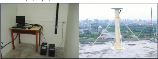
For static point positioning we considered the Chulalogkorn University GPS station, Pathumwan, Bangkok, Thailand. The station id is given as CUSV. It was installed in 2008-05-12. The approximate position of station is
X coordinate (m) : -1132913.7678 Y coordinate (m) : 6092530.5657 Z coordinate (m) : 1504633.5192 Latitude (N is +) : +134409.29 Longitude (E is +) : +1003202.07 Elevation (m,ellips.) : 76.06
Fig. 1: Chulalogkorn Station
The receiver used in Chulalogkorn station is Trimble Netrs, this monitors and surveys continuously providing good accuracy for GPS. The receiver strong point can be research of atmosphere, data generation of surveys and the infrastructure related to geodetic. When it comes to tuff environments and applications related to science, Trimble can be ideal, since it has GPS stations spread widely.
If we talk about the features of the receiver it helps for technology tracking for GPS, more easy to set up even if at far-flung areas with the use of internet. The consumption power is very less. The receiver uses Linux framework that is much more easier to make some customization which we cannot find in other systems. It is so designed to configure all receivers in network even as because the files can be stored and used quickly. It is possible to be operated according to the requirements.
It also gives security and safe access to the configuration of receiver with a low maintenance cost. The most important feature is we don’t need a local computer for it , it can be accessed from any convenient location . If there occurs some sudden shutdown it can load from the last known good configuration.
Coming to performance specification it has a high match for L1 and L2 signals , it has a very low noise tracking to L1 and L2 signals and a very high dynamic response. It is useful for low elevation tracking.
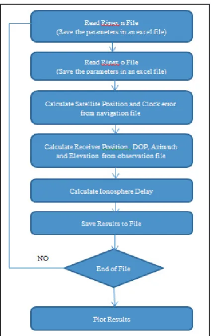
III. Methodology
The basic Methodology involves calculation of receiver position first and then apply corrections.
Fig. 2: Workflow for Point Positioning
A. Rinex n File Structure
Fig. 3: Structure of Navigation File
1st Line of Data Part
PRN 2, Year 2015, Feb, 15,1 hour 59minutes and 49 seconds then express the observer clock toc that are the clock correction coefficients
af0 = 5.480237305164D-04[s/s2], af1= 2.273736754432D-12[s/s], af2=0[s]
We can use clock correction coefficients to fix clock error as below
tt = tT-b
b=af0 +af1 (tT- t
oc)+ af2 (tT- toc)2 - TGD
where,
tT = Satellite Clock , tt = true GPS time
TGD=Group Delay parameter
2nd Line of Data Part
IODE(Issue of data , ephemeris): 5.000 Crs(correction of orbit1): -7.18750[m]
Δn(correction for mean motion): 5.069721445D-09[rad/s] M0(Men anomaly): -5.006788952400D-01[rad]
3rd Line of the Data Part
Cuc(Correction for orbit2): -2.793967723846D-07[rad] e(Eccentricity): 1.437649840955D-02
Cus(Correction for orbit 3) : 9.935349225998D-06[rad] √a(semi major axis): 5.153765422821D+03[m1/2]
4th Line of the Data
toe(Time of ephemeris): 7.184000000000D+03[s] of GPS week Cic(Correction for orbit 4): 5.587935447693D-08[rad]
Ω0(Ascending Node): -2.062240155209D-01[rad] Cis(Correction for orbit 5): 2.682209014893D-07[rad]
5th Line of Data Part
i0(inclination): 9.408638267321D-01[rad]
Crc(Correction of orbit6): 1.805937500000D+02[m] ω(Argument of perigee): -2.321076091324D+00[rad]
Ω(Change rate of ascending node): -8.461066723105D-09[rad/s]
6th line of data
i(change of rate of inclination): 3.903734034763D-10[rad/s] Code on L2 channel : 1
W/N(GPS week Number): 1.832000000000D+03[rad] L2 P data flag:0
7th Line of Data Part
URA(Ranging Accuracy): 2.000000000000D+00[m] SVhealth(health of GPS): 0.000000000000D+00 TGD(Group delay): -2.048909664154D-08[s]
IODC(Number of Issue of data, clock): 5.000000000000D+00
8th Line of Data Part
tot(Transmission time of message): 1.800000000000D+01[s] of GPS week
FIT(Fitting interval): 4.000000000000D+00[h]
There are total number of 21 parameters given for each satellite at one epoch. Count the total number of epoch and read the navigation file to save the parameters to an excel file.
B. Rinex o File structure
37
The header contains the information of GPS station and summary of the observation data type.
Fig. 5: Body of Rinex Observation File
From the first line of the observation file the 31st character tells us the number of satellites followed by the satellite number shown at that epoch.
From the second line the type of data related to each satellite is given. So for second line it shows us the L1 L2 P1 C1 S1 S2 observation for PRN 13. Similarly the third line for PRN 24 till PRN 12. This is for one epoch. We need to read the whole observation file and calculate the total number of epoch present and save the structure to an excel file. Generally the difference between each epoch is 30seconds.
C. Satellite Position Calculation
The satellite position is calculatd from the parameters in navigation file. The clock error is already corrected according to equation(1). The position of GPS satellite in ECEF co-ordinate is calculated as,
(1)
1. Receiver Position and DOP calculation
The receiver position was derived using Least Mean Square Method. In Least Mean Square Method the iteration continues till the error is reduced to zero. Four pseudorange observations are needed to resolve a GPS 3-D position. Traditionally, there are often more than four satellites in a story. We require a minimum of four satellite ranges to resolve the clock biases contained in both the satellite and the ground-based receiver. Thus, in solving for the X-Y-Z co-ordinates of a point, a fourth unknown (i.e. clock bias--Dt) must also be included in the solution. The solution of the 3-D position of a point is simply the solution of four pseudorange observation equations containing four unknowns, i.e. X, Y, Z, and Δt.
A pseudorange observation is the combination of true range and the satellite/receiver clock biases and other effects given as
(2)
Where,
R = observed pseudorange
Pt = true range to satellite (unknown) c = velocity of propagation
Δt = clock biases (receiver and satellite) d = propagation delays due to atmospheric conditions
2. Error Correction
The ionospheric error correction is applied to the receiver position. Since we used single carrier frequency C/A code for positioning, the Kobluchar model of ionosphere delay was used to correct the position. The results were saved to file.
IV. Results and Discussion
The positioning results were calculated according to the steps described above. This was affected by various parameters and these parameters were studied carefully to check the positioning accuracy. Positioning on 15/feb/2015 at Chulalongkorn University was done. Rinex observation file cusv0460.o and Rinex navigation file cusv0460.n was downloaded from igscb.jpl.nasa.gov website. The number of epoch calculated were 2879.
We assume origin of graph, Lat=13.7359[deg], Lon=100.5339[deg], h=76.06[m] which were given by RINEX.o header. The troposphere correction was already applied which varies between 0-20 meter for 5 degrees elevation mask and from 0 – 50 meters without elevation mask. In order to properly understand the effect of elevation mask parameter first non weighted analysis was done and later on checked with weighted analysis.
A. Non Weighted Analysis
In non-weighted analysis we reduce the number of satellite selection with the help of elevation mask. If we consider an elevation mask angle of 5 degrees then the satellites having elevation less than 5 degrees at that point of epoch will be eliminated and rest satellite will be used for the receiver position calculation.
Fig. 6: Non Weighted Analysis With Different Elevation Mask
Table 1: Statistical Error of Elevation Mask 0 , 10, 20 and 30 Degrees
NUM
of Data 2879
Unit=m
MASK
0 EW` NS UD 2D H 3D
AVG 2.287 -0.538 3.1856 3.838 5.1493 6.824 STD 2.172 2.181 6.0197 1.856 4.4596 4.241
RMS 3.155 2.867 6.8107 4.263 6.8107 8.035
MAX 16.47 9.171 16.271 18.92 55.181 58.33
MIN -17.4 -7.41 -55.18 0.089 0.0011 0.975
MASK
10 EW NS UD 2D H 3D
AVG 2.212 -0.586 3.7929 3.521 4.3643 5.940 STD 1.475 2.679 4.1928 1.480 3.5942 3.356
MAX 8.981 4.533 20.844 9.708 20.844 21.20
MIN -2.73 -7.328 -4.862 0.111 0.0001 1.186
MASK
20 EW NS UD 2D H 3D
AVG 1.630 -0.111 3.1599 3.209 4.4619 6.021 STD 1.756 2.615 25.747 1.515 25.553 25.48
RMS 2.396 2.618 25.94 3.549 25.944 26.18
MAX 13.15 15.95 1331.0 20.68 1331.0 1331.
MIN -8.70 -5.927 -198.8 0.081 0.0019 0.345
MASK
30 EW NS UD 2D H 3D
AVG 1.640 0.204 2.8732 3.288 5.8973 7.417 STD 2.482 2.560 30.032 2.153 29.587 29.50
RMS 2.975 2.569 30.169 3.931 30.169 30.42
MAX 45.82 15.956 1331.0 46.40 1331.0 1331.1
MIN -30.7 -11.63 -440.1 0.081 0.0001 0.4105
According to DOT we should keep an elevation mask angle of 10 – 20 degrees. Now why is it advised so. This can be studied from the above statistics results how with the increase in elevation mask the standard deviation reduced but again at 30 degrees mask the trend reversed and standard deviation increased. Same with RMS error and other parameters. So from the above statistics we can say it is advisable to keep an elevation mask angle between 5 degrees to 20 degrees for better positioning result.
For our study we considered the elevation mask angle of 5 degrees in-order to reduce the processing time and quick results. Then after the 5 degree mask angle an ionospheric on/off condition as checked with the positioning result. The ionosphere delay is a major factor playing in the GPS positioning. We know that ionosphere spreads from 500 to 1000 km so the speed of signal is mostly affected during travelling. The carrier phase is not so long but the pseudo range is , so the correction is done to pseudorange. We add the delay to pseudorange.
(a) (b)
Fig. 7: (a) Positioning with and without ionosphere correction along EW-NS non-weighted method. (b) Positioning with and without ionosphere correction along NS-UD non-weighted method
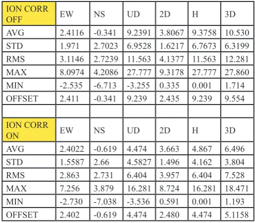
So from above figure it states that ionosphere correction helps in positioning accuracy. But with an elevation angle mask greater than 10 degrees the positioning results may increase more. But the number of satellites will decrease so in an alternate way we can use an weighted method. The statistics are shown below how the results vary with ion correction. The RMS error reduced from 3.11 to 2.86 after ionospheric correction.
Table 2: Statistics Result of Elevation Mask 5 Degrees With and Without ION Correction
ION CORR
OFF EW NS UD 2D H 3D
AVG 2.4116 -0.341 9.2391 3.8067 9.3758 10.530 STD 1.971 2.7023 6.9528 1.6217 6.7673 6.3199
RMS 3.1146 2.7239 11.563 4.1377 11.563 12.281
MAX 8.0974 4.2086 27.777 9.3178 27.777 27.860
MIN -2.535 -6.713 -3.255 0.335 0.001 1.714 OFFSET 2.411 -0.341 9.239 2.435 9.239 9.554
ION CORR
ON EW NS UD 2D H 3D
AVG 2.4022 -0.619 4.474 3.663 4.867 6.496 STD 1.5587 2.66 4.5827 1.496 4.162 3.804
RMS 2.863 2.731 6.404 3.957 6.404 7.528
MAX 7.256 3.879 16.281 8.724 16.281 18.471
MIN -2.730 -7.038 -3.536 0.591 0.001 1.193 OFFSET 2.402 -0.619 4.474 2.480 4.474 5.1158
B. Weighted Analysis
In a weighted method the number of satellites remain the same but we give less weight to the low elevation satellites and try positioning. At first with ionospheric correction on , the weight was put on and off to check accuracy.
(a) (b)
Fig. 8: (a). Positioning with and without ionosphere correction along EW-NS weighted method, (b). Positioning with and without ionosphere correction along NS-UD weighted method
From the above results we can analyze that weighted method with ionosphere correction gives us the best appropriate results. The statistics drawn from the above analysis shows that the maximum and minimum deviation as compared from the non-weighted analysis, weighted analysis showed more better results.
Table 3: Statistic Results of Applying No Weight and Weight to Positioning
NUM OF
Data 2879
Unit=m
No
Weight EW NS UD 2D H 3D
AVG 2.287 -0.53 3.195 3.838 5.152 6.827 STD 2.172 2.816 6.019 1.856 4.460 4.243
RMS 3.155 2.867 6.815 4.263 6.815 8.039
MAX 16.478 9.171 16.281 18.924 55.171 58.327
MIN -17.41 -7.41 -55.17 0.0896 0.0017 0.9841 OFFSET 2.287 -0.53 3.195 2.350 3.195 3.966
Weighted EW NS UD 2D H 3D
39
STD 1.393 2.293 3.243 1.246 2.814 2.515
RMS 2.384 2.308 4.678 3.319 4.678 5.736
MAX 7.148 3.733 14.362 7.976 14.362 15.600
MIN -2.430 -5.16 -4.665 0.241 0.001 1.129 OFFSET 1.935 -0.26 3.371 1.953 3.371 3.896 So from above table we conclude that weighted positioning gives us better result but when we consider weighted analysis with the ionospheric error it gives the best accuracy of near error of 3.3 meters.
Finally, the positioning results for Chulalogkorn University Receiver Station was,
Table 4: Positioning Result of Chulalogkorn University
Chulalogkorn
University X Y Z
AVG -1132915 6092534 1504633 STD 1.7087 3.4029 1.7944
MAX -1132911 6092545 1504636
MIN -1132922 6092526 1504628 When we calculated the Latitude Longitude and Height we got results as below,
Lat = 13.7359 deg +/-0.000 deg Long = 100.5343 deg +/- 0.000 deg Height = 73.9034 m +/- 3.6760 [m]
DOP is considered important when it comes to positioning. A good DOP provides more precision. Generally it is considered to be a distinct property to evaluate the geometric arrangement from receiver to satellite. We can say DOP is recorded to be less if the number of satellites are more. The wider the angle of satellites available at that moment gives better DOP.The DOP of Chulalogkorn station along time series of XYZ was normalized by average. Where a GDOP is considered to be ideal if below 1 meters. In this case we had varying GDOP in between 0.5 to 2 considering it to be excellent.
C. Comparison With Commercial Software RTKLIB
To check the accuracy of our MATLAB code we compared the results with commercial software RTKLIB. This is an open source software for GNSS precise positioning. It consists of program libraries that are portable and can be used easily. The results achieved were quite good .
Fig. 9: (a) EW, NS and UD Results of RTKLIB Indicated in Red and Our Script in Blue Respectively
V. Conclusion
The main aim of the study was to learn the basics of GPS positioning and to develop positioning script using MATLAB environment. This was achieved. The positioning involved C/A method of positioning. The algorithm was at first written down and understood for better understanding and then later on analyzed. Since, many students only consider analyzing results
using commercial software hence it lacks depth of understanding of individual parameter related to the process and analyze blindly. Experimenting can become easy if we understand the process by our self and then analyze things. It became easy to gain an idea of writing codes and changing values. All the important aspects related to positioning was tried to cover including the GDOP, Troposphere and Ionosphere effects and angle of elevation , the weighted and non-weighted method.
The algorithm evaluated the positioning with respect to elevation mask angle with non-weighted analysis and weighted analysis. The angle of elevation when masked to 5 degrees yielded better results. But better results appeared with weighted analysis. The procedure followed for point positioning was least mean square technique , at first when all satellites were taken into consideration the GDOP value was high near to 3meters later on when masked to 5 degrees of elevation the GDOP value came down to 2 meters. The single point positioning can give much better results on further modification to the pseudo range algorithm. At first the positioning was done without considering troposphere and ionosphere delay and no mask so the positioning range was quite dispersed about +/- 100m. With the application of all possible correction the results drastically changed to about +/- 10m accuracy.
The conclusion hence drawn from the above statistics and result is that if we go for an weighted analysis with troposphere and ionosphere correction that yields a much accurate results that a non-weighted one. The software can be developed accordingly for positioning which can have such features to analyze how parameters and process differing can affected the positioning results, this can give us a better insight and knowledge to understand GPS positioning.
We tried comparing our software results with the commercial software available in the market like TRIMBLE and RTKLIB, the variation with the commercial software were minimal. These difference in results arise due to the troposphere and ionosphere model used in the software. But a good accuracy similar to the commercial software was achieved.
To achieve accuracy up to decimeter level we can try experimenting with the data further like checking the number of cycle slips per hour. Once we can determine the number of cycle slips it may become easier for us to predict the number of slips to a satellite. Whereas , the other parameters were not studied in this experiment like effect of Selective Availability and Data acquisition length. With this investigation considering the above conditions are the highest possible methods to get the best accuracy.
References
[1] Xu, G.,"A diagonalisation algorithm and its application in ambiguity search", Positioning, 1(04), 2009.
[2] Odijk, D., Teunissen, P. J., Zhang, B.,"Single-frequency integer ambiguity resolution enabled GPS precise point positioning. Journal of surveying engineering, 138(4), pp. 193-202, 2012.
[3] Li, C., Huang, Z., Wang, S., Wang, H., Gao, S. L.,"The Application of carrier phase smoothing Pseudo-range in GPS point positioning", CSNC2012, Guanzhou, 2012. [4] Jokinen, A., Feng, S., Ochieng, W., Hide, C., Moore, T.,
Hill, C.,"Fixed ambiguity Precise Point Positioning (PPP) with FDE RAIM", In Position Location and Navigation Symposium (PLANS), 2012 IEEE/ION (pp. 643-658). IEEE, (2012, April).
solutions, 16(2), pp. 259-266, 2012.
[6] Wang, G. Q.,"Millimeter-accuracy GPS landslide monitoring using Precise Point Positioning with Single Receiver Phase Ambiguity (PPP-SRPA) resolution: a case study in Puerto Rico. Journal of Geodetic Science, 3(1), pp. 22-31, 2013. [7] Yan, M., Xiuwan, C., Yubin, X.,"Accuracy Research
on GPS Point Positioning Using IGS Data Products", In Recent Advances in Computer Science and Information Engineering (pp. 493-498). Springer Berlin Heidelberg, 2012.
[8] Angrisano, A., Gaglione, S., Gioia, C.,"Performance assessment of GPS/GLONASS single point positioning in an urban environment", Acta Geodaetica et Geophysica, 48(2), pp. 149-161, 2013.
[9] MacGougan, G., Lachapelle, G., Nayak, R., Wang, A.,"Overview of GNSS signal degradation phenomena", Paper presented at the Proceedings of International Symposium on Kinematic Systems in Geodesy, Geomatics And Navigation, 2001.
[10] Shen, X.,"Improving ambiguity convergence in carrier phase-based precise point positioning: University of Calgary", Department of Geomatics Engineering, 2002.
[11] Li, W., Teunissen, P., Zhang, B., Verhagen, S.,"Precise point positioning using GPS and Compass observations", In China Satellite Navigation Cai, C., & Gao, Y. (2013). Modeling and assessment of combined GPS/GLONASS precise point positioning. GPS solutions, 17(2), pp. 223-236, 2013.
Ms. Pragyan Paramita Das received her Bachelor’s in Electronics and Communication Engineering from Centurion Institute of Technology, Odisha, India in 2012, her Master of Engineering is in field Remote Sensing and GIS from Asian Institute of Technology in year 2015. Her research interest includes Satellite Communication, Aerospace Technology, Remote Sensing in SAR applications, Disaster and Mitigation Preparedness and GIS. She is currently working as a Research Associate for Setinel Asia Project for JAXA under Geoinformatics Centre, Thailand.