ANN Modelling and Optimization of R with corresponding MRR on HSS T42 Steel using WEDM Process

ANN Modelling and Optimization of R

_a

with

corresponding MRR on HSS T42 Steel using

WEDM Process

A.

U.K.Vates,

N.K. Singh,

R.V. Singh

A. Research Scholar Deptt of Mech Engg, ISM Dhanbad India; [email protected]

B. Associate Professor (Workshop)), Deptt of Mech Engg ISM Dhanbad India; [email protected]

C. Professor & Head, Deptt of Mech Engg, MRIU Faridabad India,[email protected]

Abstract--

Index Term-- WEDC, Ra, HSS T42, BPANN, ANOVA, RMSE1.

1. INTRODUCTION

Wire Electrical Discharge Machining is metal removal process by means of repeated spark created between the wire electrode and work piece. It is considered as unique adaptation of conventional EDM which uses an electrode to create sparks within kerfs. WEDM process utilizes a regular travelling wire anode made up of very thin copper, tungsten and brass materials of diameter ranging 0.05- 0.35 which is used to find very good edge sharpness (Ho K.H et al., 2004). The thermal erosion mechanism during WEDM, primarily, makes use of electrical energy and then turns into thermal energy through a series of discrete electrical discharges occurring between thin wire electrode and conductive material work piece immersed in a dielectric medium (Tsai, H.C et al., 2003). The thermal energy generates a channel of plasma between wire electrode and conductive and hard work material (Shobert E.I. (1983). However, conclusion from the literature has been drawn as very high temperature ranging 8000°C - 12000°C is created within the kerfs gap during machining so that material removal may takes place by not only melting but directly

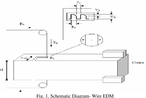
vaporization.(Boothroyd, G. Winston, A.K. 1989). Resistance and Capacitance (R-C) circuit of WEDM converts electrical energy to generate the pulsating or intermittent discharge in the form of sparks with maintaining the desire gap between the electrodes (Bawa, H.S. (2004). The electrically charged wire has the provision to perform the movement in X-Y direction to remove the work piece after each run of experiment (Qu et al 2002a, b). The concept of WEDM is illustrated in Fig.1.

Fig. 1. Schematic Diagram- Wire EDM

NOMENCLATURE

WEDM - Wire Electrical Discharge Machine WEDC- Wire Electrical Discharge Cutting ANN - Artificial Neural Network

ED – Electrode Diameter SB - Stable

TM – Machining Time T - Thickness

Ra – Surface Roughness MRR- Material Removal Rate MSE - Mean Square Error RMSE – Root Mean Square Error

A simple thermal based model to increase MRR and Ra on higher values of Ip, V or Ton (Salonitis et al. 2009). Surface features using composite material under EDM current, voltage and Ton reported as important surface roughness influencing parameters (Gatto A. et al., 1997). WEDM is used for high precision machining to all types of electrically conductive metallic alloys, tool & die, graphite and a few ceramic as well as composite materials of any hardness which cannot be machined easily by conventional machining methods and Vg, Ton, and Toff are influencing parameters of surface roughness and MRR on tool steels (Puertas I. et al,. 2003.). WEDM machining performance such as Ra, electrode wear rate and MRR with copper electrode on AISI: H3 tool steel work piece and the input parameters taken as Ip, Ton, and Toff the optimum condition for Ra was obtained at low Ip, low Ton, and high Toff and concluded that the Ip was the major factor effecting both the responses MRR and Ra (Jaharah et al., 2008). A lot of modelling techniques like ANN have already been reported for the prediction surface roughness and MRR of different conducting work materials under WEDM (Panda DK et al., 2005). (Pradhan M.K. et al 2010) also worked on same four parameters voltage, current, Ton and duty cycle for the prediction of MRR. Hybrid models of ANN and GA have been developed to predict the surface roughness of tool and die steel materials where machining time, current and voltage are inputs (Rao G. Krishna Mohana et al. 2009) RSM and ANN based prediction models have been developed which are important in evaluating the productivity and have considerable influence on the properties of the material such as wear resistant and fatigue strength (Erzurumlu O. H. et al 2007). Fractional Factorial Design of Experiment (26-2) to conduct minimum Nos. of experiments (D.C. Montgomery et al., 1991) is adopted in present investigation. 80 runs of experimental data of five different sets have been conducted and it is facilitated at three levels. WEDM process has been selected depending on the HSS T42 material characteristics and the type of responses (Ra & MRR) required to be evaluated. Two fold cross over hypothetical technique (TFCOHT) has been used to generate two distinguish models „S1‟ and „S2‟ as shown in Fig 5. where 55 runs has been used

for training under the BPANN and rest 25 runs are divided into 15 and 10 runs randomly, for validation and testing the network respectively. Four layered BPANN architecture has been used for modelling where independent process variables are Vg, Fr Ton, Toff, Wf and Wt. Best model set „S1‟ (training data) result has been tested using Analysis of Variance (ANOVA) to determine significant factors and establish the relation between factors and responses using BPANN. The optimum process parameters are much essential to achieve better surface finish with adequate material removal rate (MRR). A lot of research techniques have been reported for optimization of response, but present work uses sum of root mean square error (SRMSE) approach and achieve improvement approx more than 25% in surface smoothness under WEDM process.

2. EXPERIMENTAL SETUP

Chrome coated cylindrical pure copper wire [Resistivity ρ = 1.68x10-8 _{(ohm-m), Electrical Conductivity (σ) = 5.96x10}7

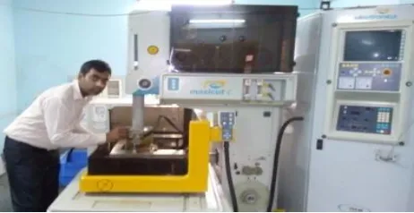
(ohm-m)-1, Temperature coefficient (K-1) = 0.003862] electrode having 0.25 mm in diameter and high tensile strength has been selected. Copper wire electrode is suitable (as far as conductivity is concerned) for performing cutting operation on 18 mm diameter of HSS T42 steel rod to cut 5 mm thickness of disk using CNC operated Wire Electrical Discharge Machine, model ELECTRONICA-MAXICUT, SLNO.-250(F: 09:0002:01) having the facilities to hold the work piece within the place provided with the help of conductive fixture so that they can complete the circuit between electrode and work piece as given in Fig.2. Very hard and conducting material (HSS T42) has been chosen in this case for its wide application in tool and dies manufacturing industries.

Table I

Chemical Composition: HSS T42 grade steel

C W Cr Mo V HRC _Conductiv

ity 1.23 % 8.92 % 3.80 % 3.10 % 2.93

% 66

±

1.6x 10 6

(S /m)

electrode. The machining performance is influenced by major independent process parameters which have been selected for experiment as characteristics of screening test. Commercials grade of deionised water [(Density= 832 kg/m3), (Electrical conductivity= 5.5 x 10-6 S/m)] has been used as dielectric fluid. 18 mm cylindrical rod of HSS T42 steel has been used as the work piece with negative polarity and the power supply has the provision to connect the 0.25 mm chromium coated pure copper tool electrode with positive polarity so that the material removal may takes place by influence of heat generated within kerfs due to applied voltage within it.

Fig. 2. HSS T42 machining using WEDM process

The surface roughness Ra of processed material have been measured precisely by using Surftest SJ-210 Surface Roughness Tester having least count of 0.001m for the travel length of 0.85 mm as given in Fig. 3.

Fig. 3. Surftest SJ-210 (Mitutoyo).

Apart from the controllable independent variable factor as Table.2, there are lot of constant parameters but they neither play the important effect of the response nor vary till the experimentation has been finished. The resolution of this fractional factorial design deals with all the significant effecting parameters on surface roughness using WEDM. Experiments were carried out randomly using suitable table so that repetitions of the runs were not done throughout.

Table III

Constant Factors during WEDM

Factors Constant Values (coded)

Jog Feed

2

Low Jog 7

Toff1 7

Sensitivity 7

2.2 Design of Experiment & Objective: Five different sets of data for Fractional Factorial Design of Experiment (26-2 = 16) have been selected at two levels so that 80 rows of experimental data can be observed at three levels of replication on HSS T42 using WEDM. Screening test on HSS T42 has been performed by authors using the D.C. Montgomery 1991approach. Factors/Levels for screening test are given in Table 2.

2.3 ANN Architecture & Training: Many more studies have been reported on the development of neural networks based on different architectures. Basically, one can characterize neural networks by its important features, such as the architecture, the learning algorithms and the activation functions. Each category of the neural networks would have its own input output characteristics and therefore, it can only be applied for modelling some specific processes. In this present work, fast Levenberg- Marquardt algorithm BPANN is employed for modelling.

In order to improve the generalisation early stop is often employed. There are two different ways in which this algorithm can be implemented: incremental mode and batch mode. In the incremental mode, the gradient is computed and the weights are updated after each input is applied to the network. In the batch mode all of the inputs are applied to the network before the weights are updated. Variations have been observed in the back propagation algorithm. The simplest implementation of back propagation learning updates the network weights and biases in the direction in which the performance function decreases most rapidly i.e. negative of the gradient. An iteration of this algorithm can be written as

Where, X_t+1 are a vector of current weights and biases, Xt is the current gradient, and gt is the learning rate.

The optimal regularization parameter can be determined by Bayesian techniques (Gencay R. et al., 2001). The hit and trial

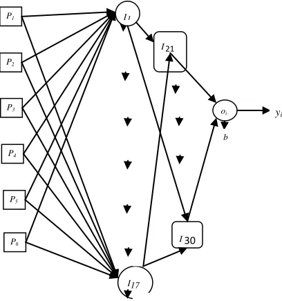
method based on literature have been adopted to find critical 7Nos. and 10 Nos. of neurons in primary and secondary hidden layers respectively which affects R- square statistic. For modelling of the best prediction Tan sigmoid activation (squashing) function is used as the infinite input to finite output range learning capability by controllable instructed programme in MATLAB 2010a. Steepest descent method used for the training algorithm to train multilayer network where values of gradient are smallest because of small changes in weights and biases. p1, p2, p3, p4, p5 and p6 are six input layer neurons and Oi is the single neurons in output layer, whereas I11-I17 and I21-I30 (7 neurons present in primary and 10 in secondary hidden layers) are hidden layers (Fig.4).

Fig. 4. Artificial Neural Network Approach

2.4 Two Fold Cross over Techniques: This is the hypothetical technique which used to split and neutralize 80 runs of experimental data set into two parts „S1‟ and „S2‟ model set. Each model also split out sequentially as serial order described in Fig.5 (Set A, B) (55 runs of training & rest 25 runs for validation and testing in arbitrarily). However, the best performing model can be selected.

Fig. 5. Set-A (S1 Model)

Fig. 5. Two Fold Crossover techniques to obtain two distinguish models.

1. DATA COLLECTION AND ANALYSIS:

The models (S1 and S2) have been developed from 80 runs of experimental data performed on HSS T42 using TFCOT. Training, validation and testing results of the best performing model (S1) are presented only to analyse and optimize influencing process parameters. The correlations statistics of both the models (S1 and S2) are given in Table.5.

It indicates 55 rows of training dataset out of total 80 rows of experimental observations on HSS T42 grade steel material using WEDM, whereas 15 rows and 10 rows of data was randomly selected for validation and testing purpose during ANN modeling. Training data is only used here to train ANN network and optimize the process parameters. It also shows the best model is „S1‟ compared to the „S2‟ for HSS T42 grade steel.

P1

P2

P3

P4

P5

P6

I17

oi y_i

b I1

1

Table IV

Summary of R2_{values of Training Validation and Testing data}

Materi

al

Model R2

Value

Equation of lines

(Correlation between

Obs. & Pred. Values

of Ra)

Average

Predicted

Ra (m)

Root Mean

Square

Error (m)

Percentage

RMSE (%)

Average

% RMSE

RMSE

Concludi

ng

remarks

HSS

T42

S1, Training 0.971 y = 0.967x + 0.047 1.5965 0.005063 0.3171 0.7353

0.7353

Accepted

(Best

model) S1,

Validation

0.962 y = 0.926x + 0.111 1.4438 0.011573 0.8015

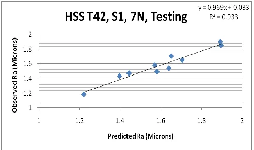
S1, Testing 0.933 y = 0.969x + 0.033 1.5834 0.01722 1.0875

S2, Training 0.974 y = 1.030x - 0.055 1.5563 0.004989 0.3205

0.7856

Not

Accepted

(more

error) S2,

Validation

0.951 y = 0.934x + 0.104 1.6086 0.01636 1.0170

S2, Testing 0.945 y = 0.935x + 0.085 1.5334 0.01563 1.0193

Correlation coefficient (R2) of the best performing model ‘S1’ (training, validation & testing data of HSS T42 grade steel):

Fig.6, Fig.7 and Fig.8 indicate the relationship between the observed and predicted correlation coefficients (R2) using 7 neurons and 10 neurons, in primary and secondary (hidden) layers respectively. Fig.6, indicates 55 rows of training data with correlation coefficient R2 = 0.991 which gives good result. The validation data having R2= 0.988 in Fig.7 and testing data having R2 = 0.979 in Fig.8, are also treated as good results.

Fig. 6. Predictions against Observations of Ra for Model- S1, HSS T42,

7N (Training dataset)

Fig. 7. Predictions against Observations of Ra for Model- S1, HSS T42,

7N (Validation dataset)

Fig. 8. Predictions against Observations of Ra for ModelS1, HSS T42, 7N

(Testing dataset)

Table V

Training Data-Best Model, S1 (HSS T42)

SN Gap Voltage

(Vg)

Flush Rate

(Fr)

Spark Time (TON)

Spark Time (TOFF)

Wire Feed (Wf)

Wire Tension

(Wt)

Surface Roughness

(Ra)

(Observed)

Surface Roughness

(Ra)

(Predicted)

Residuals Square

Material Removal (MRR) (Observed)

Volt Lit./min S S m/ min N/m2 m m (m)2 mg/min

1 30 6 1.05 160 5 300 1.5848 1.5803 2.025E-05 135

2 30 6 1.15 130 2 300 1.8174 1.8077 9.409E-05 122

3 30 6 1.15 160 2 600 2.0164 1.9835 0.0010824 118

4 60 4 1.05 130 5 300 1.5128 1.5267 0.0001932 126

5 60 4 1.05 160 5 600 1.547 1.5707 0.0005617 116

6 60 4 1.15 130 2 600 1.831 1.7461 0.007208 163

7 60 4 1.15 160 2 300 1.6798 1.6655 0.0002045 144

8 60 6 1.05 130 2 600 1.583 1.5913 6.889E-05 138

9 60 6 1.05 160 2 300 1.4224 1.4278 2.916E-05 135

10 60 6 1.15 130 5 300 1.3816 1.3622 0.0003764 128

11 60 6 1.15 160 5 600 1.5796 1.5275 0.0027144 125

12 30 4 1.15 160 5 600 1.8568 1.8489 6.241E-05 208

13 30 4 1.15 190 5 900 1.6838 1.7024 0.000346 200

14 30 4 1.25 160 8 900 1.7488 1.7412 5.776E-05 192

15 30 4 1.25 190 8 600 1.7876 1.7726 0.000225 185

16 90 4 1.15 190 8 900 1.3024 1.3006 3.24E-06 79

17 90 4 1.25 160 5 900 1.7304 1.7273 9.61E-06 127

18 90 4 1.25 190 5 600 1.4378 1.4423 2.025E-05 103

19 90 8 1.15 160 5 900 1.4256 1.4518 0.0006864 110

20 90 8 1.15 190 5 600 1.364 1.3533 0.0001145 78

21 90 8 1.25 160 8 600 1.7712 1.7798 7.396E-05 126

22 90 8 1.25 190 8 900 1.714 1.7105 1.225E-05 122

23 60 6 1.05 130 2 600 1.5433 1.5275 0.0002496 186

24 60 6 1.05 160 2 900 1.3614 1.3271 0.0011765 181

25 60 6 1.25 130 5 900 1.5708 1.5755 2.209E-05 198

26 60 6 1.25 160 5 600 1.5571 1.5495 5.776E-05 201

27 60 8 1.05 130 5 900 1.6146 1.6105 1.681E-05 218

28 60 8 1.05 160 5 600 1.5453 1.5825 0.0013838 165

29 60 8 1.25 130 2 600 1.8162 1.8289 0.0001613 276

30 60 8 1.25 160 2 900 1.6913 1.6528 0.0014823 204

31 60 6 1.25 130 5 900 2.1638 2.0306 0.0177422 170

32 60 6 1.25 160 5 600 2.053 2.1145 0.0037823 146

33 60 8 1.05 130 5 900 1.9320 1.966 0.001156 172

34 60 8 1.05 160 5 600 1.7130 1.6187 0.0088925 147

35 60 8 1.25 130 2 600 1.6813 1.6456 0.0012745 132

36 60 8 1.25 160 2 900 1.6088 1.6011 5.929E-05 128

37 90 6 1.05 130 5 600 1.2334 1.2735 0.001608 106

39 90 6 1.25 130 2 900 1.3286 1.3062 0.0005018 103

40 90 6 1.25 160 2 600 1.2813 1.3162 0.001218 96

41 30 4 1.15 190 2 900 1.7814 1.8027 0.0004537 126

42 30 4 1.25 160 8 900 1.7750 1.7471 0.0007784 219

43 30 4 1.25 190 8 300 1.7338 1.8332 0.0098804 175

44 30 6 1.15 160 8 900 1.8161 1.7912 0.00062 144

45 30 6 1.15 190 8 300 1.7842 1.7882 0.000016 150

46 30 6 1.25 160 2 300 1.8267 1.8583 0.0009986 126

47 30 6 1.25 190 2 900 1.7563 1.7502 3.721E-05 133

48 60 4 1.15 160 8 300 1.4566 1.4367 0.000396 156

49 60 4 1.15 190 8 900 1.3259 1.3106 0.0002341 154

50 60 4 1.25 160 2 900 1.3185 1.3838 0.0042641 170

51 60 4 1.25 190 2 300 1.2831 1.2226 0.0036603 159

52 60 6 1.15 160 2 900 1.4699 1.4641 3.364E-05 165

53 60 6 1.15 190 2 300 1.3536 1.3329 0.0004285 127

54 60 6 1.25 160 8 300 1.3268 1.3364 9.216E-05 158

55 60 6 1.25 190 8 900 1.3682 1.3643 1.521E-05 163

Average 1.601187 1.596570 0.005063 147

Table VI

Validation Data-Best Model, S1 (HSS T42)

SN Gap Voltage

(Vg)

Flush Rate (Fr)

Spark Time (TON)

Spark Time (TOFF)

Wire Feed (Wf)

Wire Tension

(Wt)

Surface Roughness

(Ra)

(Observed)

Surface Roughness

(Ra)

(Predicted)

Residuals Square

Material Removal (MRR) (Observed)

Volt Lit./min S S m/ min N/m2 m m (m)2 mg/min

1 30 4 1.05 130 2 300 1.852 1.8465 3.025E-05 124

2 30 4 1.05 160 2 600 1.6172 1.6278 0.0001124 116

3 30 4 1.15 130 5 600 1.715 1.638 0.005929 169

4 30 4 1.15 160 5 300 1.6418 1.6745 0.0010693 132

5 90 6 1.25 130 2 900 1.2519 1.2289 0.000529 129

6 90 6 1.25 160 8 600 1.2244 1.2694 0.002025 126

7 90 8 1.05 130 2 900 1.3217 1.3686 0.0021996 114

8 90 8 1.05 160 2 600 1.3198 1.3725 0.0027773 102

9 90 8 1.25 130 5 600 1.2758 1.2835 5.929E-05 106

10 60 6 1.05 160 2 900 1.5502 1.5885 0.0014669 134

11 90 8 1.05 130 2 900 1.1865 1.1888 5.29E-06 121

12 90 8 1.05 190 8 600 1.1768 1.1213 0.0030803 101

13 90 8 1.25 130 5 600 1.3215 1.3678 0.0021437 122

14 90 8 1.25 160 5 900 1.3105 1.3572 0.0021809 117

15 30 4 1.15 190 2 300 1.8053 1.7245 0.0065286 128

Table VII

Testing Data-Best Model, S1 (HSS T42)

SN Gap Voltage

(Vg)

Flush Rate (Fr)

Spark Time (TON)

Spark Time (TOFF)

Wire Feed (Wf)

Wire Tension

(Wt)

Surface Roughness

(Ra)

(Observed)

Surface Roughness

(Ra)

(Predicted) Residuals Square Material Removal (MRR) (Observed)

Volt Lit./min S S m/ min N/m2 m m (m)2 mg/min

1 30 6 1.05 130 5 600 1.7048 1.6544 0.00254 152

2 30 8 1.15 160 8 900 1.6502 1.7097 0.00354 232

3 30 8 1.15 190 8 600 1.5708 1.5819 0.000123 135

4 30 8 1.25 160 5 600 1.892 1.9068 0.000219 269

5 30 8 1.25 190 5 900 1.8966 1.8536 0.001849 102

6 90 4 1.15 160 8 600 1.3962 1.4381 0.001756 269

7 90 6 1.05 130 5 600 1.5812 1.4955 0.007344 106

8 90 6 1.05 160 5 900 1.4434 1.4715 0.00079 86

9 90 8 1.25 160 5 900 1.2215 1.1844 0.001376 138

10 60 6 1.05 130 2 600 1.6389 1.5382 0.01014 146

Average 1.59956 1.58341 0.029678 163.5

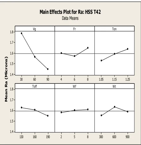
Table V represents the training data of the best depicted model and it may be used to analyse factors trained using ANOVA. Fig.9 indicates that gap voltage, flush rate, spark on time, spark off time, wire feed and wire tension have the most significant effect on surface roughness of HSS T42 under WEDM. However, it is also clear that surface roughness is inversely proportional to gap voltage and spark off time, whereas, it is directly proportional to spark on time and wire feed. Flush rate and wire tension still, seem to be imparting effects on Ra, but both opposite to each others. Only in this case of comparison, the plot of factors effect is allowed to be used. The interaction plot of Ra is also indicated in Fig.10. It indicates high flush rate at moderate wire tension leads to decrease in surface roughness. ANOVA has been used to test the null hypothesis with regard to the training data obtained through experimental processes.

90 60 30 1.8 1.7 1.6 1.5 1.4 8 6

4 1.05 1.15 1.25

190 160 130 1.8 1.7 1.6 1.5 1.4 8 5

2 300 600 900

Vg M e a n R a ( M ic r o n s ) Fr Ton

Toff Wf Wt

Main Effects Plot for Ra: HSS T42

Data Means

8 6

4 1.05 1.15 1.25 130 160 190 2 5 8 300 600 900

1.8 1.6

1.4

1.8 1.6 1.4

1.8 1.6 1.4

1.8

1.6 1.4

1.8 1.6 1.4

Vg

Fr

Ton

Toff

Wf

Wt

30 60 90 Vg

4 6 8 Fr

1.05 1.15 1.25 Ton

130 160 190 Toff

2 5 8 Wf

Interaction Plot for Ra: HSS T42

Data Means

Fig. 10. Main interaction Plot for Ra: HSS T42

It is assumed that there is no difference in treatment resources. Table.8 indicates the ANOVA for surface roughness and it indicates that Fr, Ton, Toff, Wf and Wt

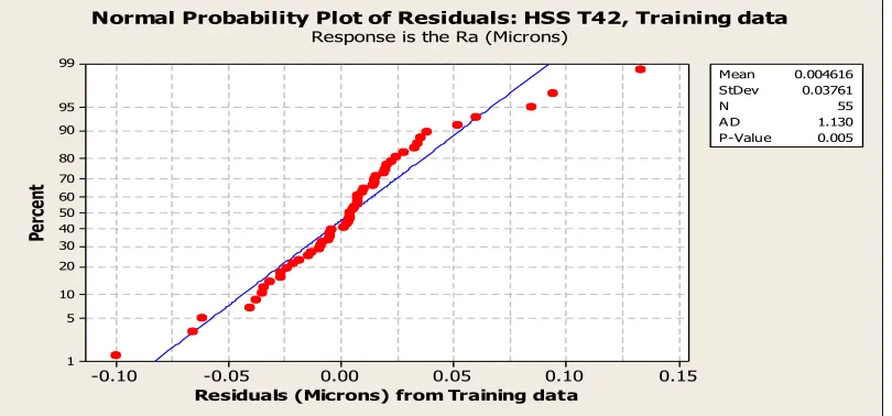
As the Nested ANOVA for Ra Table.8, indicates all the factors are most or moderate significant with Ra of HSS T42 under WEDM. are the most significant. Figures 11,12 and 13 show the normal plots of residuals. Normal distribution of error may be recast

broadly by using these methods. In all three cases normal probability plots from training, validation and testing dataset P- values obtained are less than 0.05 as indicated in Fig.11, Fig.12 and Fig.13 respectively. This indicates the model „S1‟ is verified for BPANN using ANOVA.

0.15 0.10

0.05 0.00

-0.05 -0.10

99

95 90

80 70 60 50 40 30 20

10 5

1

Residuals (Microns) from Training data

Pe

rc

en

t

Mean 0.004616

StDev 0.03761

N 55

A D 1.130

P-Value 0.005

Normal Probability Plot of Residuals: HSS T42, Training data

Response is the Ra (Microns)

Table VIII

Nested ANOVA for Ra versus Vg, Fr, Ton, Toff, Wf, Wt Source DF SS MS F-value P-value

Vg 2 0.7869 0.3934 9.06451 0.6831058

Fr 5 0.3620 0.0724 1.66820 0.1257571

Ton 11 0.4815 0.0438 1.00921 0.0760545

Toff 21 0.4127 0.0197 0.45391 0.0342069

Wf 5 0.2155 0.0431 0.99308 0.0748390

Wt 2 0.0069 0.0035 0.08064 0.0060771

Error 8 0.3472 0.0434 - -

Total 54 2.6127 - - -

0.10 0.05

0.00 -0.05

-0.10

99

95

90

80 70 60 50 40 30 20

10

5

1

Residuals (Microns)

Pe

rc

en

t

Mean -0.005827

StDev 0.04600

N 15

A D 0.797

P-Value 0.030

Normal Probability Plot of the Residuals: Validation data (HSS T42) Response Ra (Microns)

Fig. 12. Normal Probability plot of residuals from validation data

0.15 0.10

0.05 0.00

-0.05 -0.10

99

95 90

80 70 60 50 40 30 20

10 5

1

Residuals (Microns)

Pe

rc

en

t

Mean 0.01615

StDev 0.05484

N 10

A D 0.282

P-Value 0.556

Normal Probability Plot of Residuals: HSS T42 (Testing data)

Response is Ra (Microns)

Fig. 13. Normal Probability plot of residuals from Testing Data

Training and verifying the ANN model:

In order to minimize the training difficulty and balance the effects of surface roughness during training, collected data

were normalized between acceptable tolerances which is shown in Fig.14.

reaches 1.1E-08 (very close to zero). From Table.7, the prediction and testing result also analyzed using this error.

Fig. 14. Error Curve in Training

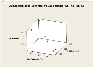
1. OPTIMIZATION OF PROCESS PARAMETERS

It is evident from Table.5 that six values of each independent input parameter have been taken on the basis

of their corresponding least possible values of their squares of residuals. However, two values from each level of input parameters have been drawn corresponding to the lowest possible squares of residuals. Each input factor varies at three levels so (2*3) 6 rows have been selected for each factor optimization and 3D scatter plot have also been drawn as Figures 15(A-F). Single point (out of six points) from each scatter plot has been selected, corresponding to the minimum possible surface roughness and maximum possible MRR. Row wise optimized values may also seen representing in Table.9.

200

1.2 150

1.4 1.6 1.8

40 ₆₀ 100

80

Ra (Microns)

MRR (mg/min)

Gap Voltage Vg (V)

200 1.4

150 1.6

4 1.8

6 ₁₀₀

8

Ra (Microns)

MRR (mg/min)

Dielectric Flush Rate (L/min)

3D Scatterplot of Ra vs MRR vs Flush Rate: HSS T42 (Fig.B)

200

1.2 150

1.4 1.6

1.04 1.8

1.12

1.20 100

1.28

Ra (Microns)

MRR (mg/min)

Spark on time, Ton (micro seconds)

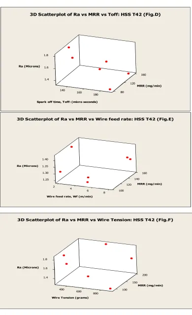
160 1.4

120 1.6

1.8

140

160 80

180

Ra (Microns)

MRR (mg/min)

Spark off time, Toff: (micro seconds)

3D Scatterplot of Ra vs MRR vs Toff: HSS T42 (Fig.D)

160

140 1.25

1.30 1.35

120 1.40

2

4

6 100

8

Ra (Microns)

MRR (mg/min)

Wire feed rate, Wf (m/min)

3D Scatterplot of Ra vs MRR vs Wire feed rate: HSS T42 (Fig.E)

200

150 1.4

1.6 1.8

400 ₆₀₀ 100

800

Ra (Microns)

MRR (mg/min)

Wire T ension (grams)

3D Scatterplot of Ra vs MRR vs Wire Tension: HSS T42 (Fig.F)

2. RESULT

Figures15 (A-F) show the relationship beween individual influencing parameter (Vg, Fr, Ton, Toff, Wf & Wt) and optimized response i.e. surface roughness (Ra) with corresponding values of MRR. Table IX also indicates that unique value of each influencing parameter (corresponding to its serial numbers of table V), which gives optimum

responses, as highlighted. Again the experiment has been conducted on HSS T42 using WEDM by setting the optimum parametric combinations (Vg, Fr, Ton, Toff, Wf & Wt) as 90 (Volt), 6 (Lit./min), 1.05 (S), 190 (S), 5 (m/min) and 900 (grams) respectively and the values of Ra= 1.1462 (m) at MRR=113 (mg/min) have been found.

Table IX

Best parametric combinations and their possible responses

SN Gap

Voltage (Vg)

Flush Rate (Fr)

Spark Time (TON)

Spark Time (TOFF)

Wire Feed (Wf)

Wire Tension

(Wt)

Surface Roughness

(Ra)

Obs.

Surface Roughness

(Ra)

Predicted.

(Residual)2 Material Removal Predicted

(MRR)

Volt Lit./min S S m/ min Grams m m (m)2 mg/min

37 90 6 1.05 130 5 600 1.2334 1.2735 0.001608 111

39 90 6 1.25 130 2 900 1.3286 1.3062 0.000502 105

38 90 6 1.05 160 5 900 1.2158 1.2424 0.000708 109

55 60 6 1.25 190 8 900 1.3682 1.3643 1.52E-05 148

38 90 6 1.05 160 5 900 1.2158 1.2424 0.000708 109

16 90 4 1.15 190 8 900 1.3024 1.3006 3.24E-06 89

3. CONCLUSION

It may be concluded that the model„S1‟ is the best fitted model for material removal rate and surface roughness of HSS T42 on the basis of P-values as shown in Fig.11-13. BPANN modelling technique may be considered as the best modelling tool of surface roughness of HSS T42 under WEDM. From the best modelled training data, optimum parametric combinations i.e. Vg, Fr, Ton, Toff Wf and Wt observed as 90 Volt, 6 Lit./min, 1.05 S, 190 S, 5 m/min and 900 grams respectively and the corresponding value of Ra is 1.1462 m at MRR=113 (mg/min) whereas the average Ra = 1.5965 (m) at MRR = 147 (mg/min). It has been seen that this technique is able to successfully minimize Ra by 28.2% with increase in MRR by 23.12% from its average value on HSS T42. Such combination may be applied for industrial application wherever needed.

REFERENCES

[1] Gatto A., Luliano L., Cutting mechanisms and surface features of WEDM metal matrix composite, Journal of Material Processing Technology 65 (1997) 209-214.

[2] Jaharah A., C. Liang, Wahid A., S.Z., Rahman M., and C. Che Hassan, “Performance of copper electrode in electical discharge machining (edm) of aisi h13 harden steel,” International Journal of Mechanical and Materials Engineering, vol. 3, no. 1, pp. 25–29, 2008.

[3] Bawa, H.S. (2004): Manufacturing Process-II, The McGraw Hill Companies, pp.186-187.

[4] Boothroyd, G.; Winston, A.K. (1989): Non-conventional machining processes, in Fundamentals of Machining and Machine Tools,

[5] Marcel Dekker, Inc, New York, 491.

[6] Montgomery D.C., Design and Analysis of Experiments, Wiley, Singapore, 1991.

[7] Rao G. Krishna Mohana , G. Rangajanardha , Rao D.

[8] Hanumantha , Rao M. Sreenivasa, Development of hybrid model and optimization of surface roughness in electric discharge machining using artificial neural networks and genetic algorithm. journal of materials processing technology 2 0 9 ( 2 0 0 9 ) 1512– 1520.

[9] Gencay Ramjan, Qi Min. Pricing and bedging derivative securities with neural networks : Bayesian regularization, early stopping and bagging. IEEE Trans Neural Networks 2001;12(4): 726-34.

[10] Ho K.H, Newman S.T., Rahimifard, S., Allen, R.D., (2004). State of the art wire electrical discharge machining (EDM) Int J Mach Tools Manuf. 44:1247 – 1259.

[11] I. Puertas, C.J., Lues, A study on the machining parameters optimization of electrical discharge machining, Journal of Material Processing Technology 143-144 (2003) 521-526. [12] Pradhan Mohan Kumar, Chandan Kumar Biswas et al.

Neuro-fuzzy and neural network-based prediction of various responses in electrical discharge machining of AISI D2 steel. Int J Adv Manuf Technol (2010) 50:591–610.

[13] Erzurumlu O., H. T., “Comparison of response surface model with neural network in determining the surface quality of moulded parts,” Materials and Design, vol. 28, no. 2, pp. 459–465, 2007. [14] Panda DK, Bhoi RK (2005) Artificial neural network prediction

of material removal rate in electro-discharge machining. Mater Manuf Process 20:645–672.

[16] Salonitis K, Stournaras A, Stavropoulos P, Chryssolouris G (2009) Thermal modelling of the material removal rate and surface roughness for die-sinking EDM. Int J Adv Manuf Technol 40(3–4):316–323.

[17] Scott,D., Boyina, S., Rajurkar, K.P., 1991 “Analysis and optimization of parameter combination in wire electrical discharge machining.” Int. J. of production research.29 (11) 2189-2207.

[18] Shobert, E.I. (1983): What happens in EDM Electrical Discharge Machining: Tooling, Methods and Applications, Society of Manufacturing Engineers, Dearborn, Michigan, pp.3–4. [19] Tsai, H.C.; Yan, B.H.; Huang, F.H (2003): EDM performance of

Cr/Cu based composite electrodes, International Journal of Machine Tools & Manufacturing, 43, 3, pp.245–252.

Mr. U. K. Vates

Research Scholar- ISM Dhanbad, India) Under Supervision of Dr. N .K. Singh and Dr. R. V. Singh Teaching & Research Experience – 10 years Research Publications - More than 12

Dr. N .K. Singh

Associate Professor (Workshop) ISM Dhanbad Teaching & Research Experience – 25 years Research Publications - More than 28.

Dr. R. V. Singh

Professor and Head Deptt of Mech Engg FET, MRIU, Faridabad

Teaching & Research Experience – 18 years Research Publications - More than 25