www.nat-hazards-earth-syst-sci.net/11/367/2011/ doi:10.5194/nhess-11-367-2011
© Author(s) 2011. CC Attribution 3.0 License.
and Earth
System Sciences
Spatio-temporal avalanche forecasting with Support Vector
Machines
A. Pozdnoukhov1, G. Matasci2, M. Kanevski2, and R. S. Purves3
1National Centre for Geocomputation, National University of Ireland, Maynooth, Ireland 2Institute of Geomatics and Analysis of Risk, University of Lausanne, Lausanne, Switzerland 3Department of Geography, University of Zurich, Zurich, Switzerland
Received: 1 June 2010 – Revised: 14 October 2010 – Accepted: 25 November 2010 – Published: 9 February 2011
Abstract. This paper explores the use of the Support Vector Machine (SVM) as a data exploration tool and a predictive engine for spatio-temporal forecasting of snow avalanches. Based on the historical observations of avalanche activity, meteorological conditions and snowpack observations in the field, an SVM is used to build a data-driven spatio-temporal forecast for the local mountain region. It incorporates the outputs of simple physics-based and statistical approaches used to interpolate meteorological and snowpack-related data over a digital elevation model of the region. The interpretation of the produced forecast is discussed, and the quality of the model is validated using observations and avalanche bulletins of the recent years. The insight into the model behaviour is presented to highlight the interpretability of the model, its abilities to produce reliable forecasts for individual avalanche paths and sensitivity to input data. Estimates of prediction uncertainty are obtained with ensemble forecasting. The case study was carried out using data from the avalanche forecasting service in the Locaber region of Scotland, where avalanches are forecast on a daily basis during the winter months.
1 Introduction
Snow avalanches are of particular interest as natural hazards because of the complex non-linear relationship with meteorological conditions, topography and a wide variety of other factors including human activity as triggers for the events (McClung and Schaerer, 1993). Local avalanche reports provide regular assessments of current, and forecasts
Correspondence to: A. Pozdnoukhov
of future, snowpack stability for regions which are typically considered to be homogeneous with respect to the primary influences on avalanche activity. Textual forecasts are often accompanied by a schematic map and may include detailed information on snowpack formation and its instabilities for particular aspects and altitudes.
Numerical methods used to assist in avalanche forecasting range from complex systems involving physical models (Durand et al., 1999; Lehning et al., 1999) to various heuristic and statistical decision-support methods (Schweizer and F¨ohn, 1996; Keiler et al., 2006; Bolognesi, 1993). Statistical methods of avalanche forecasting link several available input variables (meteorological factors, snowpack properties and stability factors as identified by LaChapelle (1980) to the target outputs. However, the choice of the target is not evident. Although the verified avalanche hazard might be seen as an ideal choice (Schweizer and F¨ohn, 1996), forecasted avalanche hazard is much more commonly available (Brabec et al., 2001). Many approaches have used observations of avalanche activity as a target and assumed that it is related to avalanche hazard (Buser, 1989; Heierli et al., 2004). However, this relationship is not always obvious, particularly for low hazard levels and where observations are missing, for example in stormy conditions (Schweizer et al., 2003).
A few examples of more localised forecasting methodologies have been produced, typically with the aim of forecasting for individual avalanche paths (McCollister et al., 2003; Bolognesi, 1993).
The Nearest Neighbours approach is a popular decision support tool due to its simplicity and apparent interpretability by practitioners in operational use (Buser, 1989; Gassner and Brabec, 2002; Purves et al., 2003; Heierli et al., 2004). The method identifies similar conditions in the past to predict if avalanching is probable in the current day. It can also list the most similar individual past events from the database under these conditions and plot them on the map. These practices accord well with conventional inductive avalanche forecasting processes (LaChapelle, 1980; Purves et al., 2003). The spatialisation of the forecast is left to the practitioner to interpret by examining the neighbours (either textually or on a map) or the forecast output may be classified according to aspects and altitudes as in the Safran/Crocus/Mepra approach of Durand et al. (1999). In forecasts provided by avalanche warning services such detail is provided in the text where hazardous aspects and altitudes are outlined and snow conditions therein are described based on forecaster’s experience and regular fieldwork.
In terms of data availability relevant to avalanche fore-casting, high spatio-temporal resolutions capabilities already exist, in the form of high-resolution digital terrain models and continuous advances in environmental monitoring network technologies able to provide meteorological data (Hart and Martinez, 2006). Snowpack formation models have been developed (Lehning et al., 1999) and significantly advanced over the recent years (Lehning et al., 2006). In the temporal domain, there is substantial evidence that the modelled snowpack conditions can be helpful in predicting avalanche hazard (Lehning et al., 2006; Schirmer et al., 2009).
Given that these data are available, an attempt can be made to develop an exploratory data-driven system to assist in spatio-temporal forecasting of the avalanche activity. This paper presents the results of such developments, targeting avalanches on Ben Nevis and the surrounding mountains in the Lochaber region of Scotland. Natural avalanche activity in the region is mainly the result of heavy snowfalls and associated high winds as a consequence of a maritime climate together with rapid temperature changes. Human-triggered avalanches are common as well as the area is a popular winter climbing venue. Weather reports and local avalanche forecasts are produced daily in winter months by the sportscotland Avalanche Information Service (SAIS) in the area1. In this paper we report on the use of a Support Vector Machine (SVM), a promising non-parametric classification method for exploratory data analysis and predictive modelling of snow avalanches. The study extends the results of Pozdnoukhov et al. (2008) in which SVM was
1http://www.sais.gov.uk/
applied to a purely temporal problem of predicting the days when avalanches are probable at the site. In this work, we demonstrate how similar data-driven methodology is applied to produce spatialised forecasts of avalanche activity.
The paper is organized as follows. First, in Sect. 2.1, we introduce data-driven classification as an approach to decision support in avalanche forecasting. Next we present the basic features of a particular machine learning classification method, SVM. In Sect. 3, the raw data description and the generated features are introduced, the classification model is set up and model parameters are tuned. Section 4 describes and discusses the obtained results on the application of SVMs for spatio-temporal avalanche forecasting in terms of its ability to predict avalanche events and provide spatial danger maps. Section 5 provides an insight into the interpretability of the obtained forecasts, discusses the sensitivity to input parameters and estimates the prediction uncertainties. Section 6 concludes the paper by resuming the main results and issues raised by this work.
2 Predictive statistical learning from data
2.1 Forecasting as spatio-temporal classification
A wide range of numerical models and tools have been developed over the last decades to support decision making processes in environmental applications ranging from physical models, through expert systems, to a variety of statistically-based methods. In operational forecasting a mixture of all three approaches is often used, with process chains involving physical models and statistical or expert systems being relatively common (Durand et al., 1999; Purves et al., 2003; Bolognesi, 1993; Schweizer and F¨ohn, 1996).
Since availability of real time spatially distributed data describing a wide range of parameters has increased through technological advances in sensor networks and automated environmental monitoring (Hart and Martinez, 2006), we can expect data-driven models to become increasingly important. Robust adaptive tools are required that can explore incoming volumes of information, extract useful knowledge suitable for visualization and predict observed dependencies hidden in data without making restrictive assumptions about data generating mechanisms (Breiman, 2001). Such tools are provided by the emerging field of statistical machine learning (Hastie et al., 2001). One of the fundamental problems studied in Statistical Learning Theory (Vapnik, 1998) is that of binary classification. This problem can be stated as the identification of a decision rule discriminating the data into two classes (such as “dangerous” and “safe”) based on available empirical samples.
dataset might contain samples with identical conditions (with respect to the registered meteorological and snowpack parameters) which either led to an avalanche event or not. In other words, in the input space of factors the “dangerous” and “safe” classes overlap, hence there is no hard decision boundary between those conditions. The requirements for a classifier to provide useful decision boundaries include its ability to discover non-linear solutions, soft treatment of input data that allows misclassifications of observed data samples (either misses or false alarms) and, consequently, an associated confidence measure. Moreover, it is necessary to provide a variety of ways to enhance interpretability of forecasts. In this paper we apply a powerful data-driven classifier, the Support Vector Machine, which matches the above mentioned requirements, and discuss its use in decision support for avalanche forecasting.
2.2 Support Vector Machine
SVM is a machine learning approach derived from Statistical Learning Theory aimed to deal with data of high dimensionality by approaching nonlinear classification problems in a robust and non-parametric way (Vapnik, 1998; Sch¨olkopf and Smola, 2002). Here we describe the main principles of SVMs which have important implications for their application in decision-oriented avalanche forecasting.
Firstly, suppose one deals withN linearly separable data samples(x1,y1),...(xN,yN), wherexare the input features
(independent variables) and y∈ {+1,−1} are the binary labels. “Linearly separable” data can be discriminated into two classes by a hyperplane. The idea of SVM is to separate this dataset by finding the hyperplane that is the farthest apart from the closest training points of each class. The minimal distance between the hyperplane and the training points, which is maximized by the SVM algorithm, is called the margin. The decision function used to classify the data is linear, as follows:
f (x,{w,b})=w·x+b, (1) where the vector w and a threshold constant b define the orientation of the separating hyperplane. The binary decisions are taken according to the sign(f (x)). Parameters {w,b}are optimized in order to maximize the margin, which is inversely proportional to kwk2. This is a quadratic optimization problem with linear constraints which has a unique solution. Moreover,wis a linear combination of the training samplesxi, many of them having zero weightsαi:
w=
N X
i=1
yiαixi. (2)
The samples with non-zero weights are the only ones which contribute to the maximum margin solution. They are the closest samples to the decision boundary and are called the Support Vectors. This simple classifier is then extended
to account for overlapping data and presence of noisy or mislabelled samples such that a misclassification of the training samples is allowed. A cost hyper-parameter C
is introduced in the optimization in order to control the trade-off between the maximization of the margin and the permitted training errors.
Then, the so-called “kernel trick” is used to produce non-linear decision boundaries. The kernel is a symmetric semi-positive definite functionK(x,x0). According to the Mercer theorem this function corresponds to a dot product in some space (Reproducing Kernel Hilbert Space, RKHS). By substituting the dot products with kernel functions a linear method is transformed into a nonlinear one. This is the case for linear SVM, where the decision function (1) relies only on the dot products between samples. Omitting the optimization problem, which is solved numerically to optimize the weights,αi, the final classification model takes
the form of a kernel expansion:
f (x)=
N X
i=1
yiαiK (x,xi)+b . (3)
Typical kernels are Gaussian RBFs,K(x,x0)=e−( x−x0)2
2σ2 ,
which value decays with distance between samples thus leading to a simple interpretation of (3) as of weighted combination of “similar” samples. The bandwidth parameter
σ of the kernel must be tuned using cross-validation or a testing dataset.
It has been shown in Statistical Learning Theory that the maximum margin principle prevents over-fitting in high-dimensional input spaces, thus leads to good generalization abilities and accurate predictions (Vapnik, 1998). Theoretical difficulties faced by conventional nearest neighbours ap-proaches when applied to high-dimensional datasets (Beyer et al., 1999) have been previously observed in avalanche forecasting applications (McCollister et al., 2003).
2.3 Interpretation for decision support
SVM is specifically constructed to solve a binary classi-fication task and provides hard {+1,−1} decisions. It is however possible to associate a smooth confidence measure,
p:0< p(y= {+1,−1}|x) <1 to characterize an uncertainty in classification based on the values of the decision function (1) or (3). This is usually done by taking a sigmoid transformation off (x)(Platt, 1999):
p(y=1|x)= 1
(1+exp(a·f (x)+b)), (4)
whereaandbare constants. The value ofais negative, and if
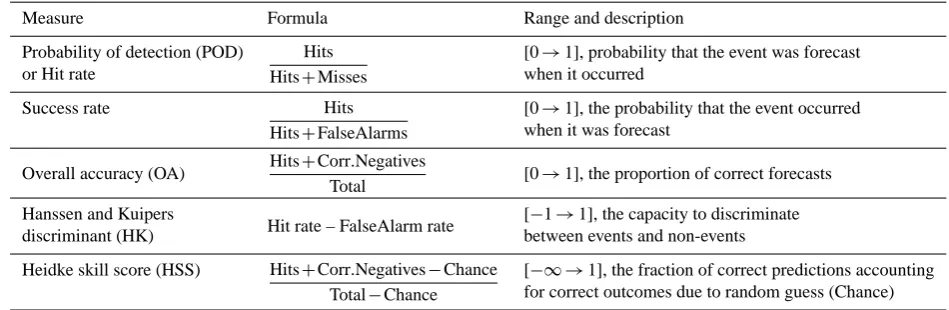
Table 1. Forecast verification measures and skill scores (Doswell et al., 1990; Wilks, 1995).
Measure Formula Range and description
Probability of detection (POD) Hits
Hits+Misses
[0→1], probability that the event was forecast
or Hit rate when it occurred
Success rate Hits
Hits+FalseAlarms
[0→1], the probability that the event occurred when it was forecast
Overall accuracy (OA) Hits+Corr.Negatives
Total [0→1], the proportion of correct forecasts
Hanssen and Kuipers
Hit rate – FalseAlarm rate [−1→1], the capacity to discriminate
discriminant (HK) between events and non-events
Heidke skill score (HSS) Hits+Corr.Negatives−Chance
Total−Chance
[−∞ →1], the fraction of correct predictions accounting for correct outcomes due to random guess (Chance)
smooth confidence outputs which may later be tuned to optimize the desired forecast quality measures. Empirical evidence suggests that (4) can be used to provide an estimate of class-conditional posteriors (Platt, 1999) if calibrated by maximizing the likelihood (the negative log-likelihood to simplify the optimization) on the testing dataset.
The output of the binary classification system can be characterized by several basic measures computed from the contingency table. Concerning natural hazards, different possible forms and interpretations of the forecast are usually considered. Firstly in categorical forecasts a decision boundary is directly used to classify the region/time as being either dangerous or not. The Table 1 provides some conventional forecast quality measures used to assess the forecast quality. These measures are used here to tune the hyper-parameters of SVM and the decision threshold. Secondly, in probabilistic forecasts the output of the system can be interpreted as a continuous measure of the likelihood of an event in the temporal or spatio-temporal domain of the forecast. Such forecasts can be used, for example, for risk assessment. Thirdly, a so-called descriptive forecast is often desirable, since experts wish to interpret and incorporate, for instance, a detailed list of similar events into their decision-making process. Concerning the last category, the Nearest Neighbours methods and their variations commonly named as the “methods of analogues” are extensively used (Heierli et al., 2004). In a temporal domain (forecasting days with avalanching) Support Vector Machines can produce all of the above forms of forecasts (Pozdnoukhov et al., 2008).
In the spatio-temporal domain a categorical forecast is simply the predicted class, however, the probabilistic inter-pretation for predicting the event probability is complicated due to very low base rates of events at individual avalanche paths. As insufficient data are available to calibrate probabilistic post-processing for individual locations, (4) can be used to provide a confidence measure associated with binary prediction and helpful in assessing the likelihood of an
avalanche event at a certain location under certain conditions. The situation is also complicated by the fact that a triggering mechanism is usually known only for events which were directly observed, deliberately triggered, or reported by those who triggered them. To facilitate interpretation, descriptive forecasts can be produced by providing the corresponding Support Vectors which are the most valuable discriminating events in the past related to current conditions. Below, these ideas are explored in detail showing how the data-driven SVM classifier can be exploited for exploratory analysis of avalanching datasets and interpreted for decision support in spatio-temporal forecasting.
3 Spatio-temporal forecasting with SVM
3.1 Avalanche forecasting in Lochaber region
Avalanche forecasts are produced daily in the Lochaber region of Scotland, and the Nearest Neighbour-based system called CORNICE is currently used in decision support (Purves et al., 2003). The original data on weather conditions in the region consist of daily measurements of 9 meteorological and snowpack variables starting from the winter season of year 1991. The list of the available variables is presented in Table 2, along with the class/category that each variable is assigned to according to the scheme proposed in (LaChapelle, 1980) (class I – slope stability factors, class II – snowpack factors and class III – meteorological factors).
Table 2. List of the 9 meteorological and snowpack variables recorded daily in the winter season.
Variable Class Description
Snow index III Ordinal index (0–10) of the precipitation as fresh snow on the day
Rain at 900 m III Binary variable indicating if rain is falling at 900 m (“1” value, “0” otherwise)
Snow drift II Binary variable taking “1” values when sufficient snow drifting is observed (“0” otherwise)
Air temperature III Midday air temperature at the automatic weather station measured in◦C
Wind speed III 24 h vector mean speed from the automatic weather station reported in m s−1
Wind direction III 24 h vector mean wind direction from the automatic weather station reported in◦
Cloud cover III Cloud cover as percentage of the sky
Foot penetration II Penetration of the foot in the snow measured in cm at the pit site by forecasters
Snow temperature II Snow temperature at a depth of 10 cm at the pit site measured in◦C
Legend
Gully B
0 500 1,000 1,500 Meters Gully A
Other gullies
Fig. 1. The hillshade of the DEM of the Lochaber region and
locations of the gullies where avalanches are typically observed. Two particular gullies used to illustrate some properties of developed predictive system throughout the paper are marked with A (“No. 3 Gully” on Ben Nevis face) and B (“The Chancer” on Aonach Mor).
Avalanches are observed mainly in 49 gullies and slopes on north to east facing aspects. The locations of these events is shown in Fig. 1 along with a hillshade representation of the SRTM Digital Elevation Model (DEM) of the region. Computations were carried out using a 10 m DEM available through the National Mapping Agency. The avalanche and weather data were partitioned into a training period from 1991–2005, while the winters of 2006–2008 were used for validation only.
3.2 Data preparation: conditioning factors
The binary classification problem was formulated to delineate the conditions in space and time that led to observed avalanche activity. The input feature vectors were composed of several groups of factors for every location in space-time. The idea behind this process is to generate discriminative predictants related to avalanche activity. However it is evident that the sets of samples of safe conditions and avalanche events overlap in every space of conditioning factors as no triggering mechanism is incorporated in modelling.
The inputs have to be generated both for every historical observation to train and validate the model and for every space-time location provided for prediction. Thus, in order to produce a spatial danger prediction map for a particular day these attributes have to be precomputed for every spatial location on the grid covering the region. Each cell in the 10 m resolution grid will be described by the conditioning factors computed for that location for the considered day. The SVM model then predicts the avalanche danger by assigning a decision function value (tuned in the [0, 1] interval) to each one of these points.
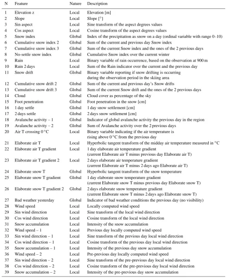
The conditioning factors provided to the model are described hereafter and the complete set of 39 features is listed in Table 3.
3.2.1 Global meteorological and snowpack factors
Table 3. List of the 39 input features (predictors).
N Feature Nature Description
1 Elevation z Local Elevation [m]
2 Slope Local Slope [◦]
3 Sin aspect Local Sine transform of the aspect degrees values
4 Cos aspect Local Cosine transform of the aspect degrees values
5 Snow index Global Index of the precipitation as snow on a day (ordinal variable with range 0–10)
6 Cumulative snow index 2 Global Sum of the current and previous day Snow index
7 Cumulative snow index 3 Global Sum of the current Snow index and the ones of the 2 previous days
8 No-settle snow index Global Cumulative Snow index over the current winter
9 Rain Local Binary variable of rain occurrence, based on the observation at 900 m
10 Rain 2 days Local Sum of the Rain indicator over the current and the previous day
11 Snow drift Global Binary variable reporting if snow drifting is occurring
during the observation period in the skiing area
12 Cumulative snow drift 2 Global Sum of the current and previous day’s Snow drifts
13 Cumulative snow drift 3 Global Sum of the current Snow drift and the ones of the 2 previous days
14 Cloud Global Cloud cover as percentage of the sky
15 Foot penetration Global Foot penetration in the snow [cm]
16 1 day settle Global 1 day snow settlement [cm]
17 2 days settle Global 2 days snow settlement [cm]
18 Avalanche activity – 1 Global Indicator of global avalanche activity the previous day in the region
19 Avalanche activity – 2 Global Sum of Avalanche activity over the 2 previous days
20 Air T crossing 0◦C Local Binary variable indicating if the air temperature is
rising above 0◦C from the previous day
21 Elaborate air T Local Hyperbolic tangent transform of the midday air temperature measured in◦C
22 Elaborate air T gradient Local 1 day elaborate air temperature gradient
(current Elaborate air T minus previous day Elaborate air T)
23 Elaborate air T gradient 2 Local 2 days elaborate air temperature gradient
(current Elaborate air T minus 2 days ago Elaborate air T)
24 Elaborate snow T Global Hyperbolic tangent transform of the snow temperature
25 Elaborate snow T gradient Global 1 day elaborate snow temperature gradient
(current Elaborate snow T minus previous day Elaborate snow T)
26 Elaborate snow T gradient 2 Global 2 days elaborate snow temperature gradient
(current Elaborate snow T minus 2 days ago Elaborate snow T)
27 Bad weather yesterday Global Indicator of bad weather conditions the previous day (no visibility)
28 Wind speed Local Locally computed wind speed
29 Sin wind direction Local Sine transform of the local wind direction
30 Cos wind direction Local Cosine transform of the local wind direction
31 Snow accumulation Local Intensity of the snow accumulation
32 Wind speed – 1 Local Previous day locally computed wind speed
33 Sin wind direction – 1 Local Sine transform of the previous day local wind direction
34 Cos wind direction – 1 Local Cosine transform of the previous day local wind direction
35 Snow accumulation – 1 Local Intensity of the previous day snow accumulation
36 Wind speed – 2 Local Pre-previous day locally computed wind speed
37 Sin wind direction – 2 Local Sine transform of the pre-previous day local wind direction
38 Cos wind direction – 2 Local Cosine transform of the pre-previous day local wind direction
39 Snow accumulation – 2 Local Intensity of the pre-previous day snow accumulation
measurement was held constant over the entire region after a hyperbolic tangent transformation to obtain an increased sensitivity when approaching the 0◦C melting point (Gassner
2 previous days were also computed. A similar procedure has been adopted for the global variable of foot penetration, where the differences between the actual and previous day’s value have been integrated in the feature vector. These derived “expert features” were constructed in a dialogue with a local avalanche forecaster who was asked to list important indicators of avalanche activity.
3.2.2 Spatially variable terrain features and meteorological factors
The spatial features comprise topographical characteristics directly available from avalanche observations and the DEM: they consist of the elevation, slope and aspect of each spatial location. Then, in order to model the local avalanche-related conditions to produce the spatially variable forecast, the series of daily measurements of meteorological conditions related to snowpack stability have to be interpolated over the region taking into account the terrain.
The air temperature measured by the automatic weather station located at an altitude of 900 m was interpolated by means of a constant temperature/elevation gradient of 0.65◦C/100 m (Barry, 1981). Then, as suggested in
(Gassner and Brabec, 2002), a hyperbolic tangent transform was applied to emphasize the critical 0◦C transition. Temperature inversion and local orographic effects were not considered.
Wind fields for a constant wind speed of 10 m s−1 and directions 0◦−350◦ were precomputed following the MicroMet model (Liston and Elder, 2006). The model is linear with respect to the wind speed and the modelled wind fields can be easily adjusted according to the observations on a particular day. Wind direction was included in the feature vector as N-S and W-E components for the current and 2 previous days
Snowpack variability in space was taken into account by considering a snow mass balance index given by the observed snowfall intensity (Snow index>0) and the influence of snow drifting (Snow drift = 1) governed by the precomputed wind fields. A spatially varying variable indicating the snow accumulation at a given location was computed and included in the feature vector for the current and the 2 preceding days. Ablation was not considered.
Rainfall is recorded as a binary variable at an altitude of 900 m – this was spatialised using current temperature and elevation over the whole region. Thus, the binary variable rain was transformed into a continuous one with a hyperbolic tangent transformation to incorporate the smooth snow-to rain melting transition. The rain descriptor for the preceding day was also included in the feature vector.
The presented approach can be seen as a relatively “naive” approach to modelling local meteorology and snowpack that could be substituted by a more comprehensive physical model such as, for example, Alpine3D (Lehning et al., 2006). While the results of such efforts would be of great interest,
the described simplified system appears to be useful for extracting the dependencies between indirect factors and avalanche activity as long the consistency of the data used for training and the prediction is kept.
The final input vector contained 39 features: 22 spatio-temporal features (describing local conditions at a given grid cell) and 17 temporal conditioning factors of global validity (constant over the region).
3.3 The spatio-temporal classification problem
While it was relatively straightforward to put the registered avalanche events into a dataset as the class entities representing avalanche events (with labely= +1), it is much harder to describe the set of the “safe” conditions (y= −1). Here lies an important issue – the samples of the “safe” class have to bring discriminative information. In other words, to include a sample of the “safe” class one has to be sure that the snowpack at the given slope is stable under given conditions, while still representing a “non-trivial” data sample. The “safe” samples were constructed by combining the spatial features of potential avalanche paths and the meteorological conditions on days with good visibility when no avalanche events were observed. One can, however, expect many false alarms types of errors produced by a classifier from these samples, as avalanches could have been triggered in some of these gullies by climbers. Then, several low-elevation and flat slope locations (where no avalanche events were ever observed) were included in the “safe” subset to enrich this set.
For the training set, this approach resulted in 606 posi-tively and 89 335 negaposi-tively labelled samples while for the validation set we obtained 106 positively and 5780 negatively labelled samples. The problem is thus very unbalanced. Modification of the misclassification costs of the different classes is usually suggested (Lin et al., 2000) when applying SVM in such cases. An equivalent approach is to introduce virtual samples into the dataset. This was done by generating virtual “avalanche cases” whose input features were normally distributed around the real cases within the
range of observation uncertainty and/or instrumental error.
Particularly, the slope, aspect (usually registered from visual observations and thus related to considerable uncertainty), air temperature, snow temperature, wind speed and direction including the ones for preceding days were sampled to produce 25 virtual samples for every real avalanche case. The resulting training set consisted of 15 756 positive and 89 335 negative cases. The validation set consisted of 2756 positives and 5780 negative cases. Data preparation is an inevitable source of model uncertainty that will be described in Sect. 5.3 in more detail.
Table 4. SVM model: contingency tables for training and validation
datasets. Numbers in brackets refer to real events.
Predicted
Class +1 Class−1
(a) Training set fitting
Actual Class +1 14131 (545) 1625 (61)
Class−1 3907 85 428
(b) Validation data prediction
Actual Class +1 2541 (97) 215 (9)
Class−1 1150 4630
and the triggering of avalanches depends on other parameters (such as the quality of climbing available). In cases where more complete data are available (e.g. McCollister et al., 2003 where individual avalanche paths were actively observed within a ski area) it may be that there is less need to generate virtual samples.
3.4 Tuning of parameters
The proper choice of the hyper-parameters of the classifier is crucial to avoid overfitting and produce a model with predictive abilities. The parameters of the classifier were tuned by considering the HK discriminant, HSS and OA measures (see Table 1 for details) computed on a separate testing subset consisted of 20% of the data randomly chosen from the training dataset. The comprehensive choice over the parameter space (σ andC) and the thresholds resulted in the following values: σ=10, C=0.5. The parameters of the sigmoid transform (4) were found to be a= −1.2,
b= −0.23 and the decision function threshold t (tuned on the p(y=1|x) values) was set at 0.37. The contingency table for the training set is shown in Table 4a. The chosen model misclassifies many “safe” samples and misses 61 observed avalanche cases illustrating highly overlapping data. The choice of the hyper-parameters is another source of uncertainty that will be taken into account below in Sect. 5. 4 Results, validation and discussion
4.1 Avalanche events prediction
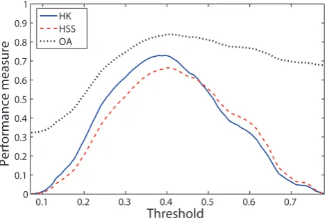
The trained SVM model was used to forecast the validation data of the 2006–2007 and 2007–2008 winter seasons. Performance curves are presented in Fig. 2, and the exact values for the chosen decision threshold can be found in Table 4b. The obtained performance measures are: POD = 0.92, OA = 0.84, Success rate = 0.69, HK = 0.72, HSS = 0.66. For the two validation seasons, 97 of the 106 avalanches of the season were predicted at the cost of 1150 false alarms (9 days per season on average).
0.1 0.2 0.3 0.4 0.5 0.6 0.7
0 0.1 0.2 0.3 0.4 0.5 0.6 0.7 0.8 0.9 1
Threshold
Performance measure
HK HSS OA
Fig. 2. Performance curves (HK, HSS, OA) computed on the
validation data set. The decision thresholdt pre-selected on the
testing set is 0.37.
Table 5. Nearest Neighbours model: contingency table for the
validation dataset. Numbers in brackets refer to real events.
Predicted
Class +1 Class−1
Actual Class +1 1415 (55) 1341 (51)
Class−1 827 4953
To assess the performance of an SVM in comparison with a conventional benchmark method, a Nearest Neighbours classifier was applied to the dataset. One classic approach in forecasting is to treat a day as an avalanche day if 3 or more of the 10 nearest neighbours of the sample under consideration are avalanche releases (Buser, 1989) was found to be sub-optimal for this dataset. After a wide search, the best results have been obtained with a model taking into account 20 neighbours and forecasting an avalanche if 2 or more were positive examples. The predictions on the validation set for the retained model are summarized in Table 5. In this case, the performance scores take the following values: POD = 0.51, OA = 0.75, Success rate = 0.63, HK = 0.37, HSS = 0.39. These results are comparable with those typically obtained for applications of NN, with for example (Heierli et al., 2004) reporting values of POD = 0.73, OA = 0.73, Success rate = 0.39, HK = 0.34, HSS = 0.42 for forecasting in the same area as a binary (i.e. avalanche day/no avalanche day) problem.
is an unavoidable consequence of a well trained classifier where there is a pronounced overlap between classes as discussed above. Indeed, these false alarms are likely to be indicative, at least in some cases, of conditions where avalanching might have occurred if a trigger was available (i.e. they might simply indicate that little back country activity was carried out on the day in question). If compared with the NN approach, less events are missed by SVM (9 with SVM vs. 51 with NN). This translates to a high POD, revealing thus a good ability in the detection of the critical situations resulting in an avalanche release at a given path. The other performance measures show a similar trend with relevant differences between the two models. However, it is important to note that these results are for a single region, with a low base rate, and for areas with more data with respect to avalanche events (e.g. McCollister et al., 2003) performance of the NN method may improve.
Nonetheless, by contrast to our previous work (Pozd-noukhov et al., 2008) where the improvements in forecasting performance over traditional NN for temporal forecasts were less marked, we see a large improvement here. This suggests that when the target variable (now an avalanche in a specific location, rather than an avalanche in a region) is more specific, the ability of SVMs to effectively partition a high-dimensional space is more important.
4.2 Danger maps evaluation
An example of a produced forecast is presented in Fig. 3. The map illustrates the outputs of the model, rescaled according to Eq. (4), computed at a resolution of 10 m for one day in the validation period (15 February 2007). On that day 3 avalanches were observed and the produced danger map highlights in the regions where the events occurred. However, the validation or evaluation of this kind of prediction is not an evident task as a complete ground truth is unknown (missing avalanching conditions over the entire map extent). One possible approach is to relate it to the avalanche hazard bulletins produced by a human forecaster. The bulletin for 15 February 2007 is provided as an example: “The freezing level rose to above the summits and rain fell.
The top layer of the windslab that formed on Tuesday night is now very wet. Around midday the deeper layers of this snow remained sub-zero and dry. Easy shears were observed both between the wet and the dry snow, and between the dry snow and the old hard snow-ice. Avalanches have occurred where deep deposits of this windslab are found. This is generally on North to East aspects above 1000m. The avalanche hazard is High (Category 4). Cornices are liable to spontaneous collapse in the mild, wet conditions.” The map produced
appears to broadly represent this description of the actual avalanche hazard as described by a forecaster. However, it is questionable as to whether such a map is a useful means of describing avalanche danger to individuals.
/
0 500 1,000 1,500Meters
Legend
Avalanches of 15.02.2007 Avalanche danger
Value
High : 0.79 Low : 0.07
Fig. 3. Map of the avalanche danger prediction for 15 February
2007. The avalanche events observed that day are marked with white circles.
60
240
30
210
0
180 330
150 300
120
270 1350 1350 90
Aspect [°]
Elevation [m]
Avalanche danger
1150 1150
950 950
750 750
550 550
350 350
150 150
0
0.1 0.2 0.3 0.4 0.5 0.6 0.7
min = 0.07 max = 0.79
Fig. 4. Aspect/elevation diagram of the avalanche danger prediction
for 15 February 2007.
One method of summarising the variability in avalanche danger is through the use aspect/elevation diagrams, such as are in use by a number of avalanche forecasting services. Typically, these are produced by the forecaster selecting a range of elevations and aspects and shading these appropriately.
26.12.2006 05.01.2007 15.01.2007 25.01.2007 04.02.2007 14.02.2007 24.02.2007 06.03.2007 16.03.2007
0 0.1 0.2 0.3 0.4 0.5 0.6 0.7 0.8 0.9 1
Date
Avalanche danger
Profile of avalanche path B Profile of avalanche path A Event at path A
Event at path B Event in the region
06.01.2007 14.02.2007 03.03.200707.03.200709.03.200713.03.2007
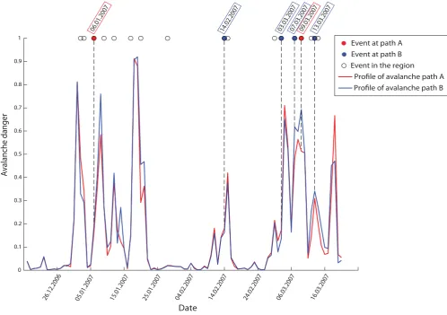
Fig. 5. Evolution of avalanche danger for gullies A and B during the winter season of 2006–2007.
Fig. 3. Here, we can see that the southeast slopes appear to be primarily in one area of high danger east of the avalanche events recorded on that day. The diagram itself might also provide a potential tool for use in presenting information to the public, which links more directly to a textual forecast, though it is important to note that no normalization for the actual distribution of elevation/aspect in the region has been carried out.
4.3 Time series for fixed spatial location
Here we illustrate how the derived model behaves in producing forecasts for individual avalanche paths. The time series of predicted danger (SVM output rescaled in the [0, 1] interval according to (4)) for the two avalanche paths indicated in Fig. 1 is presented in Fig. 5 for a validation period of winter 2006–2007. The avalanche path labelled with “A”, is “No. 3 Gully” found on the east side of Ben Nevis at 1180 m with an aspect of 58◦ and a slope of 45◦, whilst “B”, is “The Chancer” found on the east side of Aonach Mor at 1170 m, with a similar aspect (= 60◦) but at
lower slope (= 34◦). Avalanche events observed in the gullies
are shown with coloured dots, and days with avalanche activity registered elsewhere are marked as white circles.
The forecasts demonstrate different temporal behaviour (for some periods gully A is predicted to be more dangerous than B and vice versa) while both series follow a common pattern which is not surprising for a localized mountain region. The pattern appears to account for the overall hazard in the area and matches well the actual general avalanche activity shown with black circles. However, more detailed validation of the behaviour of the individual avalanche paths is difficult and requires consideration of factors other than the avalanches actually reported since avalanche release on a particular path is an event with a low base rate which complicates introducing a quantitative validation measure.
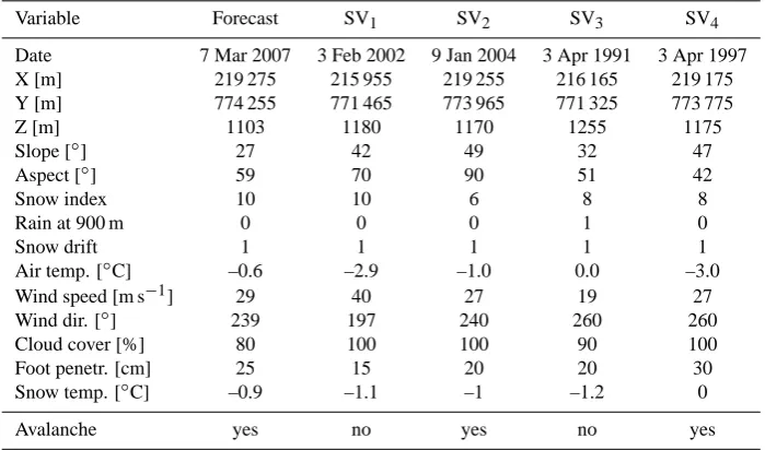
Table 6. Descriptive interpretation of the forecast for a particular location-conditions is provided with the closest Support Vectors: the 4 most
relevant historical reference situations found by the SVM model for the current “Forecast” are listed in columns “SV1” to “SV4”.
Variable Forecast SV1 SV2 SV3 SV4
Date 7 Mar 2007 3 Feb 2002 9 Jan 2004 3 Apr 1991 3 Apr 1997
X [m] 219 275 215 955 219 255 216 165 219 175
Y [m] 774 255 771 465 773 965 771 325 773 775
Z [m] 1103 1180 1170 1255 1175
Slope [◦] 27 42 49 32 47
Aspect [◦] 59 70 90 51 42
Snow index 10 10 6 8 8
Rain at 900 m 0 0 0 1 0
Snow drift 1 1 1 1 1
Air temp. [◦C] –0.6 –2.9 –1.0 0.0 –3.0
Wind speed [m s−1] 29 40 27 19 27
Wind dir. [◦] 239 197 240 260 260
Cloud cover [%] 80 100 100 90 100
Foot penetr. [cm] 25 15 20 20 30
Snow temp. [◦C] –0.9 –1.1 –1 –1.2 0
Avalanche yes no yes no yes
known problem in avalanche forecasting – verifying conditions at the scale of individual slopes, which are known to vary considerably, without observations of these slopes. One potential approach to consider this issue in a spatialised forecast such as that presented here would be to also consider the likelihood of a) avalanches being observed (for example, is the area frequented by mountain guides who regularly report events) and b) avalanches being triggered (how frequently is the slope actually used). Developments such as those implemented by Suter and Harvey (2009), allowing the use of mobile systems for real time reporting of avalanches may go some way to mitigating this data gap in the future.
5 Interpretability and uncertainty
Data-driven methods, such as SVMs, are often criticised for being “black-boxes”. This section addresses this issue by, firstly, providing descriptive forecasts, secondly, by looking at the behaviour of the SVM model when specific changes in weather conditions occur, and thirdly, estimating the forecast uncertainty with a computational Monte Carlo approach by running an ensemble of predictive models.
5.1 Support Vectors as reference events
One reason for the popularity of Nearest Neighbours approaches is due to their ability to provide the reference avalanche events in the past that are most related to the current conditions (Buser, 1989; Gassner and Brabec, 2002; Purves et al., 2003; Heierli et al., 2004). A forecaster
provided with this information has more insight while producing an avalanche bulletin, and the descriptive nature of the information corresponds well with the inductive process of avalanche forecasting. The SVM-based model (3) is essentially a weighted linear combination of the kernel functions and thus provides similar functionality. For every forecast location-conditions inputxf, the historical samples
xi are ordered according to their influenceαiK(xf,xi)and
a predefined number of the most influential events can be provided.
Table 6 provides an example of 4 reference events and their original attributes for a prediction point located in the gully labelled B (“The Chancer”) in Fig. 1 on 7 March 2007. These input conditions for a larger number of Support Vectors can be visualized in a parallel coordinates plot, as implemented for example in (Purves et al., 2003). However it has been observed that the exact nearest neighbours in high-dimensional spaces are relatively meaningless (Beyer et al., 1999; McCollister et al., 2003). Theoretical analysis of Vapnik (1998) suggests that Support Vectors produced by SVM present more meaningful samples for robust discrimination of data in high-dimensional spaces, thus providing a tool to retrieve historical records from a data base of observed events which are the most discriminative and relevant for a particular prediction case.
By comparing the weather/snowpack measurements and terrain features of these situations similar conditions can be noted. For example, all locations on these days in the Support Vectors are associated with new snow and snow drifting, and winds are generally from between south and west, while the avalanche paths lie between east and north-east and are all over 1000 m, which fits well with the relatively mild air temperatures of between –3.0 and 0.0◦C.
Such information is potentially useful to the forecaster especially since it is argued that SVMs provide more discriminating Support Vectors than NN.
5.2 Sensitivity to input conditions
Another important insight into the produced forecast can be provided by exploring its variation with respect to varying input conditions. This helps to quantify the irreducible uncertainty related to measurement errors and the uncertainty of the input conditions inferred from the weather forecasts if these are used operationally as model inputs. This sensitivity analysis is important to investigate if model behaviour coincides qualitatively with forecaster’s expectations. 5.2.1 Decision function analysis
It is possible to derive an analytical estimate of the sensitivity of the decision function to small variations of the individual input parameters. Assuming the individual input features are independent, the partial derivative of f (x)with respect to variablexkfor a Gaussian RBF kernel-based model is given by:
∂f (x) ∂xk =
∂ ∂xk
N X
i=1
yiαiexp
−(x−xi) 2
2σ2
+b
=
N X
i=1
yiαiexp
−(x−xi) 2
2σ2
·−x
k−xk i
σ2
. (5)
For every input vector x =x1,x2,...xk encoding, for example, a particular gully in the current weather, one can apply (5) and obtain a 39-dimensional gradient vector ∇f (x)=∂f (x)
∂x1 ,
∂f (x) ∂x2 ,...,
∂f (x) ∂x39
associated to that location-conditions. The magnitude of the components indi-cates the relative importance of individual input parameters to the variation of decision function, and the squared norm k∇f (x)k2is an estimate of the total variation.
For example, an SVM forecast of the avalanche activity in gully B on the 3 March 2007, a day with southerly winds and snowfalls of high intensity, is most sensitive to the variations of the wind direction on the current (0.39) and the previous day (0.25), snow settle variable (0.24), snow index (0.22), snow drift (0.19) and wind speed (0.18), to name the first 6 features corresponding to the highest components of (5). The variables accord well with the meteorological conditions. However, this analysis is based on a coarse
approximation since the inputs are inter-related both due to the natural physical dependencies and the use of numerical models for spatial interpolation of meteorological parameters at the data preparation stage. Since these dependencies can not be processed analytically, a computational approach is necessary to fully explore the sensitivity of the model. 5.2.2 Computational analysis
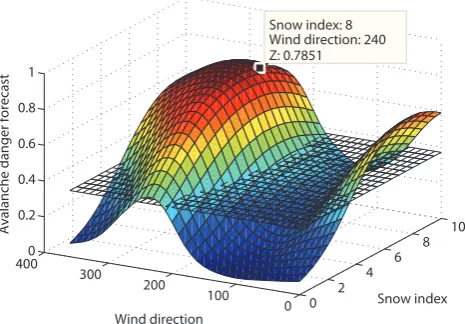
For any particular avalanche path on a given day with associated weather and snowpack conditions, the prediction can be computed by varying the desired parameters in the vicinity of the observed conditions (or most likely conditions from the weather forecast). In particular, model behaviour under the variations of two of the initial avalanching factors is very illustrative. The combinations of every possible values of these 2 variables can take are used to generate the corresponding 39-dimensional input and computing SVM prediction therein. A surface whose height is the SVM decision functionf (x)post-processed into the [0, 1] interval associated with the varying values of the two variables under study is plotted as a result. The choice of the primary variables under consideration can be based on the sensitivity analysis as described above or on forecaster’s experience of what are likely to be the most important factors to explore for a particular case.
As an illustration, the behaviour of the model forecasting avalanche activity for two gullies (see Fig. 1) is examined under changing wind direction and intensity of snowfall (Snow index) since these are indicated to be important features of the avalanche danger in the textual forecast. Figure 6 shows the surface plots of the SVM decision function associated with different weather conditions for the selected gullies.
Figure 6a concerns the behaviour of the model in forecast-ing the avalanche activity in gully A on 9 March 2007, a day for which the current and preceding weather conditions were characterized by easterly/south-easterly winds blowing with snowfalls of high intensity. The conditions on the forecast day are highlighted on the surface with the box visible in the region around a wind direction = 240◦and snow index = 8. On that day an avalanche was observed at this location and the model correctly forecasted the event (hit). The SVM model is consistent in this prediction and provides high danger levels for wide variety of snowfall intensities and wind directions. The danger level decreases for easterly winds (Wind direction∼=90◦), and the indicator of avalanche activity falls below the decision thresholdt (gridded black plane on the figure). This kind of analysis could help to relate model behaviour and the expert’s perception of the influence of individual weather parameters on avalanche conditions.
A. Pozdnoukhov et al.: Spatio-temporal avalanche forecasting with SVM 379
26.12.2006 05.01.2007 15.01.2007 25.01.2007 04.02.2007 14.02.2007 24.02.2007 06.03.2007 16.03.2007
0 0.1 0.2 0.3 0.4 0.5 0.6 0.7 0.8 0.9 Date Avalanche dang er
Profile of avalanche path B Profile of avalanche path A Event at path A Event at path B Event in the region
Fig. 5. Evolution of avalanche danger for gullies A and B during the winter season of 2006/2007.
0 2 4 6 8 10 0 100 200 300 4000 0.2 0.4 0.6 0.8 1 Snow index Snow index: 8
Wind direction: 240 Z: 0.7851 Wind direction Ava lan che da nger forecast
(a) Correctly detected avalanche event on 9 March 2007 at gully A.
0 5 10
0 100 200 300 400 0 0.1 0.2 0.3 0.4 0.5 0.6 0.7 Snow index
Snow Index: 6 Wind direction: 200 Z: 0.3251
Wind direction
Avalanche dange
r fo
recast
(b)
Missed avalanche event on the
3
rdof March
2007 at gully B.
Fig. 6. Behavior of the model dealing with changing Wind direction and Snow index at the selected gullies.
The decision threshold
t
is represented by the gridded black plane at a height of 0.37.
27
26.12.2006 05.01.2007 15.01.2007 25.01.2007 04.02.2007 14.02.2007 24.02.2007 06.03.2007 16.03.2007
0 0.1 0.2 0.3 0.4 0.5 0.6 0.7 0.8 0.9 1 Date Avalanche dang er
Profile of avalanche path B Profile of avalanche path A Event at path A
Event at path B Event in the region
06.01.2007 14.02.2007 03.03.200707.03.200709.03.2007 13.03.2007
Fig. 5. Evolution of avalanche danger for gullies A and B during the winter season of 2006/2007.
0 2 4 6 8 10 0 100 200 300 4000 0.2 0.4 0.6 0.8 1 Snow index Snow index: 8
Wind direction: 240 Z: 0.7851 Wind direction Ava lan che da nger forecast
(a) Correctly detected avalanche event on the
9
thof March 2007 at gully A.
0 5 10
0 100 200 300 400 0 0.1 0.2 0.3 0.4 0.5 0.6 0.7 Snow index
Snow Index: 6 Wind direction: 200 Z: 0.3251
Wind direction
Avalanche dange
r fo
recast
(b) Missed avalanche event on 3March 2007 at gully B.
Fig. 6. Behavior of the model dealing with changing Wind direction and Snow index at the selected gullies.
The decision threshold
t
is represented by the gridded black plane at a height of 0.37.
27
Fig. 6. Behaviour of the model dealing with changing Wind direction and Snow index at the selected gullies. The decision
thresholdt is represented by the gridded black plane at a height
of 0.37.
blowing from the South), Snow index = 6. Figure 6b shows the model predictions according to the variations of the snow intensity and wind direction. While the current prediction falls below the decision threshold, a small variation of wind direction to westerly winds increases the decision function above the threshold plane (when Wind direction∼=270◦). Such an exploration helps in attributing a low level of confidence to the obtained prediction related to possible variations in wind direction.
These examples illustrate how forecasters could graph-ically explore the sensitivity of a particular path to particular variables. However, though potentially a powerful tool, consideration would need to be given to the actual forecasting process. Typically, only a very small part of the forecasters day is spent entering data into a model and exploring results. However, in particular situations, such as
the group discussions carried out by heli-ski guides at daily meetings, such tools might form powerful support services in a suite of knowledge discovery process such as that proposed by McCollister et al. (2003).
5.3 Ensemble of forecasts
Forecasting with an ensemble of models is a conventional approach to describing modelling uncertainties. It is widely accepted in meteorology, hydrology and other fields where uncertainty characterization is considered an essential tool for decision makers in decision making and results dissemination (Gneiting and Raftery, 2005; Anderson and Anderson, 1999; Krzysztofowicz, 2001). A computational approach to explore variability of the model with respect to uncertainty in the input parameters is relatively straightforward. An ensemble of input conditions is sampled from some informative prior distribution (Jaynes, 2003), then the related numerical models (such as those for snowpack spatialisation) are run to generate the secondary input variables, and finally, the ensemble is propagated through the prediction model and the spread of the produced outputs is analysed. The uncertainty with respect to input parameters is irreducible.
The prediction uncertainties concern the inherent proper-ties of the model and assumptions used in modelling process, and the lack or inadequacy of data. This kind of uncertainty estimation in data-driven models is commonly approached in a Bayesian setting (MacKay, 1992). In this work, we consider a computational Monte Carlo ensemble approach to characterize the three sources of uncertainties, one related to the choice of hyper-parameters, one to the choice of samples for the training data set and another related to the input variables.
Our practical implementation of prediction ensemble is composed of the combinations of 5 SVM models (5 different combinations of hyper-parameters), 3 different training subsets and variations in the input parameters (air temperature, wind speed and direction, snowfall intensity), resulting in 540 ensemble members2. An example of the uncertainty characterization for avalanche danger prediction for 15 February 2007 (Fig. 3) with the mean ensemble danger and the related coefficient of variation (COV) is shown in Fig. 7. Here, very low values of danger are excluded to provide a clearer visualisation of the uncertainty in avalanche danger where it is relevant. The excluded values lie mostly on flat valley floors. The most notable feature of the COV is its relatively low values both to windward and leeward of high elevation ridge crests. This suggests that as these locations, irrespective of whether the avalanche danger is high or low, the uncertainty as a result of the ensemble modelling is low. At lower elevations, the COV increases,
2A single prediction computation on the 10 m resolution grid
Fig. 7. Ensemble mean (left) and prediction uncertainty as a coefficient of variation of ensemble predictions (right) on 15 February 2007.
indicating that avalanche danger in these locations is less certain. This accords relatively well with the observations noted in Sect. 4.2 where highest areas of hazard are suggested as being at the highest elevations on north and east facing slopes. The application of such ensemble forecasts is probably more suitable for use by forecasters working over large regions with, perhaps, backgrounds in meteorology and climatology, rather than the forecasters in Lochaber. In the former case, the forecasters are more likely to be primarily office based, and have a good understanding of the potential of ensemble models to interpret uncertainties. By contrast, in the latter case, the primarily field based forecasters may better deal with uncertainty by actually visiting multiple slopes during their daily observations.
6 Conclusions
In this study, avalanche forecasting was considered to be a classification problem, where the aim is to find a decision boundary in the feature space of factors which discriminate “safe” and “dangerous” conditions. Due to the inherent complexity of the phenomenon, noise in data, and dependence on the triggering mechanism, the data entities representing avalanche events and “no events” present highly overlapping sets in any space of conditioning factors decreasing the reliability of Nearest Neighbours methods (McCollister et al., 2003). Moreover, both through theoretical considerations (Beyer et al., 1999) and forecasting practice (McCollister et al., 2003) it has been noted that such methods may be prone to over-fitting when dealing with highly-dimensional data.
Facing a situation in which data collection methods have overtaken our ability to interpret and synthesize data, and the large part of incoming volumes of information remains unexplored, new automated machine learning tools provide a
potential way to extract useful knowledge and dependencies hidden in large volumes of data. Amongst data-driven approaches, expert systems based on simple decision trees and Nearest Neighbours methods are relatively popular with forecasters since they accord well with conventional induc-tive avalanche forecasting processes. However, in machine learning these are considered to be relatively simple pattern classification techniques, and further developments of data-driven predictive tools must provide similar functionality and transparency of interpretation. Sensitivity analysis and uncertainty characterization are essential for bringing these systems into operational use and real-life forecasting practices.
The method explored in this study is a Support Vector Ma-chine, a non-linear classifier which is robust to noise, tolerant to overlapping classes, and showing promising performance in many real life high-dimensional classification problems. The paper provided insights to enhance the interpretability of the developed data-driven prediction system including descriptive historical reference events and a computational analysis of sensitivity and uncertainty. These developments aid in assessing a level of confidence to the obtained avalanche activity predictions related to possible variations in the weather forecasts.
The input conditioning factors used in the forecast were gathered from direct observations of weather and snowpack conditions. To integrate spatial variability into modelling, the main meteorological parameters were spatialised through the use of simple physically-based models. This relatively “naive” modeling of the local meteorology and snowpack could be substituted by a more comprehensive physical models such as, for example, Alpine3D (Lehning et al., 2006). However, the work here demonstrates clearly that SVMs provide a means to generate forecasts which perform well in comparison with more traditional methods such as NN, especially where the data are highly dimensional as is the case in a spatialised forecast. We show a number of ways of presenting the results of SVM based forecasts, ranging from simple maps of danger, through aspect/elevation diagrams to presentation of individual and informative Support Vectors. Since many measurements input to the model are likely to contain uncertainty, we also illustrate how ensemble runs can be produced to illustrate variations in uncertainty for avalanche danger in space.
In conclusion, the main contributions of this paper are: 1. To use a Support Vector Machine to generate avalanche
danger classifications in a spatialised forecast, where physically-based modelling is used to interpolate input data across space.
3. To demonstrate how sensitivity surfaces can help to explore variability of the forecast with respect to individual variables and how ensemble modelling can provide insights into the uncertainties in the modelling of avalanche danger, given knowledge about uncertainty in the input parameters.
In future work we would like to extend this approach to other areas, in particular where more comprehensive avalanche databases would reduce the need to generate virtual events. Furthermore, we see a pressing need for more direct comparison between methods in avalanche forecasting (cf. the Snow Model Intercomparison Project in snowpack modelling; Etchevers et al., 2004) using the same data and success measures. Finally, and most importantly, more dialogue with avalanche forecasters is required to assess the extent to which such approaches could usefully extend the tools that they currently have available to them.
Acknowledgements. This work was partially supported by Swiss
National Science Foundation through the project No.
200020-121835, “GeoKernels: kernel-based methods for geo and
environmental sciences: Phase II”. A. Pozdnoukhov acknowledges the support of Science Foundation Ireland under the National Development Plan, particularly through Stokes Lectureship award
and Strategic Research Cluster grant (07/SRC/I1168). Graham
Moss and the sportscotland Avalanche Information Service are thanked for their assistance in identifying expert features and the provision of data for Lochaber.
Edited by: J. M. Vilaplana
Reviewed by: K. Birkeland and another anonymous referee
References
Anderson, J. and Anderson, S.: A Monte Carlo Implementation of the Nonlinear Filtering Problem to Produce Ensemble Assimilations and Forecasts, Mon. Weather Rev., 2741–2758, 1999.
Barry, R.: Mountain weather and climate, Methuen, London, 1981. Beyer, K., Goldstein, J., Ramakrishnan, R., and Shaft, U.: When Is Nearest Neighbor Meaningful?, Database Theory - ICDT99, 217–235, doi:10.1007/3-540-49257-7 15, 1999.
Bolognesi, R.: Artificial intelligence and local avalanche forecast-ing: the system AVALOG, Proceedings of International Emer-gency Management and Engineering Conference, Arlington, VA, 113–116, 1993.
Brabec, B., Meister, R., St¨ockli, U., Stoffel, A., and Stucki, T.: RAIFoS: Regional Avalanche Information and Forecasting System, Cold Reg. Sci. Technol., 33, 303–311, 2001.
Breiman, L.: Statistical Modeling: The Two Cultures, Stat. Sci., 16, 199–215, doi:10.2307/2676681, available at: http://dx.doi.org/ 10.2307/2676681, 2001.
Buser, O.: Two years experience of operational avalanche
forecasting using nearest neighbors method, Ann. Glaciol., 13, 31–34, 1989.
Doswell, C. A., Davies-Jones, R., and Keller, D. L.: On summary measures of skill in rare event forecasting based on contingency tables, Weather Forecast., 5, 576–585, 1990.
Durand, Y., Giraud, G., Brun, E., Merindol, L., and Martin, E.: A computer-based system simulating snowpack structures as a tool for regional avalanche forecasting, J. Glaciol., 45(151), 469–484, 1999.
Eckert, N., Parent, E., Belanger, L., and Garcia, S.: Hierarchical modelling for spatial analysis of the number of avalanche occurrences at the scale of the township, Cold Reg. Sci. Technol., 50, 97–112, 2007.
Eckert, N., Parent, E., Kies, R., and Baya, H.: A
spatio-temporal modelling framework for assessing the fluctuations of avalanche occurrence resulting from climate change: application to 60 years of data in the northern French Alps, Climatic Change, 101(3–4), 515–553, 2010.
Etchevers, P., Martin, E., Brown, R., Fierz, C., Lejeune, Y., Bazile, E., Boone, A., Dai, Y., Essery, R., Fernandez, A., Gusev, Y., Jordan, R., Koren, V., Kowalczyk, E., Nasonova, O. N., Pyles, R. D., Schlosser, A., Shmakin, A. B., Smirnova, T. G., Strasser, U., Verseghy, D., Yamazaki, T., and Yang, Z.-L.: Validation of the energy budget of an alpine snowpack simulated by several snow models (SnowMIP project), Ann. Glaciol., 38, 150–158, 2004. Gassner, M. and Brabec, B.: Nearest neighbour models for local and
regional avalanche forecasting, Nat. Hazards Earth Syst. Sci., 2, 247–253, doi:10.5194/nhess-2-247-2002, 2002.
Gneiting, T. and Raftery, A. E.: ATMOSPHERIC SCIENCE: Weather Forecasting with Ensemble Methods, Science, 310,
248–249, doi:10.1126/science.1115255, available at: http://
www.sciencemag.org, 2005.
Hart, J. K. and Martinez, K.: Environmental Sensor Networks: A revolution in the earth system science?, Earth-Sci. Rev., 78, 177– 191, 2006.
Hastie, T., Tibshirani, R., and Friedman, J.: The Elements of Statistical Learning, Springer, New York, 2001.
Heierli, J., Purves, R., Felber, A., and Kowalski, J.: Verification of nearest neighbours interpretations in avalanche 300 forecasting, Ann. Glaciol., 38, 84–88, doi:10.3189/172756404781815095, 2004.
Jaynes, E.: Probability Theory: The Logic of Science, Cambridge University Press, Cambridge, 2003.
Keiler, M., Sailer, R., J¨org, P., Weber, C., Fuchs, S., Zischg, A., and Sauermoser, S.: Avalanche risk assessment - a multi-temporal approach, results from Galt¨ur, Austria, Nat. Hazards Earth Syst. Sci., 6, 637–651, doi:10.5194/nhess-6-637-2006, 2006.
Krzysztofowicz, R.: The case for probabilistic forecasting
in hydrology, J. Hydrol., 249, 2–9,
doi:10.1016/S0022-1694(01)00420-6, 2001.
LaChapelle, E.: The fundamental processes in conventional
avalanche forecasting, J. Glaciol., 26(94), 75–84, 1980. Lehning, M., Bartelt, P., Brown, B., Russi, T., St¨ockli, U., and
Zimmerli, M.: SNOWPACK model calculations for avalanche warning based upon a network of weather and snow stations, Cold Reg. Sci. Technol., 30(1–3), 145–157, doi:10.1016/S0165-232X(99)00022-1, 1999.
Lin, Y., Lee, Y., and Wahba, G.: Support Vector Machines for Classification in Nonstandard Situations, Tech. rep., Dept. of Statistics, University of Wisconsin, 2000.
Liston, G. E. and Elder, K.: A Meteorological Distribution
System for High-Resolution Terrestrial Modeling (MicroMet), J. Hydrometeorol., 7, 217–234, 2006.
MacKay, D. J. C.: A Practical Bayesian Framework for
Backpropagation Networks, Neural Comput., 4, 448–
472, doi:10.1162/neco.1992.4.3.448, available at: http:
//www.mitpressjournals.org/doi/abs/10.1162/neco.1992.4.3.448, 1992.
McClung, D. M. and Schaerer, P. A.: The avalanche handbook, The Mountaineers, 1993.
McCollister, C., Birkeland, K., Hansen, K., Aspinall, R., and Comey, R.: Exploring multi-scale spatial patterns in historical avalanche data, Jackson Hole Mountain Resort, Wyoming, Cold Reg. Sci. Technol., 37, 299–313, doi:10.1016/S0165-232X(03)00072-7, 2003.
Platt, J.: Probabilistic outputs for Support Vector Machines and comparisons to regularized likelihood methods, in: Advances in Large Margin Classifiers, MIT Press, 61–74, 1999.
Pozdnoukhov, A., Purves, R. S., and Kanevski, M.: Applying ma-chine learning methods to avalanche forecasting, Ann. Glaciol., 49, 107–113, doi:10.3189/172756408787814870, 2008.
Purves, R. S., Morrison, K. W., Moss, G., and Wright, D. S. B.: Nearest neighbours for avalanche forecasting in Scotland – development, verification and optimisation of a model, Cold Reg. Sci. Technol., 37, 343–355, doi:10.1016/S0165-232X(03)00075-2, 2003.
Schirmer, M., Lehning, M., and Schweizer, J.: Statistical
forecasting of regional avalanche danger using
simulated snow-cover data, J. Glaciology, 55, 761–768,
doi:10.3189/002214309790152429, 2009.
Sch¨olkopf, B. and Smola, A. J.: Learning with Kernels: Support Vector Machines, Regularization, Optimization and Beyond, The MIT Press, 2002.
Schweizer, J. and F¨ohn, P.: Avalanche forecasting – an expert system approach, J. Glaciol., 42(141), 318-332, 1996.
Schweizer, J., Kronholm, K., and Wiesinger, T.: Verification of regional snowpack stability and avalanche danger, Cold Reg. Sci. Technol., 37(3), 277–288, doi:10.1016/S0165-232X(03)00070-3, 2003.
Suter, C. and Harvey, S.: Mobile information systems for avalanche topics, Proceedings of the International Snow Science Workshop, Davos, 391–394, 2009.
Vapnik, V.: Statistical Learning Theory, Wiley, 1998.
Wilks, D.: Statistical Methods in the Atmospheric Sciences,