www.nat-hazards-earth-syst-sci.net/9/779/2009/ © Author(s) 2009. This work is distributed under the Creative Commons Attribution 3.0 License.
and Earth
System Sciences
Large and small scale wave forecast in the Mediterranean Sea
L. Bertotti and L. Cavaleri
ISMAR, Castello 1364/A, 30122 Venice, Italy
Received: 4 September 2008 – Revised: 13 May 2009 – Accepted: 13 May 2009 – Published: 20 May 2009
Abstract. We describe the implementation of an operational high resolution wind and wave forecasting system in the Mediterranean Sea, and then on a limited area centred on the south-east part of Italy, covering parts of the Adriatic and the Ionian seas. We analyse the performance at the two dif-ferent resolutions during the first four months of operation, using the wind and wave data provided by the QuikSCAT scatterometer, and the Jason and Envisat altimeters. Useful accurate forecasts are found up to 72 h range, the maximum operational one. As expected, we find that the limited area models outperform both the wind and wave global or larger scale model results. However, we still find an appreciable un-derestimate by the models for surface wind speed and hence wave height, often concentrated on specific events.
1 Introduction
The operational analysis and forecasting of wind-waves via numerical modelling is a well-established practice, and a substantial volume of literature provides a full description of its present capabilities. See Komen et al. (1994) for a deep look into the physics and numerics of a wave model, Janssen (2007) and The WISE Group (2007) for a review of the present state of the art.
As waves at a certain location depend on the present and past conditions, wind and waves, in a large area surround-ing the spot of interest, a proper estimate at the location of interest needs to consider the whole basin where we are act-ing. Looking at the larger scales, indeed global wave models are operational at several meteo-oceanographic centres pro-viding daily middle-range forecasts, typically up to ten days ahead, for all the global oceans. See, e.g., Janssen (2007)
Correspondence to: L. Bertotti
(luciana.bertotti@ismar.cnr.it)
for the work at the European Centre for Medium-Range Weather Forecasts (ECMWF, Reading, UK) and the website https://www.opr.ncep.noaa.goc for the operational results at the National Centers for Environmental Prediction (NCEP, Camp Spring, Maryland, USA). Bidlot et al. (2002) provide a good review of the performance of the operational systems at some of the main meteo-oceanographic centres.
Unavoidably the use of a global model implies a relatively coarse resolution, generally insufficient when we look at ar-eas characterised by strong spatial gradients, e.g. hurricanes, or close to the coasts where both the orography and the coast-line details introduce in the fields features too small to be seen in the present global model. In these cases a limited area model, working with high resolution and nested in the large scale one, is the commonly accepted solution.
If the basin is enclosed, with no or minor connections to, for instance, an ocean, we can limit our attention to the basin itself, as the outer conditions have no or only minor influence on the ones in the basin. This is the case for the Mediter-ranean Sea, where several models are operational for fore-casts that in general are limited to a few days ahead, see, e.g., http//marine.meteofrance.com,
https://www.previmar.org/previsions/vagues/
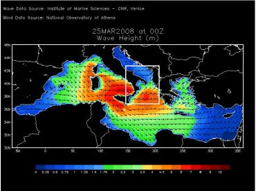
Fig. 1. Output of the father wave model in the Mediterranean Sea. Wave height distribution colour coded according to the scale (metres)
below the figure. Arrows show mean wave direction. The white bordered square shows the area of the nested models.
Fig. 1). The aim was to provide detailed forecasts in the area and particularly on the bordering coasts, especially where the resolutions used for the overall Mediterranean models do not allow sufficient details. The first months of operation have given the chance to explore the capability of the models at their different resolutions. The operational forecasts are available at http://www.riskmed.net/forecastsMain.asp. Our attention has here been focused on part of the Adriatic and the Ionian seas, the latter the large (on a Mediterranean scale) basin to the South of Italy, limited to the West by the Sicily channel (see Figure 1), by Libya to the South, and to the East approximately by the meridian crossing the Peloponnesus. For simplicity throughout the paper we will refer to this area as Ionian. Besides providing more detailed results close to the coasts, we were also keen to explore how much the resolution can affect the general results in the area of interest.
To do this, after providing in Sect. 2 a compact description of the area, in Sect. 3 we describe the models used for the test and their numerical set-up. Sect. 4 is devoted to describe the general meteorology of the period of interest, whose re-sults are presented in Sect. 5. We discuss them and draw our conclusions in the final Sect. 6.
2 The Mediterranean Sea and the sub-area of interest The Mediterranean Sea (see Fig. 1) spans from 6◦W to 36◦E, and from 30◦N to 46◦N. As such, its longitudinal length is close to 3600 km, making it the largest enclosed basin in the world. However, the complicated geometry, characterised by protruding peninsulas, divides the overall basins into a number of smaller sub-basins. Together with the pronounced orography that characterises most of its coasts, this makes the local forecast particularly challenging.
With the exclusion of a few limited areas, namely the Ebro delta in Spain, the Sirte gulf off Tunisia and Libya, the North-ern Adriatic Sea to the East of Italy, and the Nile delta in Egypt, deep water conditions are the rule, with a steeply ris-ing bottom close to the coasts. From the point of view of a wave modeller, with deep water we mean the areas where the sea is deep enough for the waves not to feel the bottom. As an order of magnitude this can be said where the depth is larger than half the maximum wavelength. In the Mediter-ranean this corresponds to 100–150 m.
3 The models
3.1 Meteorological models
Given the need to zoom in on a limited area of the Mediter-ranean Sea, we had to work at two different scales, the first one (termed the “father”) covering the whole basin, providing the boundary conditions for the second one (termed the “son”) focussed on the Ionian Sea.
Mediterranean (father)
The BOLAM model (BOlogna Limited Area Model) is used for operational weather forecasting at the National Observa-tory of Athens (NOA) since 1999. The version of BOLAM used in this study is based on previous versions of the model described in detail by Buzzi et al. (1998) and Buzzi and Fos-chini (2000). A recent evaluation of these operational fore-casts in the Mediterranean region is given in Lagouvardos et al. (2003) with very encouraging results concerning, among other parameters, wind forecasts.
The operational model chain used to provide wind fore-casts to the wave model uses only one grid that consists of 300×270 points with a 0.14 deg horizontal grid interval (∼14 km) centred at 46◦N latitude and 14◦E longitude,
cov-ering a major area of Europe and the whole Mediterranean basin.
In the vertical, 30 levels are used with the model top set at about 10 hPa. The vertical resolution is higher in the surface boundary layer.
The Global Forecasting System (of the National Center for Environmental Prediction, NCEP, USA) provides, among others, gridded analysis fields and 6 hour interval forecasts, at 1.0 degree lat/lon horizontal grid increment. These are used to initialise the model and to nudge the boundaries of the coarse grid during the simulation period. These fields are interpolated on sigma levels from which they are then inter-polated onto the model grid points. The orography fields are derived from a 30 arcsec resolution terrain data file.
The operational runs are initialised every day with the 00:00 UTC GFS analysis. The duration of the simulation is 72 h, providing wind outputs every 3 h, for use by WAM model.
Ionian (son)
High resolution winds, at 4 km intervals, have been provided using the MOLOCH non-hydrostatic atmospheric model (MOLOCH = MOdel LOcal Coordinates Hybrid, in the or-der if its Italian version). See Davolio et al. (2007) for a suitable description. MOLOCH is nested in a version of BO-LAM (16 km resolution) covering large part of the, but not the whole, Mediterranean Sea. BOLAM is nested in the 0.5 degree resolution Global Forecasting System of NCEP. The BOLAM and MOLOCH models are run at the Institute of
Atmospheric Sciences and Climate, ISAC, of the Italian Na-tional Research Council. The 72-h forecast wind fields are available at 3-h intervals starting at 00UTC.
3.2 Wave models
The WAM model (Wave Model; see The WAMDI Group, 1988; Komen et al., 1994; Bidlot et al., 2002; Janssen, 2007 for both fundamentals and applications) has been used for both the scales used in this research. WAM was the first model of the so-called third generation, characterised by being based on pure physics without any a priori assumption on the spectral shape. It considers all the basic processes, namely in deep water generation by wind, nonlinear wave-wave interactions, and white-capping, that control the evolution of a wave field. It is amply described in the literature, both as fundamentals and applications.
Mediterranean (father)
Two grids have been tested, respectively at 1/8 and 1/4 de-gree resolution. As it will soon be explained, for the oper-ational applications the final choice was 1/4 degree. Taking the western border of the grid at 6◦W corresponds to con-sidering the Gibraltar strait to be closed. This may affect the estimated wave conditions in the nearby area, but certainly not so in the limited area marked in Fig. 1. The spectra have been defined on 30 frequencies, in geometric (1.1) progres-sion from 0.05 to 0.8 Hz, and 24 uniformly spaced directions starting at 7.5 degrees with respect to North. The integration time step was 300 and 900 s respectively for the 1/8 and 1/4 degree resolution.
The wind input information, at three hour intervals, has been provided by the Mediterranean BOLAM described above, then bi-linearly interpolated on the wave grid. Each daily forecast covers the following 72 h. The 24 h forecast of the previous day (2-D spectra on the whole grid) is taken as initial conditions for the new forecast. The output wave conditions are available at three hour intervals, at synoptic times (00:00, 03:00, 06:00, . . . UTC). For the following nested run the directional spectra are saved at each time step at all the border points of the nested area (see Fig. 1). Ionian (son)
resolution and at each time step, are given by a space and time interpolation from the 2-D spectra (see above) stored during the integration of the father model.
Taking as reference the product “number of grid points times the number of integration time steps per real hour”, we find for the three considered implementations:
Mediterranean 1/8 16 172×12∼194 K Mediterraenan 1/4 3758×4∼15 K Ionian 1/16 5750×20∼115K
These figures are proportional to the computer time re-quired for the different implementations. For operational ac-tivity we try to limit the necessary computer time, provided the quality of the results remains the same. Therefore two series of runs have been done where the boundary conditions for the son were provided respectively by the 1/8 and 1/4 father versions. The comparison between the two sets of re-sults showed that the average differences were irrelevant, at most of the order of a few centimetres. Apart from the irrel-evance of these quantities for practical applications, they are well below the expected errors of the combined meteo+wave models (see The WISE Group., 2007, for a full discussion on the subject). Therefore for operational applications we resorted to the use of the 1/4 father version.
4 The climatology of the area
To judge the performance of the operational system we use the results from the first four months of activity, i.e. the pe-riod January–April 2008. During these months the climate of the area has been sufficiently representative of the long term one during the winter and spring months. The strongest storms are associated to the bursts of mistral in the north-western part of the basin (with mistral we mean the strong north-westerly wind blowing down in the gulf of Lion from the Carcassone pass). Depending on the trajectory of the front or possibly of the low that comes with it, we find in the Ionian Sea either a north-westerly wind blowing off the Ital-ian coast, or, more frequently, first a frontal south-westerly wind turning to north-west after the passage of the front. Such an event happened on 25 March and it is shown in Fig. 1.
Another source of stormy conditions is from the East, by the winds turning to the right, passing between Greece and Crete, after descending along the Aegean Sea (25–26 Jan-uary, 9–10 February). Occasional light storms are from the South, all the way from the African coast. Some northerly storms appear when a high pressure zone sets on Europe, ad-vecting, possibly with the help of a low pressure to the East, cold Siberian air all over the Adriatic Sea (bora) that, if ex-tended enough, can reach the Ionian Sea (17–18 February). Apart from the storms, conditions are mild, with the waves reacting to more or less local winds of variable direction.
On the whole the events of the four month period were suf-ficiently representative of the conditions in the area to con-sider the derived statistics of the performance of the mete-orological and wave models as sufficiently representative of their long term behaviour.
5 Results
In the present paper our aim is to compare and analyse the performance of the meteorological and wave models at the Mediterranean and Ionian scales during their first four months of operational use. To be fully representative we focus our analysis to the area marked in Fig. 1, where the MOLOCH and wave son models have been run. We have analysed the performance of the models separately for each 24 h forecast (0–24, 24–48, 48–72), and we will go into de-tails for the 0–24 h range.
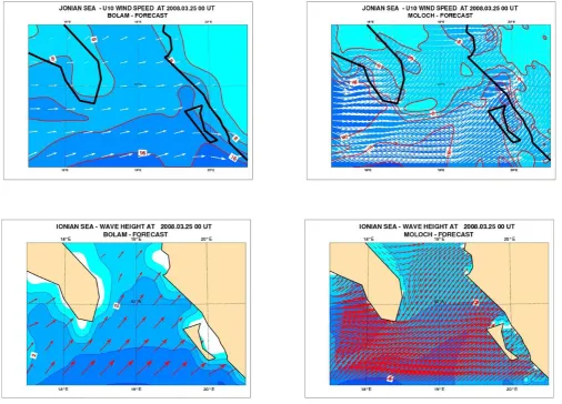
A first comparison is done in Fig. 2, where we zoom in on a small part of the Ionian and plot the wind (upper pan-els) and wave (lower panpan-els) fields with their full resolution. The “father” results are on the left, the ‘son’ ones on the right. The compromise between the needs to show a not too small area and at the same time all the values (arrows) of the high resolution model makes the right plots rather dense. Nevertheless it is possible to pinpoint significant differences between the results of the two resolutions. This is true es-pecially close to the coast, where the 7×5 km resolution of the wave son is able to show very realistic variations along the coastline, something clearly not possible with the father (28×20 km). Note in particular in the nested model the ar-ticulated wave field around the Italian peninsula. Note also the capability of the son models to represent the Kerkyra is-land, just off the Greek coast, behind which is the port of Igoumenitza, that was one of the targets of the project lead-ing to this work.
Apart from the details of the coastline, the resolution be-comes essential in areas characterised by strong spatial gra-dients. Here the rapid variations of the wind direction lead to cross-sea conditions, i.e. to contemporary wave systems at a certain location moving in very different directions. This is especially true when the front is moving quickly, that is typical of mistral. Cross-seas, more so if in heavy sea areas, are among the worst conditions to be faced by sailors. The smoothing of the fields associated to a relatively coarse reso-lution tends to widen the transition area, hence to smooth the field, possibly misinterpreting the worst conditions, a feature that is not easily recognised looking only at the significant wave height Hs fields. In this respect please note that plot-ting the significant wave heights and mean wave directions hides the actual energy distribution. The full information is available only analysing the full 2-D spectra.
Fig. 2. Upper panels: wind fields; lower panels: wave fields. Left: father model; right: son model. The view is zoomed in on the central-right
part of the nested area in Fig. 1.
RON (De Boni et al., 1993) has ceased working since a few months ago. Hence we rely on satellite data. In particu-lar we retrieved QuikSCAT scatterometer data and altimeter data from Jason and Envisat satellites. The used scatterom-eter data are at 50 km intervals on a 1800 wide swath. They are not available close to the coasts. Nevertheless they pro-vide a solid judgement about the quality of the model wind fields. For altimeters, the data are available at 7 km inter-vals along the ground track of the satellite. The measurement area at each altimeter pulse has a diameter of a few kilome-tres, the actual size depending on the sea state. When the satellite is passing from land to sea, no measurements are available till 20 km or more off the coast (the situation is bet-ter with the latest altimebet-ters, e.g. Jason-2). When the flight is toward the land, the data are available at shorter distances from the coast. There is an ample literature on both these in-struments, see, among others, Hoffman and Leidner (2005), Chelton et al. (2004), Chelton and Freilich (2005), Dobson et al. 1987), Monaldo (1988), Witter and Chelton (1991), Gourrion et al. (2002), Gommerginger et al., (2002).
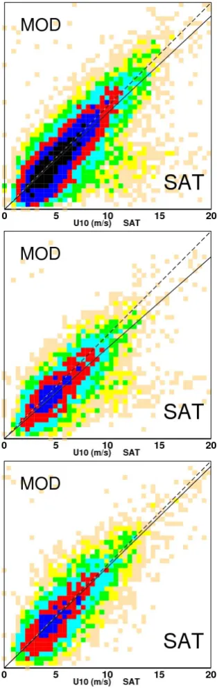
Table 1. Best-fit slope and scatter index of the model wind speeds
vs scatterometer measured data. Two different models and two dif-ferent areas are considered.
best-fit slope scatter index
BOLAM Mediterranean 0.94 0.35
BOLAM Ionian 0.87 0.33
MOLOCH Ionian 0.98 0.31
Fig. 3. (a) Scatter diagram between BOLAM model wind
speeds vs. scatterometer measured data. The area is the whole Mediterranean Sea. (b) As Fig. 3a), but for the Ionian Sea. (c) As Fig. 3a, but for the MOLOCH model and the Ionian Sea.
We begin discussing the general wind fields. Figure 3 provides a direct comparison (scatter diagrams) between the scatterometer and the model wind speeds. Figure 3a refers to the performance of BOLAM in the whole Mediterranean Sea, Fig. 3b to BOLAM in the Ionian Sea (i.e. the area
marked in Fig. 1), Fig. 3c to MOLOCH in the Ionian. Each plots shows the best-fit line (highlighting the general per-formance of the model) and the scatter of the data around it, summarised in the scatter index SI, defined as the ratio between r.m.s. model error and the mean measured value. These results for three plots are given in Table 1. In the fig-ure the different colour pixels provide an information about the number of data in each pixel. The colour scale is given in Table 2.
From Fig. 3a and Table 1 it is clear that BOLAM performs sufficiently well in the overall Mediterranean, although the scatter is quite large (SI=0.35). There a 6% average under-estimate, that could be partially due to the bunch of data in the lower-right part of the figure. For our present purposes it is interesting to look at the BOLAM performance in the Ionian. Here the scatter is slightly reduced (SI=0.33), but the average underestimate is increased to 13%. Note the similar bunch of data (large satellite values, low model ones) that, if associated to a specific event, may affect the best-fit slope to a larger extent because of the lower overall number of data considered. The situation is much improved when we move to the nested model, MOLOCH (Fig. 3c), where there is an almost negligible underestimate (2%) and a further reduced scatter (SI=0.31). Note that the bunch of data in the lower-right part of the figure has disappeared.
A different format is used for the presentation of the model vs altimeter intercomparison results. These are reported in Fig. 4, a) for the whole Mediterranean using BOLAM winds, b) the same, but focussed on the Ionian (see Fig. 1), c) for the MOLOCH winds, again in the Ionian. Each plot conveys various information. The continuous blue and red lines (re-spectively for wave and wind) show the differences “model-altimeter” for the significant wave height Hs (m) and wind speed U (ten metre wind speed, m/sec) as a function of the measured quantities. Note that, to use a single diagram, on the horizontal scale we have plotted U/2 and 2*Hs. The ver-tical axis (differences) has the same scale for both the quan-tities (m, m/sec). The dash lines show the corresponding per-centual differences, with 1. corresponding to 100%. The little squares indicate the number N of available data (shown as log10N) in each horizontal range section. For N>1000 the squares are out of the used axis range in the Mediterranean (Fig. 4a), showing the relevance of the low wind speeds and wave heights in this basin. For wind speeds this was already evident from Figure 3a. Note the distribution of black pixels, the ones (see Table 2) with the largest number of data.
Table 2. Number of data in each pixel of Fig. 3 according to the
colour.
colour beige yellow green light blue red blue black
number 1–3 3–5 5–9 9–1 18–36 36–73 73–150 of data
Fig. 4. (a) Bias (vertical scale) of the model vs. Envisat
altime-ter wind speeds U and significant wave heights Hs. The continu-ous lines show the absolute biases, the dash onse the percent error (model – altimeter), for different U and Hs ranges. Note the dif-ferent scaling for these two quantities (horizontal axis). The little squares show the number of data in each range. Log10 scale has been used. The area considered is the whole Mediterranean Sea. The atmospheric model is BOLAM. (b) as Fig. 4a, but for the Io-nian Sea. (c) As Fig. 4a, but for the MOLOCH model and the IoIo-nian Sea.
the results for the very low value range. At the opposite side it is worthwhile to point out that, due to the lower number of data, the results for the high value range are less reliable and should be handled with care.
After considering the results for the whole Mediterranean Sea, it is instructive to look at those for the Ionian (Figure 4b), when using the same wind source. The immediately ev-ident characteristic is the strong underestimate of the wind speed in the range between 6 and 12 m/sec. While the pre-cise values are uncertain (note the limited number of data), the overall significance is clear. Somehow the model misses a significant event. There is an expected corresponding in-crease of the percent wind error and also, albeit much more limited, of the wave height error (just by chance, the use of different scales for U and Hs seems to bring together in the plot the two corresponding underestimates). In this respect we must remember that the waves represent an integrated ef-fect, in space and time, of the driving winds, hence they do not react emphatically to a “local”, albeit large, wind under-estimate. Therefore, although wind and wave were measured at the same time and position, and although the wind speed was locally underestimated by the models (see the maximum wind bias in Fig. 3), the wave height biases do not show such a peak.
As the data used for Fig. 4b are a sub-section of the ones used for Fig 4a, the just discussed miss should appear also in the Mediterranean plot, although much reduced because mixed with a much larger amount of data. Indeed this is the case, as we can see looking again at Fig. 4a, where the local mimima around U/2=2*Hs=8 do correspond to the drastic underestimate in Fig. 4b.
Moving finally to the nested MOLOCH model and the de-rived wave data, in principle one could think that the substan-tial error present in the coarser model should disappear or, at least, decrease substantially. However, at a further thought, this turns out not to be the case. The nested model carves out details, and eventually different evolutions, of the fields pro-vided by the father model. In so doing, one would expect an improvement (see, e.g., the spectacular results by Cardone et al., 1996). However, this is true when the event is limited to the considered, nested scale. If, as we suspect to be the case, the event has a larger scale, then the son model is forced to act on initial and boundary “wrong” information, which un-avoidably leads to similar wrong results. This could well have been the case for the considered event.
It is highly tempting to relate these underestimates with the bunch of data (lower-right corner) repetitively mentioned while discussing the scatterometer data (see Fig. 3a and b). While we have identified one possible “culprit” storm (23 January 2008), a deeper analysis of these events will be the subject of a further devoted study.
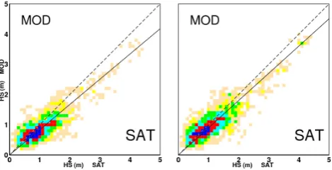
their performance. On one hand the already quoted exten-sive literature existing on the subject has repetitively pointed out the difficulty for the altimeter to measure very low wind speeds. This becomes even more true (see in particular Gom-merginger et al., 2002) in the presence of swell, that modu-lates and tilts the tiny wavelets created by the weak wind. As far as the models are concerned, quite often in the open sea the required information, i.e. a sufficiently dense network of measured data, is missing, and somehow the models are not able to follow up the situation. It is interesting that there is no corresponding bias of the wave heights. However, this is not highly significant because on one hand, as repetitively pointed out, waves are not strictly associated to the local wind conditions. On the other one we are talking about a range that is not significant for practical applications, either for atmosphere-ocean exchanges (matter, gas, energy, etc), or for engineeristic purposes (no wave generation). While a deeper analysis of the matter is out of the scope of the present analysis, we simply point out that having similar results for both the BOLAM and MOLOCH models tends to suggest that indeed the problem is mainly associated to the altimeter. We conclude our analysis with the scatter diagrams of the model vs altimeter significant wave heights for the nested area. They are shown in Fig. 5, left for the father, right for the son. The two best-fit slopes and scatter indices are re-spectively 0.84 and 0.29, 0.90 and 0.30. The underestimates reflects what seen in Fig. 4b and c. There is a clear improve-ment passing from the father to the son model. The scatter is still large, but lower than for wind speed, reflecting the char-acteristics of a wave field, which intrinsically tends to smooth the variability of the model around the measured data. It is interesting to argue where this comes from. Partly this may come from the higher resolution wave model used for the son run (see Sect. 3). As we have discussed, this can be in the front areas, more in general in zones characterised by strong gradients, or in the coastal areas. Both these facts have prob-ably a limited influence on the results shown in Fig. 5, on one hand because fronts are not very common, on the other one because the percentage of altimeter data close to the coast-lines is limited (see above). We believe that most of the im-provement is due to the use of improved, nested wind fields, as on the other hand we have seen in Fig. 3b and c.
All the above results hold for forecasts up to 24 h. How-ever, the statistics have been evaluated also for the following 24–48 and 48–72 h ranges. The results are very similar, par-ticularly for the best-fit slopes and the biases as functions of the measured variables. The basic differences are in the value of the scatter indices, growing with the extent of the forecast range.
6 Discussion
The results presented in the previous section deserve some further discussion. Although partly justified by the different
Fig. 5. Scatter diagrams of father (left) and son (right) wave model
results with respect to the values measured by the Jason altimeter. In each pixel the colour shows approximately the number of cases considered in that range. From high to low numbers in geometric scale: blue, red, light blue, green, and yellow.
levels of performances in the different ranges, the values of the best-fit lines obtained for wind speed and wave height are not fully consistent with each other. There are two possi-ble explanations for this: a) a poor performance, basically a substantial underestimate, by the WAM wave model, or b) a poor performance of the altimeter, with either an underesti-mate of the measured wind speeds, or an overestiunderesti-mate of the measured Hs. We tend to exclude the first possibility, cer-tainly so in the range of the underestimates seen in Figs. 4 and 5. WAM is a very well tested and verified machine, as repetitively pointed out in the literature. Indeed, see in par-ticular Janssen (2007), the performance of a third-generation wave model, as WAM, is considered as the best way to check the quality of the driving wind fields. Therefore we focus on the wind and waves measured by the altimeters. Here we move to a less safe ground, especially for the wind speed. Indeed, many previous verifications, see among others The Medatlas Group (2004), Ardhuin et al. (2007), and Bertotti and Cavaleri (2008), lead to the conclusion that, while the Hs altimeter measurements, when properly corrected, are highly reliable, the U data in the Mediterranean are generally under-estimated. The specification for the area stems from the fact that (see Gommerginger et al., 2002) the wave conditions do affect the altimeter wind speed measurements, and the gen-eral wave conditions in an inner sea, as our present area of interest, are different from the ones in the oceans where the satellite instruments have generally been calibrated. In any case the quoted previous results are consistent with our find-ings, with a U altimeter underestimate that, from the corre-sponding Hs data, we judge around 10%.
percents, than the ones of the fathers. Ironically, this repre-sent the capability of the son models to go into higher details of the fields. However, the capability of reproducing real-istic details does not imply these details are correct. Given a certain level of scatter between the actual data and a rel-atively smooth (lower resolution) field, the introduction of higher resolution details, physically consistent but not neces-sarily coincident with the real ones, leads unavoidably to a larger scatter (this is usually referred to as double penalty). Of course, for the just mentioned reason, this is partly filtered out in the wave results.
It is instructive to compare the performance of the father and son models considered here with those of global models, e.g. of ECMWF. Their global statistics show best-fit slopes for wind and wave very close to unity, with scatter indices close to 10%. However, this is true for the open oceans. In the enclosed seas, and in particular in the Mediterranean Sea (see Cavaleri and Bertotti, 2006, and The Medatlas Group, 2004), the quality of the performance drops substantially. It improves with increasing resolution, and indeed the perfor-mance of the son models we have considered outperforms the ones of ECMWF. However, clearly this is still not enough to reduce the biases to the level of the present performance in the open oceans. Along the same line of thinking we argue that the reason for the improved quality of the MOLOCH wind fields with respect to the BOLAM ones is their higher resolution plus the corresponding improved physics of the model. The resolution is particularly relevant because the area is under the “shadow” of the Italian peninsula. While remarkable storms are possible from all the directions, the dominant wind pattern brings the substantial events from the north-west direction, i.e. from the Italian and Sicily coast-lines and orography. Especially in the peninsula the relevant orographic features do affect the wind in their lee side, some-thing clearly dealt better the higher the model resolution.
The persistent quality of the performance while consider-ing different forecast ranges show that the models, implicitly the father and the global ones, correctly forecast the wind, hence the wave, conditions up to at least a three day distance. Rather than on the intensity of the possible storms, the un-avoidable, although limited, errors concern small deviations in space and time. In practice a storm may follow a slightly different path (error in space) or move faster or more slowly than anticipated (error in time). If the strength of the event is correctly anticipated, these errors do not imply an apprecia-ble variation of the bias or the best-fit slope, but a substantial increase of the scatter index. Unluckily, from this point of view the use of a higher resolution, nested model does not improve much the situation. A nested model behaves accord-ing to the information it starts from (the father model) and the subsequent boundary conditions along the forecast range. If a time or space error is present in the father model, this will unavoidably be reflected, possibly amplified, in the son model. Using a rather pessimistic expression, nested mod-els are capable of exceptional performances, but also of very
well carved mistakes. Nesting cannot be taken as the “every-thing solving solution”. They simply focus on the details of a given area, and, fully relying on their father, they do it cor-rectly provided they receive the correct information. Their use must not slow down the effort to improve the global or large scale models, the source of the basic information.
Acknowledgements. The present work has been carried within the project “Weather Risk Reduction in the Central and Eastern Mediterranean – RISKMED”, as part of the EU Community Initiative Programme INTERREG IIIB – ARCHIMED.
Edited by: A. Mugnai
Reviewed by: J. Wolf and one anonymous referee
References
Ardhuin, F.,Bertotti, L., Bidlot, J.-R.,Cavaleri, L.,Filipetto, V.,Lefevre, J.-M., and Wittmann, P.: Comparison of wind and wave measurements and models in the Western Mediterranean Sea, Ocean Eng., 34(3–4), 526–541, 2007.
Bertotti, L. and Cavaleri, L.: Analysis of the Voyager storm, Ocean Eng., 35(1), 1–5, 2008.
Bidlot, J.-R., Holmes, D. H., Wittmann, P. A., Lalbeharry, R., and Chen, H.S.: Intercomparison of the performance of operation ocean wave forecasting systems with buoy data, Weather Fore-cast., 17, 287–310, 2002.
Buzzi A., Tartaglione, N., and Malguzzi, P.: Numerical simulations of the 1994 Piedmont flood: role of orography and moist pro-cesses. Mon. Weather Rev., 126, 2369–2383, 1998.
Buzzi, A. and Foschini, L.: Mesoscale meteorological features as-sociated with heavy precipitation in the southern Alpine region, Meteorol. Atmos. Phys., 72, 131–146, 2000.
Cardone, V. J., Jensen, R. H., Resio, D. T., Swail, V. R., and Cox, A.T.: Evaluation of contemporary ocean wave models in rare extreme events: the “Halloween storm” of October 1991 and the “Storm of the century” of March 1993, J. Atmos. Ocean Tech., 13, 198–230, 1996.
Cavaleri, L. and Bertotti, L.: The improvements of modelled wind and wave fields with increasing resolution, Ocean Eng., 33(5–6), 553–565, 2006.
Chelton, D. B. and Freilich, M. H.: Scatterometer-based assessment of 10-m wind analyses from the operational ECMWF and NCEP numerical weather prediction models, Mon. Weather Rev., 133, 409–429, 2005.
Chelton, D. B., Schlax, M. G., Freilich, M. H., Milliff, R. F., and Vandemark, D. C.: Satellite measurements reveal persis-tent small-scale features in ocean winds, Science, 303, 978–983, 2004.
Davolio, S., Buzzi, A., and Malguzzi, P.: High resolution simulation of an intense convective precipitation event, Meteorol. Atmos. Phys., 95, 139–154, 2007.
De Boni, M., Cavaleri, L., and Rusconi, A.: The Italian wave mea-surement network, Proc. 23rd Int. Conf. on Coastal Engineering, Venice, Italy, Amer. Soc. Civil Eng., 1840–1850, 1993. Dobson, E., Monaldo, F., and Goldhirsh, J.: Validation of Geosat
Gommenginger, C. P., Srokosz, M. A., Challenor, P. G., and Cotton, P. D.: Development and validation of altimeter wind speed algo-rithms using an extended collocated buoy-TOPEX dataset, IEEE T. Geosci. Res. Sens., 40(2), 251–260, 2002.
Gourrion, J., Vandemark, D., Bailey, S., Chapron, B., Gommergin-ger, G. P., Challenor,P. G., and Srokosz, M. A.: A two-parameter wind speed algorithm for Ku-band altimeters, J. Atmos. Ocean. Tech., 19, 2030–2048, 2002.
Hoffman, R. N. and Leidner, S. M.: An introduction to the near-real-time QuikSCAT data, Weather Forecast., 20, 476–493, 2005.
Komen, G. J., Cavaleri, L., Donelan, M., Hasselmann, K., Hassel-mann, S., and Janssen, P. A. E. M.: Dynamics and Modelling of Ocean Waves, Cambridge University Press, 532 pp., 1994. Janssen, P. A. E. M.: Progress in ocean wave forecasting, J. Comp.
Sci., 227(7), 3572–3594, 2007.
Lagouvardos, K., Kotroni, V., Koussis, A., Feidas, C., Buzzi, A., and Malguzzi, P.: The meteorological model BOLAM at the National Observatory of Athens: assessment of two-year oper-ational use, J. Appl. Meteor., 42, 1667–1678. 2003.
The Medatlas Group: Wind and wave atlas of the Mediterranean Sea, Western European Union, WEAO Research Cell, 419 pp., 2004.
Monaldo, F.: Expected differences between buoy and radar altime-ter estimates of wind speed and significant wave height and their implications on buoy-altimeter comparisons, J. Geophys. Res., 93(C3), 2285–2302, 1988.
The WAMDI Group: The WAM model – a third generation ocean wave prediction model, J. Phys. Oceanogr., 18, 1775–1810, 1988.
The WISE Group – Cavaleri, L., Alves, J.-H. G. M., Ardhuin, F., Babanin, A., Banner, M., Belibassakis, K., Benoit, M., Donelan, M., Groeweg, J., Herbers, T. H. C., Hwang, P., Janssen, P. A. E. M., Janssen, T., Lavrenov, I. V., Magne, R., Monbaliu, J., Ono-rato, M., Polnikov, V., Resio, D., Rogers, W. E., Sheremet, A., McKee Smith, J., Tolman, H. L., van Vledder, G., Wolf, J., and Young, I.: Wave modelling – the state of the art, Prog. Ocean., 75(4), 603–674, 2007.