www.nat-hazards-earth-syst-sci.net/11/1189/2011/ doi:10.5194/nhess-11-1189-2011
© Author(s) 2011. CC Attribution 3.0 License.
and Earth
System Sciences
Stochastic index model for intermittent regimes: from preliminary
analysis to regionalisation
M. Rianna, F. Russo, and F. Napolitano
Dipartimento di Ingegneria Civile, Edile e Ambientale, Sapienza Universit`a di Roma, Via Eudossiana 18, 00184 Roma, Italy Received: 19 June 2010 – Revised: 24 December 2010 – Accepted: 18 February 2011 – Published: 27 April 2011
Abstract. In small and medium-sized basins or in rivers characterized by intermittent discharges, with low or negligi-ble/null observed values for long periods of the year, the cor-rect representation of the discharge regime is important for issues related to water management and to define the amount and quality of water available for irrigation, domestic and recreational uses. In these cases, only one index as a statis-tical metric is often not enough; it is thus necessary to intro-duce Flow Duration Curves (FDC).
The aim of this study is therefore to combine a stochastic index flow model capable of reproducing the FDC record pe-riod of a river, regardless of the persistence and seasonality of the series, with the theory of total probability in order to calculate how often a river is dry.
The paper draws from preliminary analyses, including a study to estimate the correlation between discharge indica-tors Q95, Q50 and Q1 (discharges exceeding 95%, 50% or
1% of the time, respectively) and some fundamental char-acteristics of the basin, as well as to identify homogeneous regions in the target area through the study of several geo-morphological features and climatic conditions. The stochas-tic model was then applied in one of the homogeneous re-gions that includes intermittent rivers.
Finally, the model was regionalized by means of regres-sion analysis in order to calculate the FDC for ungauged basins; the reliability of this method was tested using jack-knife validation.
1 Introduction
An accurate representation of a river regime is essential to several engineering applications, such as the analysis of hydroelectric feasibility, reservoir and lake sedimentation,
Correspondence to: M. Rianna
water resources management and environmental planning. An important environmental problem related to this issue is wastewater discharge into rivers: in fact, legislation has restricted discharge into rivers characterized by no flow for long periods.
Flow Duration Curves (FDC), which represent the per-centage of time during which the discharge of a river is ex-ceeded, can be used as a tool to accurately represent the streamflow frequency regime and can be applied to all these hydrological applications. The FDC can be easily calculated as the complement of the cumulative distribution function (cdf) from a gauged river; this information is also essential for ungauged basins.
FDC characteristics were synthesised by Searcy (1959). Later, Smakhtin (2001) revised the argument on low flows in hydrology, outlining the use of flow duration curves that had been used up to then. FDC have been calculated in ungauged basins in several studies (Quimpo et al., 1983; Mimikou and Kaemaki, 1985; Claps and Fiorentino, 1997; Smakhtin et al., 1997; Ganora et al., 2009); additional stud-ies have provided analysis of the uncertainty of FDC (Yu et al., 2002) and the development of a stochastic model for calculating FDC (LeBoutillier and Waylen, 1993; Cigizoglu and Bayazit, 2000). Vogel and Fennessey (1994) introduced Annually-Based Flow Duration Curves (AFDC), which are useful for making probabilistic considerations of the dis-charge of dry, wet and average years and for calculating the inter-annual variability associated with AFDC. Castellarin et al. (2004) introduced a similar approach to that of the dis-charge index to model the relationship between FDC and AFDC in daily discharges. This method can reproduce FDC and also mean, median and variance of AFDC without as-sumptions based on the seasonal and persistence structure of daily discharges.
1190 M. Rianna et al.: Stochastic index model for intermittent regimes base flow, or their base flow is restricted to only the wet
pe-riods of the year, while for the rest of the year there is no flow.
The presence of zeros in a discharge time series can be real or can occur when the discharge is beneath a threshold and the instruments cannot take any measurements, as in the case of censored data (Durrans et al., 1999). Several studies have focused on various methods to work with zero data in fre-quency analysis (e.g. Jennings and Benson, 1969; Kilmartin and Peterson, 1972; Haan, 1977; Wang and Singh, 1995), while others have concentrated more on techniques for work-ing with censored data (e.g. Kroll and Stedwork-inger, 1996; Tate and Freeman, 2000).
The occurrence of zero events can be expressed in prob-ability theory by substituting a non-zero probprob-ability mass with a zero value. This creates a discontinuity in the density function from which the hydrological series is obtained, with discontinuity in the zero value. However, this solution can create problems with the assumption of continuity made in frequency analysis. Jennings and Benson (1969) highlighted the potential problems encountered when a continuous dis-tribution is fitted with data including zero values.
The literature presents three methodologies for approach-ing zero data, summarized in Haan (1977):
– The first is to add a small constant to all observations, such as 1% of the mean magnitude, and fit a continuous distribution such as the Log-Pearson type III distribu-tion onto the data (Subcommittee on Hydrology, 1966). This approach can move the discontinuity represented by the zero state but does not solve the problem created by the discontinuity.
– The second ignores the zero values and considers only the non-zero values and then corrects the results for the entire period recorded. Haan (1977) and Wang and Singh (1995) showed that this method is biased, since it ignores all zero values in the data.
– The third is based on the theorem of total probability (Jennings and Benson, 1969).
Woo and Wu (1989) and Wang and Singh (1995) developed empirical three-parameter models for the frequency analysis of hydrologic data containing zero values starting from the theorem of total probability. On the other hand, Strupczewski et al. (2003) proposed a different method based on the hy-pothesis that the unit impulse response of a linearized Kine-matic Diffusion (KD) model is a probability distribution suit-able for frequency analysis of hydrologic samples with zero values.
The principal aim of this paper is to create a model to cal-culate FDC for daily streamflows that also works in basins with intermittent flow in dry climates. In order to reach this objective, the model combines the stochastic index flow
model (Castellarin et al., 2004) with the theory of total prob-ability. The stochastic index flow model allows for the com-putation of a river’s FDC without regard to the persistence and seasonality of the series and enables the calculation of conditional distributionF (y|Y >0), while the theory of total probability allows an evaluation of the percentage of time the river is dry. A procedure of regionalisation of the model is also applied based on the definition of homogeneous regions in the target area and allows for the definition of equations that permit the transfer of the model to ungauged basins.
This paper is organized as follows:
1. Definition of the modified stochastic index flow model. 2. Presentation of a case study and the regionalisation
method.
3. Application of the methodology and discussion of the results.
4. Summary and conclusions.
2 The modified stochastic index flow model 2.1 Flow duration curves
The FDC provide information about the percentage of time a particular streamflow was exceeded over a given historical period. For a daily flows series, the FDC can be seen as the complement of the cumulative distribution function of daily streamflows based on the complete recording of flows.
A nonparametric approach to construct the FDC can there-fore be used (Vogel and Fennessey, 1994):
– By re-assembling the observed streamflows in ascend-ing order.
– By plotting each observation versus its corresponding duration or exceedance probability. Duration is often expressed as a percentage and coincides with an esti-mate of the exceedance probability,ei, of thei-th
ob-servation in the ordered sample. ei can be estimated
using an empirical distribution such as the Weibull plot-ting position. DurationDi is thus
Di=100(ei)=100·
1− i
n+1
,
for i=1,2,3,...,n (1)
wherenis the length of the sample.
It is possible to build FDC with different time resolu-tions of the discharges, but daily FDC offer the most detailed means of examining the duration characteristics of a flow.
2.2 Standard stochastic index flow model of FDC The approach used here assumes that daily streamflowXcan be found by multiplying an index flow equal to annual flow AF by a dimensionless daily streamflowX0,
X=AF·X0 (2)
The climatic conditions and annual precipitation given for a basin affect AF. The probability density function,fX0of stan-dardized flows is correlated with the geomorphologic charac-teristics of the basin.
Using this formulation, it is possible to calculate FDC for the complete recording period of flows as the complement of the cumulative distribution function (cdf) ofX,FXgiven by:
Fx(x)=Pr{X≤x} = x
Z
xl
fX(u)du=PrAF·X0≤x
= Z
X0
x/z
Z
afl
fAF,X0(ν,z)dvdz (3)
Y = domain of a given random variableY;fX= pdf ofX;
fAF,X0= joint probability distribution of AF andX0; xl and afl= lower bounds ofX0 andAF, respectively.
If it is assumed that AF and X0 are independent, then fAF,X0 equals the product of the two marginal distributions, and it is possible to write:
FX(x)=
Z
X0 fX0(z)
x/z
Z
afl
fAF(ν)dνdz= Z
X0
fX0(z)FAF(x/z)dz
(4) whereFAF= cdf of AF;fX0= pdf ofX0.
The FDC can be estimated by plotting the variable X against the duration, equal to 100(1−FX) (Castellarin et al.,
2004).
2.3 Stochastic index flow model in the presence of zero data
The problem of the presence of zero data can be solved us-ing the theorem of total probability, which is used to deter-mine the probability of occurrence of a non-zero event, given that a zero event has already occurred (Jennings and Benson, 1969).
The theorem is given by:
Pr(X > x)=Pr(X > x|X=0)Pr(X=0)
+Pr(X > x|X6=0)Pr(X6=0) (5) Thus, given that Pr(X > x|X=0) is zero, and writing this relationship in the form of cumulative probability distribu-tions, it is possible to obtain Pr(X≤x):
Pr(X≤x)=pdry+pnzPr(X≤x|X6=0) (6)
wherepnz= the percentage of time that the river is flowing
(i.e. Pr(X6=0)).pnzcan be estimated using the plotting
po-sition formulation;pdry= the percentage of time the river is
dry, equal to 1−pnz.
Therefore the conditional distribution Pr(X≤x|X6=0) can be calculated using the stochastic index flow model: Pr(X≤x|X6=0)=
Z
Xnz0
fXnz0(z)·FAFnz(x/z)dz (7)
fXnz0= probability density function of non-zero X0 values; FAFnz= cumulative distribution function of non-zero AF
values.
The calculation of conditional distribution FAFnz =
P r (AF≤af|AF6=0) and fX0nz=Pr X0≤x0|X06=0 with positive values of the series, carried out using a fitting procedure. The empirical frequency distribution condi-tioned by AF>0 and X0>0 can be calculated on non-zero values using a modified Weibull plotting position (Wang and Singh, 1995). In fact, it is possible to consider a sit-uation in which the observed ordered-time series has size n(y1,...,yk,0,...,0)in ascending order of magnitude, where
y1,...,yk, are all positive, while the other n−k are zero
values. To calculate the Weibull plotting position, it is not possible to use all the n values and the formulation 100(1−m/n+1) form=1,...,n, but it is necessary to use the formulation with only thekpositive values:
Di=100(1−i/ k+1), for i=1,...,k (8)
The general formulation of the stochastic index flow model for use with zero values is obtained by incorporating Eq. (7) into Eq. (6):
Pr(X≤x)=pdry+pnz· Z
Xnz0
fXnz0(z)·FAFnz(x/z)dz. (9)
3 Case study
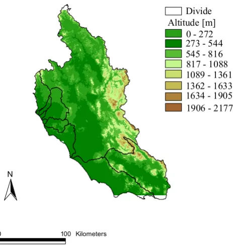
The basins of the target area include the Tiber basin as well as its sub-basins, the basins located in northern Lazio and those located north and south of the Tiber River. These areas show considerable lithological variability affecting the large geomorphological structures.
1192 M. Rianna et al.: Stochastic index model for intermittent regimes The geomorphologic characteristics of the region are
closely connected to the geological domains. In fact, the big geomorphologic domains coincide with recognized ge-ological structures: the big volcanic districts, the Apennine dorsal, the coastal plains and the remaining Tiber valley. In these big geomorphologic structures, it is possible to identify uniformity and therefore distinctive morphotypes.
The hydrographic structure is controlled by the Tiber River system in the northern part of the region and by the river systems in the South of Tiber. The Tiber River basin covers about 17 200 km2and represents the main watercourse of the area.
The Tiber River has an Apennine trend in its initial reach and flows with a torrential regime. Along its right bank, the river collects water from different volcanic districts. From its left bank, it receives water from the Apennine carbon-ate structures. These contributions stabilize the regime. The Tiber River shows a large difference in hydrographic struc-ture between the basins belonging to the right and left banks. This difference is due to the different ways in which the vol-canic systems move, compared to those of carbonate struc-tures characterized by a lower drainage density.
The river basins in the southern part of the study area make up about 4 900 km2and, with the Tiber River, supply the area with 80% of the total runoff. Within these river basins, the permeability characteristics and morpho-topographic struc-tures, mainly represented by carbonate platform deposits, determine the highly effective infiltration and consequently slow development of the hydrographic network and low over-land flow.
The river basins in northern Lazio have been formed on ge-ological formations with low permeability and a hydrge-ological regime characterized by high overland flow from autumn to winter, when their discharges are 3–4 times higher than those in summer.
The karst system is also particularly developed both in the mountains in the north-east area and in the Apennine dorsal, where there are mostly extended karst shapes of large dimen-sion. Moreover, this area has a highly variable climate due to two major bio-climate regions, temperate and Mediterranean, and the relative transitional regions.
The significant differences in the study area are high-lighted in the map of the digital elevation model in Fig. 1, where it is possible to recognize the main basins of the re-gion.
The hydrological data used for the analysis came from the Ufficio Idrografico e Mareografico of Lazio Region. At least 6 years’ worth of daily recorded discharges from 26 stations in the study area were used.
Quantiles Q95, Q50and Q1, were estimated. In particular,
the minimum discharge Q95 is widely used in Europe and
was chosen because of its importance for many applications relating to water management, as in Gustard et al. (1992), Smakhtin (2001) and Laaha and Bloshl (2007).
0 100 Kilometers
N
Altitude [m] 0 - 272 273 - 544 545 - 816 817 - 1088 1089 - 1361 1362 - 1633 1634 - 1905 1906 - 2177 Divide
Fig. 1. Digital elevation model of the study area. The main basins
in the area are divided with black lines.
Each station selected for this study was considered as a separate basin. Thus for basins that do not have upstream stations, the quantiles were calculated directly from the dis-charge data, by adapting the data of each station to the best possible distribution and then calculating the relative quan-tiles. The nested basins were, however, divided into sub-basins separated by several measurement stations; the quan-tiles were calculated as the difference between the quanquan-tiles of the upstream and downstream stations. This last estima-tion is more robust than the quantile calculated from the dif-ference between the hydrographs, but it requires the mean maximum and minimum flow rates to be synchronized in dif-ferent stations. Furthermore, this method reduces the spatial dependence of discharge data (Laaha and Bloshl, 2007). It is necessary to bear in mind that, in the absence of isochrones, error may also be high. All quantiles Q95, Q50and Q1have
also been standardized with respect to the area of the sub-basin to obtain the specific quantiles q95, q50and q1
respec-tively [m3s−1km−2]. Figure 2 shows the geographical rep-resentation of quantiles q1, q50 and q95, where it is evident
that the largest values of specific quantiles are in the South-east of the area that coincides with the Apennine dorsal.
2 2.5 3 3.5 4 4.5 x 10⁵ 4.55 4.6 4.65 4.7 4.75 4.8 4.85
4.9 x 10⁶
East UTM (m)
N or th U TM (m ) 0 0.2 0.4 0.6 0.8 1 1.2 1.4 [m3 s-1 km-2]
2 2.5 3 3.5 4 4.5 5
x 105 4.55 4.6 4.65 4.7 4.75 4.8 4.85
4.9 x 10⁶
East UTM (m)
N or th U TM (m ) 0 0.5 1 1.5 2 2.5 [m3 s-1 km-2]
2 2.5 3 3.5 4 4.5
4.55 4.6 4.65 4.7 4.75 4.8 4.85
x 106 4.9 ) m ( MT Uht ro N 0 2 4 6 8 10
(a) [m3 s-1 km-2] (
x 105 East UTM (m)
b) (c)
2 2.5 3 3.5 4 4.5
x 105 4.55 4.6 4.65 4.7 4.75 4.8 4.85
4.9 x 10⁶
East UTM (m)
N or th U TM (m ) 0 0.2 0.4 0.6 0.8 1 1.2 1.4 [m3 s-1 km-2]
2 2.5 3 3.5 4 4.5 5
x 105 4.55 4.6 4.65 4.7 4.75 4.8 4.85
4.9 x 10⁶
East UTM (m)
N or th U TM (m ) 0 0.5 1 1.5 2 2.5 [m3 s-1 km-2]
2 2.5 3 3.5 4 4.5
4.55 4.6 4.65 4.7 4.75 4.8 4.85
x 106
4.9 ) m ( MT Uht ro N 0 2 4 6 8 10
(a) [m3 s-1 km-2](b)
x 105 East UTM (m)
(c)
2 2.5 3 3.5 4 4.5
x 105 4.55 4.6 4.65 4.7 4.75 4.8 4.85
4.9 x 10⁶
East UTM (m)
N or th U TM (m ) 0 0.2 0.4 0.6 0.8 1 1.2 1.4 [m3 s-1 km-2]
2 2.5 3 3.5 4 4.5 5
x 105 4.55 4.6 4.65 4.7 4.75 4.8 4.85
4.9 x 10⁶
East UTM (m)
N or th U TM (m ) 0 0.5 1 1.5 2 2.5 [m3 s-1 km-2]
2 2.5 3 3.5 4 4.5
4.55 4.6 4.65 4.7 4.75 4.8 4.85
x 106 4.9 ) m ( MT Uht ro N 0 2 4 6 8 10
(a) [m3 s-1 km-2] (
x 105 East UTM (m)
b) (c)
Fig. 2. Geographical representation of specific quantiles q1 (a),
q50 (b) and q95(c). The biggest values of quantiles are located in
the Southeast (Apenninic area), and the dimension of the region of
interest decreases from higher (q1) to lower quantiles (q95). The
black points in the figures represent the gauge stations in the study region.
2 2.5 3 3.5 4 4.5
x 105 4.55 4.6 4.65 4.7 4.75 4.8 4.85
4.9x 10 6
East UTM (m)
N or th U TM (m ) 600 700 800 900 1000 1100 1200 1300 1400 1500 1600 1700 [mm] (a)
2 2.5 3 3.5 4 4.5
x 105 4.55 4.6 4.65 4.7 4.75 4.8 4.85
4.9x 10 6
East UTM (m)
N or th U TM (m ) 5 10 15 20 25 30 35 40 [%] (b)
2 2.5 3 3.5 4 4.5
x 105
4.55 4.6 4.65 4.7 4.75 4.8 4.85
4.9x 10
6
East UTM (m)
N or th U TM (m ) 600 700 800 900 1000 1100 1200 1300 1400 1500 1600 1700 [mm] (a)
2 2.5 3 3.5 4 4.5
x 105
4.55 4.6 4.65 4.7 4.75 4.8 4.85
4.9x 10
6
East UTM (m)
N or th U TM (m ) 5 10 15 20 25 30 35 40 [%] (b)
Fig. 3. Geographical representation of the mean annual
precipi-tation MAP (a) and of the coefficient of variation CV of annual precipitation (b). The black points represent the locations of rain gauges in the region.
precipitation. Again, in this case the orography influences the amount of rainfall over the basin, while the coefficient of variation is lower in the Apennines and higher in the coastal areas. The layout of the digital terrain model, precipitation, variation coefficient and quantiles of the discharge (in par-ticular the maximum) highlight how strongly the orography influences the hydrological behaviour of the region.
Figure 4 shows the basin area against the specific quantile of discharge q1. This scatter plot was used as a preliminary
1194 M. Rianna et al.: Stochastic index model for intermittent regimes
(a)
a
10-2 10-1 100 101 102
0 100 200 300 400 500 600 700
Fiumara Grande
Isola Liri S.angelo theodice
q0 [m3 s-1 km-2]
A
re
a [k
m
2]
q0st-Area
2 2.5 3 3.5 4 4.5
x 105 4.55
4.6 4.65 4.7 4.75 4.8 4.85 4.9x 10
6
East Utm (m)
N
o
rt
h
U
T
M
(
m
)
q0st
Coastal sites Apenninic sites Tiber river sites
East UTM (m) q1[m3s-1km-2]
b
(b)
a
10-2 10-1 100 101 102
0 100 200 300 400 500 600 700
Fiumara Grande
Isola Liri S.angelo theodice
q0 [m3 s-1 km-2]
A
re
a
[k
m
2]
q0st-Area
2 2.5 3 3.5 4 4.5
x 105 4.55
4.6 4.65 4.7 4.75 4.8 4.85
4.9x 10 6
East Utm (m)
N
o
rt
h
U
T
M
(
m
)
q0st
Coastal sites Apenninic sites Tiber river sites
East UTM (m)
q1[m3s-1km-2]
b
Fig. 4. The scatter plot of basin area against specific quantile of
dis-charge q1used as qualitative analysis for preliminary identification
of structures in the dataset (a) (semi-logarithmic representation). It is possible to recognize three different regions. In the figure below
(b), points of the scatter plot are also identified geographically. The
geographical representation points represent the flow level stations.
These groups are formed according to the climatic condi-tions of the area. In particular, it is possible to note how the stations characterized by greater discharges are those in the Apennine region also characterized by higher precipitation depths.
4 Application and results
4.1 Selection of geomorphological variables and correlation analysis
Correlation analysis allows for the evaluation of variables that influence quantiles in the target area.
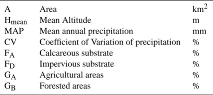
Table 1. Predicting variables and annotation.
A Area km2
Hmean Mean Altitude m
MAP Mean annual precipitation mm
CV Coefficient of Variation of precipitation %
FA Calcareous substrate %
FD Impervious substrate %
GA Agricultural areas %
GB Forested areas %
The choice of characteristics for the basins that were con-sidered for this study was guided by the analysis of the inter-actions among the flow regime, climate and physical charac-teristics.
The geomorphological characteristics were calculated for each basin, using GIS data to obtain the area and maximum height of the basin. The Corine Land Cover (CLC) map, taken from the CORINE program in Lazio and Umbria, was used to evaluate soil use. The hydrogeological map of the area was used to define the percentages of different litholog-ical structures for each basin.
Table 1 shows the variables as well as the symbols used. Table 2 shows the minimum, average and maximum values of some geomorphoclimatic indexes. The characteristics considered are sub-basin area A (km2); the maximum, aver-age and minimum elevation of the basin (Hmax, Hmean, Hmin)
in meters above sea level (m a.s.l.); the value1H = Hmean
– Hminin meters; the percentage of impervious substrate in
the basins (FD); and Mean Annual Precipitation MAP (mm)
calculated for each basin. The values in Table 2 demonstrate the high heterogeneity and complexity of the study region.
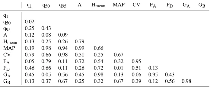
Table 3 shows the correlation matrix estimated for all the dependent variables with data from the study region. Table 4 shows p-values at the 0.05% level when testing the hypothe-sis of no correlation; small p-values indicate significant cor-relation. Table 3 shows that the variables most highly corre-lated with specific quantiles are area, elevation of the basin and lithological characteristics. The correlation of specific quantiles with the area is particularly important. It can be noted that the coefficient diminishes from minimum to max-imum discharges. One hypothesis is that the maxmax-imum dis-charges are influenced not only by the basin area but also by the average rainfall, which causes high flow.
The average annual rainfall influences the maximum dis-charges, which increase as expected when rainfall increases. The coefficient of variation does not appear to affect the dis-charges greatly. The lower disdis-charges are strongly linked to the lithological characteristics of the soil (Nikic and Radonja, 2009).
Table 2. Minimum, average and maximum values of the geomorphological and climatic indexes for the basins in the study region.
A Hmin Hmax Hmean 1H FD MAP
(km2) (m) (m) (m) (m) (%) (mm)
Minimum 31.08 2.00 389.00 32.30 31.30 0.00 650.00
Average 400.05 106.40 1414.60 479.70 396.50 6.53 1066.15
Maximum 981.23 368.00 2200.00 2031.00 2012.00 65.26 1350.00
Table 3. Correlation matrix between discharge quantiles and geomorphological characteristics.
q1 q50 q95 A Hmean MAP CV FA FD GA GB
q1
q50 0.75
q95 –0.34 –0.23
A –0.45 –0.48 –0.49
Hmean 0.42 0.33 0.31 –0.08
MAP 0.34 0.01 0.05 0.00 0.13
CV –0.09 –0.13 0.02 0.19 0.33 0.12
FA 0.58 0.08 0.44 0.11 –0.17 –0.29 0.04
FD 0.20 0.13 –0.44 0.32 –0.11 –0.62 –0.19 0.42
GA 0.21 0.54 0.16 0.22 0.02 0.41 0.52 –0.04 0.22
GB –0.41 –0.26 0.12 –0.32 –0.29 0.12 –0.23 –0.42 0.16 0.02
Table 4. p-value matrix to test the hypothesis of no correlation (critical value equal to 0.05%).
q1 q50 q95 A Hmean MAP CV FA FD GA GB
q1
q50 0.02
q95 0.25 0.43
A 0.12 0.08 0.09
Hmean 0.13 0.25 0.26 0.79
MAP 0.19 0.98 0.94 0.99 0.66
CV 0.79 0.66 0.98 0.51 0.25 0.67
FA 0.05 0.79 0.11 0.72 0.54 0.32 0.95
FD 0.46 0.66 0.11 0.26 0.72 0.01 0.51 0.13
GA 0.45 0.05 0.56 0.45 0.98 0.13 0.06 0.95 0.43
GB 0.13 0.37 0.67 0.25 0.32 0.67 0.39 0.12 0.56 0.98
is probably because higher minimum discharges occur in basins with groundwater flow even in summer. This would also explain the negative correlation with the percentage of impermeable substratum FD. Altitude, on the other hand,
mainly affects maximum discharges. In particular, it was noted that the stations with the highest discharges are those in the Apennines, which are characterised by higher precip-itation depths. This can be explained by the phenomenon of orographic rainfall.
Furthermore, Tables 3 and 4 show large p-values and thus low correlations, probably caused by the wide variability of the study area.
4.2 Cluster analysis through homogeneity test
1196 M. Rianna et al.: Stochastic index model for intermittent regimes It is also necessary to test whether the data observed at
different sites in a homogeneous region arise from a com-mon regional distribution. If the test fails, the association with the region is reconsidered and the procedure is repeated until the region can be considered homogeneous. The two homogeneity tests used were developed by Hosking and Wal-lis (1997) and estimate the degree of heterogeneity of a group of sites in order to evaluate whether they can be considered homogeneous. The tests are based on the L-moment ratios (LCV, L-skewness and L-kurtosis) defined by Hosking and
Wallis (1997).
The first heterogeneity measure is calculated as: H1=
(V−µV)
σV
(10) The H1 measure is based on the sample variance of
L-moment ratio LCV, which Hosking and Wallis (1997)
de-fine as the most significant parameter to individuate homo-geneous regions and here is identified asV.
The parameterV in the H1formulation can be calculated
as:
V= P
ni Lcvi− ¯Lcv 2
P
ni
(11)
whereni is the number of observations in stationi. Licvand ¯
Lcvare the LCVof stationiand the mean regional LCV.
The meanµV and standard deviation σV of the chosen
dispersion measure are estimated using this procedure: the mean regional L-moment ratios are used to evaluate the pa-rameters of a kappa distribution. This allows for the calcula-tion of the repeated simulacalcula-tion of a homogeneous region in which the recorded lengths of its sites are the same as those of the observed data. In this case 500 homogeneous regions were generated. MeanµV and standard deviationσVare then
obtained from these simulations.
The region can be assumed to be homogeneous if the H1
is sufficiently small. Hosking and Wallis (1997) suggest that the region may be assumed to be “acceptably homogeneous” if H1<1, “possibly homogenous” if 1<H1<2 and
“defini-tively heterogeneous” if H1>2.
The H1only measures heterogeneity in the dispersion of
the samples, since it is based solely on the differences be-tween the sample LCV in the region. Hosking and
Wal-lis (1988) also give an alternative heterogeneity measure-ment, which we call H2. It is obtained using the same
pro-cedure as that of H1measurement but is based on LCV and
L-skewness at the same time. H2 has similar acceptability
limits as the H1statistic. Hosking and Wallis (1997) judge
H2 to be inferior to H1, stating that it rarely yields values
larger than 2 even for highly heterogeneous regions. Cluster analysis was then applied, using explanatory vari-ables with the higher correlation coefficient. First of all, the basins’ area, altitudes and geographical coordinates were used to cluster sites. In this way three regions were obtained,
Table 5. Results of the Hosking and Wallis (1997) homogeneity
tests for Q1, mean values Q50and annual minima Q95for the three
regions initially identified.
H1 H2
Tiber Q1 4.008 0.938
Tiber Q50 12.538 1.103
Tiber Q95 1.798 1.815
Coastal Q1 0.043 0.536
Coastal Q50 3.127 0.407
Coastal Q95 2.060 0.649
Appenninic Q1 0.325 0.236
Appenninic Q50 3.003 0.395
Appenninic Q95 3.313 1.178
Region1(Coastal basins)
Region3(TevereRiver,leftbankbasins) Region2(TevereRiver,rightbankbasins)
Region4(Apenninicbasins) N
E W
S
Region 1 (Coastal basins)
Region 2 (Tiber River, right bank basins) Region 3 (Tiber River, left bank basins) Region 4 (Apenninic basins)
Fig. 5. Homogeneous regions recognized in the study area. Four
regions were determined according to the geomorphological char-acteristics of the area.
which coincided with the Apenninic, coastal and Tiber River stations as already identified from the scatter plot. The Hosk-ing and Wallis (1997) homogeneity tests were applied for these regions to the Q1 values, the annual mean values and
Q95values. The results of these tests are depicted in Table 5,
where it can be seen that the more constraining H1statistic
values are often bigger than the threshold value that identi-fies a heterogeneous region. A very high heterogeneity was detected in the Tiber River region in particular. To solve this problem, the percentage of substrate (volcanic or carbonatic) was added to the other variables used to cluster sites and a different configuration of the regions was hypothesized. Af-ter this procedure the Tiber River basins were divided into two regions: the left bank and the right bank of the river. The other two regions coincide with those initially identified.
Figure 5 shows the four regions identified by cluster anal-ysis, while Table 6 shows the results of the two tests for the Tiber River basins after the division. The values for the H1
statistic for the two Tiber regions are lower than in the first configuration; the H2statistic is less than 2 in all cases. The
Table 6. Results of the Hosking and Wallis (1997) homogeneity
tests for annual maxima Q1, mean values Q50and annual minima
Q95for the two Tiber River regions.
H1 H2
Tiber Carbonatic Q1 1.246 0.582
Tiber Carbonatic Q50 2.632 1.239
Tiber Carbonatic Q95 1.842 0.812
Tiber Volcanic Q1 0.124 0.423
Tiber Volcanic Q50 0.764 0.512
Tiber Volcanic Q95 1.314 0.981
River Divide
# Streamgauges
#
# # # #
#
# #
#
# #
0 100 Kilometers
N
1 2
3
4
5 6 7
8
Streamgauges Divide River
100 Kilometers
Fig. 6. Region 4 (Apennine basins), with gauged sites used to
re-gionalize the stochastic index flow model. The red circles high-light the position of the stations used for the testing of the modified stochastic index flow model.
Wallis (1988) showed that regional heterogeneity affects the accuracy of regional flood frequency quantiles more signifi-cantly than does intersite correlation. Hence, because of the great heterogeneity of the region, the tests seem to have been passed.
4.3 Results for the modified stochastic index flow model
A more thorough description is shown here for the procedure of the modified stochastic index flow model. Only two sta-tions (nos. 3 and 5) with an intermittent regime were avail-able in the study region, both of which were located in the Region 4 (Apennine basins). Figure 6 shows the Apennine area and the two sites considered in the analysis. Seven years of data, from 2003 to 2010, are available for sites nos. 3 and 5. Initially AF andX0 were calculated for each time series, and several distributions were fitted to these series to calculate the FDC using the stochastic index flow model.
First the FDC was calculated using the stochastic index flow model, without using the theory of total probability. Then the new model was used to calculate FDC when zero data were present. The probability of non-zero flowpnzand
the complementpdrywere calculated for both sites and then
zero data were separated from the time series. pnzwas 95%
10-3 10-2 10-1 100 101
0.0005 0.001 0.005 0.01 0.05 0.1 0.25 0.5 0.75 0.9 0.99 0.999 0.9999
Discharge [m3/s]
Pr
o
b
a
b
il
it
y
Weibull Weibull
0 10 20 30 40 50 60 70 80
0.5 0.95 0.99 0.995 0.999 0.9995
Discharge [m3/s]
Pr
ob
ab
ili
ty
Weibull
L-moments GEV max
(a)
(b)
Fig. 7. Fitted Conditional Frequency Distribution FX0nz= Pr(X0≤
x0|X06=0) for sites n. 5 (a) (logarithmic representation) and n. 3
(b). The best distributions are the Weibull distribution for site n. 5 (a) and GEV max with parameters obtained with the L-moment
method for site n. 3 (b).
and 97% for sites nos. 3 and 5, respectively. These values were calculated using the standard plotting position formula-tion.
Subsequently, a fitting procedure was applied to the non-zero data. Empirical distribution for AF and X0 was cal-culated using the formulation that considers only non-zero data. Normal distribution is the best distribution for AF non-zero data. Figure 7 represents the fitting of distributions for X0 non-zero data. The distributions that fit the values best
were the Weibull distribution forX0non-zero data from sta-tion no. 5 and GEV Max with parameters obtained using L-moments forX0data without zero from station no. 3.
Computation of conditional distribution FAFnz =
Pr(AF≤af|AF6=0) and fX0nz = Pr X0≤x0|X06=0 with positive values of the series was then performed.
1198 M. Rianna et al.: Stochastic index model for intermittent regimes
0 10 20 30 40 50 60 70 80 90 100
10-2
100
Duration [%]
D
is
ch
ar
ge
[m
3/s]
Empirical FDC
Modified stochastic index model Stochastic Index model
0 10 20 30 40 50 60 70 80 90 100
10-3
10-2
10-1
100
101
Duration [%]
D
is
ch
ar
ge
[m
3/s
]
Empirical FDC
Modified stochastic index model Stochastic index model
(a)
(b)
Fig. 8. Semi-logarithmic representation of fitted FDC (Pr(X > x))
for sites n. 5 (a) and n. 3 (b). The broken black line is the empirical FDC, obtained through the Weibull plotting position, the solid grey line is calculated using the modified stochastic index flow model and the broken bright grey line is FDC calculated using the standard stochastic index flow model.
Figure 8 represents the FDC for the two stations. The re-sults are represented on a semi-logarithmic scale.
In order to evaluate the accuracy of the modified model, the Root Mean Square Error (RMSE) and Nash-Sutcliffe (NS) efficiency coefficient were calculated.
The formulation of RMSE is:
RMSE= v u u u t
n
P
i=1
Qt o−Qtm
2
n (12)
whereQtois the observed discharge at the timet, andQtmis modelled discharge at timet.
The formulation of the Nash-Sutcliffe efficiency coeffi-cient is:
NS=1−
T
P
t=1
Qto−Qtm
T
P
t=1
Qt o−Qo
(13)
whereQois the mean value of the observed discharges.
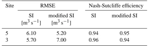
Table 7. RMSE and Nash-Sutcliffe efficiency calculated for the two
stations with intermittent regime and for the standard and modified formulation of the stochastic index flow model. The Nash-Sutcliffe efficiency is calculated on logarithms of data.
Site RMSE Nash-Sutcliffe efficiency
SI modified SI SI modified SI
[m3s−1] [m3s−1]
5 6.10 5.20 0.94 0.95
3 5.70 7.00 0.96 0.94
Nash-Sutcliffe efficiencies can range from−∞to 1. An efficiency value of 1 (NS = 1) represents a perfect match of the modelled discharges to the observed data. An efficiency value of 0 (NS = 0) indicates that the model’s predictions are as accurate as the mean of the observed data, whereas an efficiency less than zero (NS<0) occurs when the observed mean is a better predictor than the model.
Results for RMSE and NS efficiency are shown in Table 7 for the stations with an intermittent regime. These efficiency indexes are calculated for the FDC using both the stochastic index flow model in the standard formulation and the mod-ified model. The results from the modmod-ified stochastic index flow model are better than those from the standard formu-lation for the station no. 5, while they are worse for station no. 3. The modest difference between the two curves (calcu-lated using the standard and the modified formulations) de-pends on the small percentage of zero values in the dataset. Moreover, the performance of the modified stochastic index flow model for station no. 3 is probably affected by the par-ticular shape of the empirical curve, due to over-abstraction of groundwater.
4.4 Regionalisation analysis
4.4.1 Choice of the best parent distribution for AF andX0
To develop a regionalisation model, all the sites must have the same parent distribution; it is then necessary to choose distributions that closely fit AF andX0data for all stations. It is also important to choose the distributions with the fewest parameters in order to have a parsimonious model.
The analysis was carried out in Region 4, which corre-sponds to the Apennine region and comprises eight stations (Fig. 6). The regionalisation approach was tested in this re-gion involving basins with intermittent flow. Six out of the eight sub-basins are considered to have a permanent regime. For this reason, the stochastic index flow model was applied to these stations with the classical implementation. This means that for these stations the value ofpnz is 1 because
0 10 20 30 40 50 60 70 80 90 100
101
102
Duration [%]
D
is
c
h
a
rg
e
[
m
3/s
]
Stochastic index model Empirical FDC
Fig. 9. Results of application of the stochastic index flow model
for site n. 8 (semi-logarithmic representation). The broken black line represents the empirical FDC; the grey line represents the FDC obtained with the stochastic index flow model.
For AF values of the different sites, several distributions have a good fit. The best distribution for the data was the nor-mal one. This result was expected because of the low skew-ness of the annual flow and the central limit theorem. More-over, this distribution has only two parameters, the meanµ and standard deviationσ.
To evaluate the best distribution for X0 data, a method based on the moment ratio diagram that represents L-skewness versus L-kurtosis was used. Figure 10 demon-strates that the GEV distribution gives the best fit for almost all the stations. Observed parameters from the sites of the region are provided in Table 8.
A regression model was used to transfer model parameters to ungauged basins (see Sect. 4.4.2). Parameters of normal distribution as well as scale parameterλand shape parameter κof the GEV distribution are estimated by equations depen-dent on geomorphological characteristics. It is possible to evaluate location parameterξ of the GEV distribution using L-moment formulation (Hosking and Wallis, 1997). λ1, the
mean value of the standardized discharge sampleX0, is equal to unity. Location parameterξcan thus be evaluated after the estimation ofκandλparameters:
λ1=ξ+λ{1−0 (1+κ)}/κ. (14)
where0(.)represents the gamma function.
The other parameter of the model is thepnzvalue that
eval-uates the regime type of the basin and can range from 0 for basins with no flow in the period of measurements to 1 for rivers with permanent regimes.
4.4.2 Regression models
Stepwise regression analysis was performed for all stations in the region. For this type of statistical regression model, the order of entry of the predictor variables is based on an F-test.
0 0.1 0.2 0.3 0.4 0.5 0.6 0.7 0.8 0.9 1
0 0.2 0.4 0.6 0.8 1
L-skewness
L-ku
rt
os
is
GEV GLO GPD GUM LNO NOR PE WEI Sample L-moments
Fig. 10. L-moment ratio diagram of L-kurtosis vs. L-skewness,
used to choose the parent distribution. Distributions in the diagram are: Normal (NOR), Gumbel (GUM), Generalized extreme values (GEV), Generalized logistic (GLO), Generalized Pareto (GPD), Generalized normal (LNO), Pearson type III (PE), Weibull (WEI).
Table 8. Observed parameters for the stations of Region 4
(Apen-nine area) used for the regionalisation approach. µandσ are the
mean and standard deviation of the AF data;κ,λandξare the shape
parameter, scale parameter and location parameter of the GEV
dis-tribution of theX0data;pnzis the percentage of time that the river
is flowing.
µ σ κ λ ξ pnz
Site 1 20.26 3.03 0.33 0.16 0.83 100.00
Site 2 6.44 1.38 0.29 0.24 0.77 100.00
Site 3 0.04 0.02 0.57 0.32 0.40 95.00
Site 4 5.73 3.89 2.25 0.16 0.07 100.00
Site 5 1.12 0.49 2.01 0.15 0.08 97.00
Site 6 8.95 1.47 0.35 0.22 0.76 100.00
Site 7 36.47 4.88 0.26 0.10 0.91 100.00
Site 8 76.94 25.39 0.51 0.29 0.58 100.00
A validation analysis, through jack-knife procedure, is then necessary to evaluate the accuracy of the regional es-timates. This method allows a simulation of the presence of ungauged basins and is assessed using the procedure below (Castellarin et al., 2004).
One of the stations of the homogeneous region was re-moved from the sample and a new regression analysis was carried out without it. New parameters were then calculated for this station with the new equations; the results were used to calculate the FDC. The procedure was then applied to all the stations.
The stepwise procedure was then used to define regionali-sation models to calculate the five parameters in ungauged basins. Three kinds of models (linear, exponential and logarithmic) were evaluated:
ˆ
1200 M. Rianna et al.: Stochastic index model for intermittent regimes
ˆ
ϑ=A0·ωA11·ω2A2·ωnAn+ϑ; (16)
ˆ
ϑ=A0+ln(A1·ω1)+ln(A2·ω2)+ln(Anωn)+ϑ. (17)
whereϑˆ is the perfect estimated parameter,Ai,i=1,2,...,n
are the coefficients of the model,ωi are the explanatory
vari-ables andϑis the residual of the models.
The regression models identified for the five parameters of the modified stochastic index flow model are:
µ=A0·
AA1·FA2 A
; (18)
σ =A3·
AA4; (19)
κ =A5·
FDA6
·HA7; (20)
λ=A8·
AA9; (21)
pnz=A10·
FDA11
·AA12. (22)
The two parameters of the AF data depend on the area of basin A, while parameters of theX0 data andpnz also
de-pend on the percentage of pervious substrate FDand on the
percentage of calcareous substrate FA.
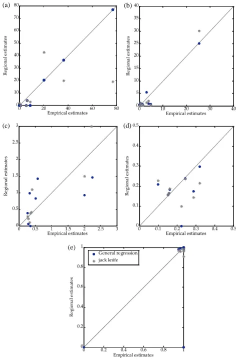
Figure 11 shows the scatter plots of parameters observed versus the parameters predicted, which were calculated from all sites using the jack-knife procedure. It can be seen that the parameters estimated using the jack-knife procedure are more scattered than those obtained with general regression; however, they are not so different as to imply that the models cannot be used.
4.4.3 Results of regionalisation
The flow duration curves calculated using parameters ob-tained through jack-knife validation were then compared with empirical FDC in order to evaluate the accuracy of the model.
To evaluate the performance of the model, the following indicator was considered (Castellarin et al., 2004):
εs,j=
ˆ
qs,j−qs,j
qs,j
·100 (23)
whereqs,j andqˆs,j indicate the daily streamflow, empirical
and estimated through regionalisation, associated with dura-tionjfor stations. From these values it is possible to obtain the mean relative errorε¯sand its standard deviationσε,sfor a
station as:
¯
εs=
1 N0·
N0
X
j=1
εs,j (24)
σε,s= v u u t
1 N0 ·
N0
X
j=1
εs,j− ¯εs 2
(25)
0 0.2 0.4 0.6 0.8 1
0 0.2 0.4 0.6 0.8 1 Empirical estimates Re gi on al e st im at es General regression jack knife
0 20 40 60 80
0 10 20 30 40 50 60 70 80 Empirical estimates Re gi on al e st ima te s
0 10 20 30 40
0 5 10 15 20 25 30 35 40 Empirical estimates Re gi on al e st im at es
0 0.5 1 1.5 2 2.5 3
0 0.5 1 1.5 2 2.5 3 Empirical estimates Re gi on al e st ima te s
0 0.1 0.2 0.3 0.4 0.5
0 0.1 0.2 0.3 0.4 0.5 Empirical estimates Re gi on al e st im at es (a) (b) (c) (d) (e)
Fig. 11. Scatter plot of observed parameters vs. predicted
parame-ters of the stochastic index flow model. Graphs (a) and (b) represent
µandσ parameters of the normal distribution. Graphs (c) and (d)
representκandλparameters of the GEV distribution, and Graph
(e) is the scatter plot of thepnzvalues (in probability form).
whereN0represents the number of durations that are consid-ered to calculate mean and standard deviation.
In addition, the average ofNvalues of Eq. (24),ε, and of¯
Eq. (25),σε, withN corresponding to the number of sites,
gives an indication of the performance of the model. It is also possible to graphically represent the mean and median of the distribution of theNrelative errorsεi,jand the
100(α/2) % and 100[1−(α/2)] % percentiles, by identifying the interval about the median containing the 100(1−α) % of theN relative errors, against durationsj, to evaluate the uncertainty of the regional FDC for all durations.
The mean relative error for a given durationj can be cal-culated as:
¯
εj=
1 N
N
X
i=1
0 10 20 30 40 50 60 70 80 90 100
10-3
10-2
10-1
100
101
102
103
Duration [%]
D
is
c
h
a
rg
e
[
m
3/s
]
jack knife FDC Empirical FDC
0 10 20 30 40 50 60 70 80 90 100
10-1
100
101
102
Duration [%]
D
is
c
h
a
rg
e
[
m
3/s
]
jack knife FDC Empirical FDC
(a)
(b)
Fig. 12. Semi-logarithmic representation of empirical and
jack-knife FDC for site n. 5 (intermittent regime) (a) and for site n. 1 (permanent regime) (b).
Another performance indexEsthat can be used is the
Nash-Sutcliffe efficiency method, calculated for each station as:
Es=1− N0
P
j=1 ˆ
qs,j−qs,j
2
N0
P
j=1
qs,j− ¯qs 2
(27)
whereqˆs,jis the estimated value for each durationj and site
s,qs,j is the empirical value for each duration j and site s
andq¯s is the mean value. The value of this index can range
between 1 and−∞.
TheEs values are used to calculate three indexes of the
effectiveness of the model:
– P1is defined as the percentage of cases overNstations
in whichEs>0.95;
– P2is defined as the percentage of cases overNstations
in which 0.50< Es<0.95;
– P3is defined as the percentage of cases overNstations
in whichEs<0.5.
0 10 20 30 40 50 60 70 80 90 100
-10 0 10 20 30 40 50 60
Duration [%]
R
e
la
ti
ve
E
rr
or
[
%
]
Mean Error Median Error Percentile 10% Percentile 90%
Fig. 13. Representation of mean (solid black line), median (solid
grey line) and 10% and 90% percentiles (broken grey and black lines) of relative error for different durations.
Table 9. Indexes of reliability calculated on FDC obtained from the
regionalisation model.
¯
εs[%] 0.96
σε[%] 3.68
P1[%] 0.54
P2[%] 0.18
P3[%] 0.27
Figure 12 shows FDC results for two explanatory sites. Ta-ble 9 shows the results of the average relative error and the standard deviation of relative error for the region and the Nash-Sutcliffe efficiency index. Figure 13, on the other hand, is a graphic representation of mean, median and 10% and 90% percentiles of relative errors.
The relative error graph shows that the worst results are produced for shorter durations, but the error decreases; for durations greater than 20%, it is lower than 1%. The median value is less affected by the anomalous values and is always under 1%, very near 0%. It is particularly important to note that the relative error calculated for the higher percentage of durations, which coincides with the lower part of the FDC, is very low. The efficiency results are quite good: in fact, more than 50% of the sample is very well fitted, and only 27% fits poorly.
5 Summary and conclusions
The principal aim of this paper is to create a method for cal-culating FDC in the presence of zero data caused by zero flow in basins with intermittent regime, where environmen-tal problems caused by wastewater are critical.
1202 M. Rianna et al.: Stochastic index model for intermittent regimes by Castellarin et al. (2004), in that it utilizes the theorem
of total probability. This is used to calculate the probabil-ity of all data Pr(X≤x), while the stochastic index flow model is used to calculate the conditional distribution Pr(X≤
x|X6=0).
The method is introduced in a context of regionalisation; consequently, a procedure to transfer this model has been proposed. The starting point is the definition of homoge-neous regions in the study area using cluster analysis and geomorphological variables as explanatory variables. Multi-ple regression analysis then brought about the definition of certain equations needed to transfer hydrological informa-tion to ungauged basins. At the end, an evaluainforma-tion through jack-knife validation was performed to simulate the use of the model in the case of ungauged basins.
The definition of homogeneous regions was applied to basins in Central Italy and the modified stochastic index flow model was tested in a homogeneous region involving basins with intermittent flow.
Moreover, from the preliminary analysis of the discharge, four groups of nearby stations were identified. The factors with the most influence on the similarity of the data are the average altitude of the basin, the climate, the proximity of the observed stations to the coastline and the type of sub-strate. Cluster analysis using these geomorphological char-acteristics was then applied, and four corresponding regions were found according to the climatic condition of the area. The preliminary analysis showed a high heterogeneity in the area, caused by the orography that influences the climate and by the different types of substrate.
The results of the application of the five-parameter model show that it can be used to represent FDC on rivers with zero flow. In fact, the application of the modified model has produced a better approximation of FDC for one of the two stations analysed. Although a worse result is provided for the other one, this is probably caused by over-abstraction of groundwater. Furthermore, the little difference between the two models is due to the small percentage of zero data. Surely an application to a larger number of basins, character-ized by a significant number of zero values, would be neces-sary to better evaluate the performance of this technique.
The regionalisation of the model and the jack-knife valida-tion also provided good results. The implementavalida-tion of the regionalisation model shows that the approach used based on the regression relationships and identified through step-wise regression relationships, can be adopted in different geographical areas by simply changing the explicative vari-ables. It is important to underline that both the regionalisa-tion approach and the validaregionalisa-tion were applied to a modest sample, since there was only one region in the study area with intermittent gauging stations. Only a few stations were thus used, of which only two had zero flow. Hence, further studies are necessary to test the model’s applicability in re-gions with more stations with zero flow. Furthermore, the nested structure of the region influences the results of both
the homogeneity tests and the regression models. Therefore, further work should develop a procedure to regionalise the model in regions characterized by nested structures and cre-ate a model to compute annual-based FDC in intermittent rivers.
Acknowledgements. The authors thank anonymous reviewer and
Andreas Efstratiadis for their helpful comments.
Edited by: R. Deidda
Reviewed by: A. Efstratiadis and another anonymous referee
References
Castellarin, A., Vogel, R. M., and Brath, A.: A stochastic index flow model of flow duration curves, Water Resour. Res., 40, W03104, doi:10.1029/2003WR002524, 2004.
Cigizoglu, H. K. and Bayazit, M.: A generalized seasonal model for flow duration curve, Hydrol. Process., 14(6), 1053–1067, 2000. Claps, P. and Fiorentino, M.: Probabilistic flow duration curves for
use in environmental planning and management, in: Integrated Approach to Environmental Data Management Systems, edited by: Harmancioglu, N. B., Alpaslan, M. N., Ozkul S. D., Singh,, V. P., Kluwer Academy, NATO ASI Series, Ser. 2(31), 255–266, 1997.
Dalrymple, T.: Flood frequency analyses, US Geological Survey, Water Supply Papers, 1543-A, 1960.
Durrans, S. R., Ouarda, T. B. M. J., Rasmussen, P. F., and
Bob´ee, B.: Treatment of zeroes in tail modelling of low
flows, J. Hydrol. Eng., 4(1), 19–27, doi:10.1061/(ASCE)1084-0699(1999)4:1(19), 1999.
Ganora, D., Claps, P., Laio, F., and Viglione, A.: An approach to estimate nonparametric flow duration curves in ungauged basins, Water Resour. Res., 45, W10418, doi:10.1029/2008WR007472, 2009.
Gustard, A., Bullock, A., and Dixon, J. M.: Low flow estimation in the United Kingdom, Institute of Hydrology, Wallingford, UK, Report n. 108, 1992.
Haan, C. T.: Statistical methods in hydrology, Iowa State University Press, Ames, Iowa, 1977.
Hosking, J. R. M. and Wallis, J. R.: The effect of inter-site depen-dence on regional flood frequency analysis, Water Resour. Res., 24(4), 588–600, doi:10.1029/WR024i004p00588, 1988. Hosking, J. R. M. and Wallis, J. R.: Regional frequency analysis,
Cambridge University Press, New York, 1997.
Jennings, M. E. and Benson, M. A.: Frequency curve for annual flood series with some zero events or incomplete data, Water Resour. Res., 5(1), 276–280, doi:10.1029/WR005i001p00276, 1969.
Kilmartin, R. F. and Peterson, J. R.: Rainfall-runoff regression with logarithmic transforms and zeros in the data, Water Resour. Res., 8(4), 1096–1099, doi:10.1029/WR008i004p01096, 1972. Kroll, C. N. and Stedinger, J. R.: Estimation of moments and
quan-tiles using censored data, Water Resour. Res., 32(4), 1005–1012, 1996.
LeBoutillier, D. V. and Waylen, P. R.: A stochastic model of flow duration curves, Water Resour. Res., 29(10), 3535–3541, doi:10.1029/93WR01409, 1993.
Mimikou, M. and Kaemaki, S.: Regionalization of flow duration characteristics, J. Hydrol., 82(1–2), 77–91, doi:10.1016/0022-1694(85)90048-4, 1985.
Nikic, Z. and Radonja, P.: Modelling the influence of hydro-geological parameters on low flow in hilly and mountain-ous regions of Serbia, Hydrolog. Sci. J., 54(3), 484–496, doi:10.1623/hysj.54.3.484, 2009.
Quimpo, R. G., Alejandrino, A. A., and McNally T. A.: Re-gionalised flow duration curves for Philippines, J. Water Res. Pl.-ASCE, 109(4), 320–330, doi:10.1061/(ASCE)0733-9496(1983)109:4(320), 1983.
Searcy, J. C.: Manual of hydrology 2, Low flow techniques, flow du-ration curves, US Geological Survey, Water Supply Paper, 1542-A, 1959.
Smakhtin, V. U.: Low flow hydrology: a review, J. Hydrol., 240, 147–186, 2001.
Smakhtin, V. Y., Hughes, D. A., and Creuse-Naudine, E.: Region-alization of daily flow characteristics in part of the Eastern Cape, South Africa, Hydrolog. Sci. J., 42(6), 919–936, 1997.
Strupczewski, W. G., Weglarczyk, S., and Singh, V. P.: Impulse re-sponse of the kinematic diffusion model as a probability distribu-tion of hydrologic samples with zero values, J. Hydrol., 270(3– 4), 328–35, doi:10.1016/S0022-1694(02)00309-8, 2003.
Subcommittee on Hydrology: Methods of Flow Frequency Analy-sis, Inter-Agency Committee on Water Resources, Notes on hy-drological act, Bulletin 13, Washington D.C., April 1966. Tate, E. L. and Freeman, S. N.: Three modelling approaches for
seasonal droughts in southern Africa: the use of censored data, Hydrolog. Sci. J., 45(1), 27–42, 2000.
Vogel, R. M. and Fennessey, N. M.: Flow duration curves:
new interpretation and confidence intervals, J. Water Res.
Pl.-ASCE, 120(4), 485–504,
doi:10.1061/(ASCE)0733-9496(1994)120:4(485), 1994.
Wang, C. Y. and Singh, R. P.: Frequency estimation for hydrological samples with zero data, J. Water Res. Pl.-ASCE, 121(1), 98–108, doi:10.1061/(ASCE)0733-9496(1995)121:1(98), 1995. Ward J. H.: Hierarchical grouping to optimize an objective function,
J. Am. Stat. Assoc., 58(301), 236–244, doi:10.2307/2282967, 1963.
Woo, M. K. and Wu, K.: Fitting annual floods with zero flows, Can. Water Resour. J., 14(2), 10–16, 1989.
Yu, P. S., Yang, T. C., and Wang, Y. C.: Uncertainty analysis of regional flow duration curves, J. Water Res. Pl.-ASCE, 128(6),
424–430, doi:10.1061/(ASCE)0733-9496(2002)128:6(424),