Article
1
Unsupervised Feature Learning in Time Series
2
Prediction Using Continuous Deep Belief Network
3
Qili Chen
1*, Guangyuan PAN
2*, Ming Yu
3, Jiuhe Wang
14
1 Automation college at Beijing information science and technology University, Beijing, China;
5
6
2 Civil & Environmental Engineering at University of Waterloo , Waterloo, Canada; [email protected]
7
3 Electronic Engineering at The Chinese University of Hong Kong, Hong Kong SAR, China
8
* Correspondence: [email protected]; Tel.: +1-226-978-9816
9
10
Featured Application: We have specific interests on using DBN, a deep learning model, for
11
parameters predicting in environmental protection industries, not only because of the previous
12
promising results, but also the beauty in DBN’s unsupervised learning algorithm. In this paper, we
13
also aim to analyze the model characteristics and extend its potential usages. By improving the
14
unsupervised learning process algorithm, the proposed model now can process continuous data in
15
a better way. In the experiments, we find that the model outperforms many other existing ones
16
including the traditional DBN.
17
Abstract: A continuous Deep Belief Network (cDBN) with two hidden layers is proposed in this
18
paper, focusing on the problem of weak feature learning ability when dealing with continuous data.
19
In cDBN, the input data is trained in an unsupervised way by using continuous version of transfer
20
functions, the contrastive divergence is designed in hidden layer training process to raise
21
convergence speed, an improved dropout strategy is then implemented in unsupervised training to
22
realize features learning by de-cooperating between the units, and then the network is fine-tuned
23
using back propagation algorithm. Besides, hyper-parameters are analysed through stability
24
analysis to assure the network can find the optimal. Finally, the experiments on Lorenz chaos series,
25
CATS benchmark and other real world like CO2 and waste water parameters forecasting show that
26
cDBN has the advantage of higher accuracy, simpler structure and faster convergence speed than
27
other methods.
28
Keywords: Unsupervised training; Features learning; Deep learning; Time series forecasting
29
30
1. Introduction
31
Deep Belief Network (DBN) has been popularly focused on around the world since its good
32
abilities in image and acoustic recognition tasks [1]. By simulating the cognitive and knowledge
33
reference processes of human brain, DBN is famous for its special training method which is called
34
greedy unsupervised training [2]. By stacking several Restricted Boltzmann Machines (RBM) one
35
upon another in this process, DBN learns the features of input signals supervisor needlessly to obtain
36
a better distributed representation, without requiring extra data with labels on it like Back
37
Propagation [3]. Instead, DBN combines the processes of feature learning and supervised training
38
together, avoiding features been selected manually and incorrectly [4]. The essence that the process
39
of unsupervised training is in fact the weights initialization for supervised training is put forward
40
[5]. Weights can be selected and trained into a very good area and ensure the step of supervised
41
training more effective and faster than weights random initialization [6]. Nowadays, based on this
42
philosophy, more and more Deep Neural Network models have been proposed and new records
43
have been achieved in AI, especially in pattern recognition, such as feature extraction, voice
44
recognizing, document categorization, semantic understanding, and so on [7-12].
45
Although it has achieved lots of improvements, DBN works in a way of data discretization in
46
extracting features, thus all the visible and hidden units are Bernoulli values. Hence, little
47
achievement and application of using DBN in industry area is published [13]. For example, a satisfied
48
accuracy cannot be realized in time series forecasting tasks in data collection and detection systems
49
[14]. Although many other deep learning models, such as convolutional neural networks (especially
50
pretrained models), LSTM and deep reinforcement learning are able to process continuous data in
51
time series prediction, DBN does not performs well in this application [33-34]. The driving force
52
behind this research is that DBN is sounded for its feature learning ability and unsupervised learning,
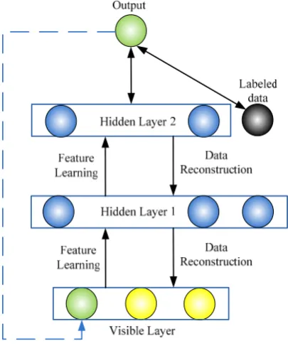
53
the real-world applications especially time series prediction will benefit from DBN’s data processing
54
ability.
55
The contributions of this paper are follows.
56
• First, to increase DBN’s ability of processing continuous data, a continuous Deep Belief
57
Network (cDBN) with two hidden layers is proposed in this paper, to realize modelling time
58
series data in industries applications.
59
• Second, some training technics are improved, and their effectiveness are analysed, for
60
example, Contrastive Divergence (CD) is implemented to train one hidden layer at a time;
61
the output of the first RBM is set to be the input of the second RBM. In the unsupervised
62
training process, an improved strategy of dropout in unsupervised learning is implemented
63
to reduce over fitting by preventing co-adaptation of feature detectors, and this strategy helps
64
to learn features intelligently and wisely because it reduces a neuron’s dependency on others.
65
• Third, through stability analysis, the stability theorem is put forward to provide
hyper-66
parameters-selecting.
67
• Finally, this cDBN is tested in two kinds of experiments; simulation experiments, for
68
example, Lorenz chaos series and Competition on Artificial Time Series (CATS) benchmark,
69
and real-world applications such as atmospheric oxygen carbon (CO2) forecasting and
70
wastewater parameter prediction. The results show that it has higher accuracy, simpler
71
structure, and better stability of using cDBN.
72
The following parts are designed as: Section 2 is the related works done by other researchers and
73
us before. Section 3 describes the structure and algorithm of proposed cDBN, Section 4 introduces an
74
improved dropout strategy for unsupervised learning, Section 5 is stability analysis, Section 6 shows
75
the experiments using cDBN, and the final section gives the conclusions of this study.
76
2. Related Works
77
Researchers have done many significant works towards realising continuous deep belief
78
network in time series prediction. Hinton proposes a method to receive and process continuous data
79
for visible layer, however those visible and hidden units can still only deal with Bernoulli values in
80
unsupervised training [15]. The author of [16] analyses the theory of training a Restricted Boltzmann
81
Machine, and shows it has the ability of processing continuous data and can be used in network
82
modelling. More approaches have been achieved recently by [17], in which an improved RBM, whose
83
transfer function is changed to be able to process continuous data, is used to predict stock changing.
84
By trying different numbers of units and layers, a satisfied prediction is realized. Besides, in order to
85
solve the problem of co-adaptation in training, the strategy of dropout is proposed [18], this strategy
86
drops units randomly in supervised training, and this prevents complex co-adaptations of feature
87
detectors in hidden units, insuring that a unit can be helpful and independent in the context with
88
several other specific feature detectors. But the problem of low effectiveness of feature learning in
89
unsupervised training is still severe, especially in time series predicting tasks [19]. Kuremoto uses
90
Particle Swarm Optimization (PSO) to calculate the number of hidden layer units before designing
91
the structure of a DBN, however, this method still needs to pre-set a certain size for hidden layers,
92
also it is still time consuming [20].
We have also done some previous researches towards this direction. In [35], a special
94
regularization-reinforced term is developed to make the weights in the unsupervised training process
95
to attain a minimum magnitude. Then, the non-contributing weights are reduced, and the resultant
96
network can represent the inter-relations of the input-output characteristics. Using this method, the
97
optimization process is able to obtain the minimum-magnitude weights of DBN. In [36-37], we
98
attempt to demonstrate the potential of this new model for crash prediction using DBN, the
99
continuous version transfer function and the technic of regularization are carefully studied.
100
According to these previous studies, DBN has been proved to have the potential for processing
101
continuous data by benefiting its feature learning ability. So, in this paper, we will move on to
102
demonstrate the developing method.
103
3. Methodology
104
3.1 The structure of cDBN
105
An illustration of the proposed cDBN is shown in Fig 1. This cDBN consists of 4 layers. The first
106
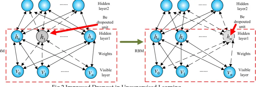
layer is visible layer (V) which receives the original time series data at time t, (t-1) … (t-n), so it’s
107
the input of cDBN. V is followed by two hidden layers, L1 and L2. V and L1 formed the first RBM,
108
and L1 and L2 make up the second one. The structure of each RBM is that of a two-way full
109
connectivity between V and L (as shown by double sided arrows). No connections exist between units
110
of the same layer. The absence of intra-layer connections results to a “restricted” Boltzmann Machine.
111
In the training process, each hidden layer extracts the last layer’s data information and feature to
112
form a better although more abstract distributed representation of input data. The last layer is output
113
which is only one unit. This layer also means another feature that has been learnt from input, and its
114
mathematical meaning is the predicted value at time (t+1). The reason why two hidden layers are
115
recommended is on traditional DBN, two layers are good enough in a pattern reorganization task,
116
and they are definitely more powerful in extracting features than only one layer used [21-22], besides,
117
multi layers will be time consuming for industries and real-world applications.
118
119
Fig 1 Continuous DBN’s Structure
120
As DBN must transit the original signal to be Bernoulli values when processing, its applications
121
are limited. Hinton improved its visible layer to receive continuous values, while the signal in the
122
unsupervised training process will still be transited to Bernoulli value [15]. According to previous
123
work that has been done by Bengio, RBM is capable of processing continuous data and modelling in
124
theory [16]. Furthermore, some recent works have shown that continuous RBM can be used in stock
prediction [23]. A continuous RBM is put forward to predict water parameters in Huai River in China
126
and gets good results in [24]. In the study of [20], particle swarm optimization (PSO) is used to select
127
the best structure for DBN, and then the unit-amount-selected DBN is used in the task of CATS
128
benchmark, good results are obtained. Based on the works that have been done, the transfer functions
129
in DBN are improved to process continuous data in this paper, and then an improved dropout in the
130
training process is studied.
131
3.2 The training processes of cDBN
132
DBN is made of several RBMs, which are trained separately before unfolding the whole network
133
to use back propagation in weights’ fine tuning. So DBN is a kind of recurrent neural network that
134
combines unsupervised and supervised learning together. The knowledge learning and reasoning
135
processes in a RBM, which can be called knowledge generation, are shown in formulas (1) and (2).
136
𝑝 ℎ = 1 =
∑(1)
137
𝑝(𝑣 = 1) =
∑(2)
138
where vi is the value of unit i of visible (input) layer, hj is the value of j in hidden (output of RBM)
139
layer. b and c stand for the biases of visible and hidden layers respectively. wij is the weight between
140
visible unit i and hidden unit j. Define θ=(W,b,c), then according to Contrastive Divergence [25] the
141
formula of renewing weights and biases is shown as follows.
142
𝜃
( )=< ℎ 𝑣 > −< ℎ 𝑣 >
(3)
143
where <> denotes the average over the sampled states, hj0 vi0 means the state of visible layer
144
multiples hidden layer at the beginning, and hj1 vi1 means the same except both layers have ran
145
Markov chain once.
146
While in cDBN, the transfer functions will be improved to process continuous data. Let sj and si
147
be the values of hidden unit j and visible unit i, and the sigmoid function in (1) and (2) will be kept,
148
while the step of discretization is omitted. After that, an item of noise function will be added to realize
149
the transformation.
150
𝑠 = 𝜑 (∑ 𝑤 𝑠 + 𝜎 ∙ 𝑁 (0,1))
(4)
151
𝑠 = 𝜑 (∑ 𝑤 𝑠 + 𝜎 ∙ 𝑁 (0,1))
(5)
152
At the same time,
153
𝜑 𝑥 = 𝜃 + (𝜃 − 𝜃 ) ∙
(6)
154
𝜑 (𝑥 ) = 𝜃 + (𝜃 − 𝜃 ) ∙
(7)
155
156
(4) and (5) are the processes of learning and generating, in which, N(0,1) is a Gaussian random
157
variable with mean 0 and variance 1. σ is a constant, and φ(∙) denotes the sigmoid function with
158
asymptotes θH and θL. a is a variable that controls noise, which means it controls the gradient of
159
transfer function.
160
4. Improved unsupervised learning
161
When a large size of cDBN is trained on a small training set, it typically performs poorly on
held-162
out test data. This is because of over fitting, which means the network is trained to accurately
163
recognize the examples presented in the training as separate cases ignoring possible associations
164
between them, and the feature detectors (hidden units) have been tuned to work well together on the
165
training data but not on the test data. Units in the same layer are supposed to be independent from
166
each other in cDBN, but sometimes they won’t, since the information is calculated recurrently in the
training, and a unit can affect another one by doing this procedure because of the phenomenon called
168
explaining away [2]. As a fact of this, some neurons are effective only when the one it relies on is
169
learns the right information, so bad neurons with wrong knowledge will fail features-learning in
170
others through over fitting in both unsupervised and supervised training.
171
The strategy of dropout is brought up in [18] and has shown promising results. It gives big
172
improvements on many benchmark tasks and even sets new records for some pattern recognition
173
tasks [26]. Dropout is used in the process of fine tuning, preventing complex co-adaptations on the
174
training data. On each presentation of each training case, each hidden neuron is randomly omitted
175
(the weights connect to which are kept, only the neuron is ignored) from the network according to a
176
modified probability. The omitted neurons will not be considered as a part of the network, so the
177
neurons’ values are not updated, and the weights are kept the same as what they are in the last
178
training case, and they will restart working in the next case. In the stage of fine tuning, an upper
179
bound of L2 norm is pre-set for each hidden unit’s weights instead of using any L2 norm penalty
180
factor. And in the training process, if weights are over range of the bound, normalization on the
181
weighs will be acted. By doing this, the weights will have a better learning rate to find more potential
182
solution spaces. And in test stage, the “mean work” method is performed to calculate the output of
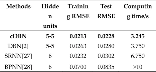
183
the feed forward network. Mean work used in the test set by activating all of the hidden units and
184
attenuate their weights with a certain proportion. This method acts well in some cases. However,
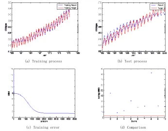
185
since it is used in fine tuning, it needs to be modified before being applied in cDBN.
186
Since values in cDBN’s units are all continuous and over fitting is still a serious problem in
187
unsupervised training, so an improved unsupervised training process with dropout is proposed in
188
this paper. The formula of dropout can be described as follows,
189
𝑠 = 𝑠 ∙ 𝑑𝑟𝑜𝑝𝐹
(8)
190
𝑑𝑟𝑜𝑝𝐹 =
1, 𝑛 ≥ 𝑟
0, 𝑛 < 𝑟
(9)
191
where sj is the state of unit j in hidden layer, it will be decided to be constant or be turned to 0 in one
192
case by dropF, which is dropout fraction as be calculated in (9). n is a random value between [0, 1],
193
and 𝒓𝒅𝒓 means how many percentages of units in a layer will be turned to 0. In the procedure of CD,
194
dropout is supposed to be applied in the processes of calculating sj0 and si0, because these two states
195
affect the next two states in CD, an all of the weights will be recalculated according to sj0 and sj0. And
196
it should be noticed that in some time series forecasting tasks, there are not too many units in the first
197
visible layer, and one of them is supposed to take the value of output in the last case, in this case only
198
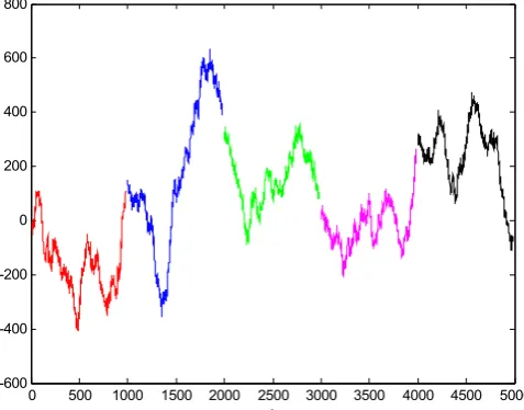
sj0 will perform dropout, otherwise some important information will be lost in the knowledge
199
reconstruction of sj0. When using Contrastive Divergence, the update forms of weights and biases are
200
as follows,
201
∆𝑤 = 𝜂 (< 𝑠 𝑠 > −< 𝑠 𝑠 >)
(10)
202
𝛥𝑏 =
(< 𝑠
> −< 𝑠
>)
(11)
203
𝛥𝑐 =
(< 𝑠
> −< 𝑠
>)
(12)
204
where ηw, ηb, ηc are the learning rate of weight and biases, and <∙> still means what has been
205
addressed above.
206
So,
207
𝑤 (𝑡) = 𝑤 (𝑡 − 1) + ∆𝑤 (𝑡)
(13)
208
𝑏(𝑡) = 𝑏(𝑡 − 1) + ∆𝑏(𝑡)
(14)
209
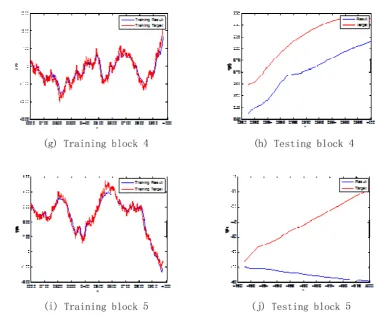
𝑐(𝑡) = 𝑐(𝑡 − 1) + ∆𝑐(𝑡)
(15)
210
where t is the tth epoch been run.
211
Fig.2 shows the schematic diagram of improved dropout in unsupervised learning process,
212
which is the procedure of unsupervised training in a RBM in cDBN. Dashed lines mean that the
neurons are omitted temporally other than permanently, since they will be reactivated in the next
214
epoch. By using improved dropout in unsupervised training, hidden units’ values are turned to be 0
215
randomly according to weights updating rules (8) and (9). This strategy prevents the affection of
co-216
adaptation between some feature detectors since this makes two units in a same layer won’t appear
217
in the same epoch all the time. So the update of weights won’t rely on the interaction of two units,
218
and dropout forces them find more solution spaces and learn knowledge independently and wisely.
219
Dropout can be seen as a kind of mean work, because cDBN with different structures will be activated
220
for each training case, and finally, all of the units will be activated for test set. As regularization is
221
often being used to reduce over fitting, and in fact native Bayes regularization method is a special
222
case of dropout, because native Bayes assumes that the feature detectors are already independent.
223
Native Bayes can learn each feature at a time if training set is small, and still has good results. But
224
improved dropout can learn more than one feature at a time and combine them together at last when
225
all of the detectors are activated, realizing features learning better.
226
0
h ……
1
h
hm0
v
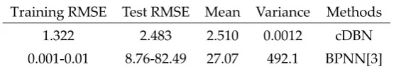
…… nv
Hidden layer1 Visible layer 1v
Weights …… Hidden layer2 RBM Be dropouted unit 0 h …… 1h
hm0
v
…… nv
Hidden layer1 Visible layer 1v
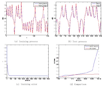
Weights …… Hidden layer2 RBM Be dropouted unit227
Fig 2 Improved Dropout in Unsupervised Learning
228
229
A summarized cDBN training procedure with improved dropout to reduce over fitting is shown
230
as follows.
231
Step 1. Decide how many layers will be included and the size of each layer, and limitation of
232
iteration number.
233
Step 2. Initialize cDBN.
234
Step 3. Put the original data into visible layer which contains m units, and start calculating using
235
formula (4) and (6). By running (8) and (9), the dropout fraction, to get the left units in the epoch, and
236
then perform (5) and (7) which is to calculate the generated data of input, in which procedure,
237
dropout will also be used to omit the units in the first hidden layer.
238
Step 4. Update weights and biases using CD.
239
Step 5. If the stopping condition which has been set in the experiment below is reached, go to
240
step 6. Otherwise go back to step 3.
241
Step 6. If the stopping condition in the last layer is reached, go to step 7. Otherwise, set the output
242
of this RBM be the input of the next one.
243
Step 6. Turn to step 3 and run the next RBM.
244
Step 7. Compare the expected output with the real output to calculate the error. Use back
245
propagation in the process of fine tuning.
246
Step 8. The output of the final output in the last layer is transited to be a unit of the visible layer
247
in the next training case. If this is not the last case, turn to step 3, otherwise, go to step 9.
248
Step 9. Stop running.
249
5. Convergence and stability analysis
250
cDBN can be seen as a probability generation model that contains two hidden layers, as well as
251
a complex model that is made of several simple models. In fact, each pair of neighboring layers of
252
cDBN is a continuous RBM, so the method of unsupervised training can be used in the training
253
process. As a probability generation model which is undirected and based on network energy theory,
continuous RBM uses Contrastive Divergence algorithm’s one step iteration in data pre-train stage
255
to update network weights. Traditional training way transfers the values of hidden and visible units
256
to be Bernoulli value (0 or 1), other than using the probabilities of units themselves. However, in
257
cDBN in this paper, the contradiction theory is avoided by taking the probability to be output by
258
using formulas (6) and (7), so Contrastive Divergence can still be used as a rapid training strategy.
259
Then it will be,
260
𝑠 𝜖[0,1]
(16)
261
𝑠 = 𝜑 ∑ 𝑤 𝑠 + 𝜎 ∙ 𝑁 (0,1)
(17)
262
𝑠 = 𝜑 ∑ 𝑤 𝑠 + 𝜎 ∙ 𝑁 (0,1)
(18)
263
𝑠 = 𝜑 ∑ 𝑤 𝑠 + 𝜎 ∙ 𝑁 (0,1)
(19)
264
The algorithm of CD is to approximate maximum likelihood method, and it is used to learn each
265
weight of continuous RBM in a cDBN. After learning the first RBM, the second one will be stacked
266
on top of the first one, and the output of the first RBM becomes the input layer of the second RBM.
267
By doing this, a multi-layer model is formed. In the procedure of stacking, the input layer of the first
268
continuous RBM is initialled by the original data. When the weights are trained, the output will be
269
copied directly to the input of the second continuous RBM, and then repeat the same training
270
procedure until the termination conditions are reached. So sj1 in equations (16) to (19) is the output
271
of the first RBM (RBM1) as well as the input of the second RBM (RBM2).
272
In the unsupervised learning step, by training one RBM, the algorithm of contrastive divergence
273
(CD) can be seen as a simple version of Markov Chain Monte Carlo (MCMC), so the error after
274
training one RBM may not be 0, but should be close to it. In this part we use ρ to be the error. Then
275
there is,
276
0 < 𝜌 < 1
(20)
277
And there could be several (n) RBMs in a traditional DBN, depending on the tasks. So
278
theoretically, the final error of DBN could be close enough to 0, which is
279
𝜌 ≈ 0
(21)
280
In the process of supervised learning, back propagation will be used, and the training error of a
281
BP network has been researched, which can be 0 according to Weierstrass theory [3]. So the
282
convergence of cDBN will be assured.
283
As a fast training algorithm, CD is in fact not in any approximate function’s gradient decent
284
directions, and as a result, its approximation for maximum likelihood is very rough, so in order to
285
assure this proposed network is capably and stably converging to the solution space and to find the
286
optimal solution, it is necessary to use theory to select hyper parameters through stability analysis
287
for cDBN. And only by analyzing this can the proposed strategy of CD and dropout have the
288
theoretical basis to be used in cDBN. So, by what have been stated above, we’ve got sj1 (RBM1) = si0
289
(RBM2), and according to (16), the output of RBM should be [0,1], so the convergence condition of
290
cDBN is to make sure sj1 ϵ[0,1]. And the theorem of stability is put forward as follows.
291
292
Theorem. When cDBN is stable, sj1∈[0,1], if and only if sj0,si1∈[0,1].
293
Proof. Let sj0∈[tL1,tH1 ], si1∈[tL2,tH2 ], where tL1,tH1 are lower and upper limit of sj0, tL2,tH2 are lower and
294
upper limit of si1.
295
1) Sufficiency:
296
If the middle states of sj0, si1∈[0,1], then when training a RBM using dropout, according to
(17)-297
(19), the output is si1∈[0,1], which is within the prescribed scope. So, cDBN is stable.
2) Necessity:
299
① If cDBN is stable, and if tL1>0. As the transfer function is monotonous, the middle states of sj0, si1,
300
which meet si1> sj0, can be calculated by CD. Hence, tL2> tL1. And according to (19), sj1> si1, which
301
means the output of cDBN is bigger than 0. This contradicts to assumption.
302
② Hence tL1≤0. Similarly, tL1≥0.
303
③ So, tL1=0. By using the same proof, we have tH1.
304
④ Hence sj0∈[0,1].
305
⑤ Similarly, when doing Gibbs sampling using CD, the output is also between [0,1], which means
306
si1ϵ[0,1].
307
Q.E.D.
308
From the proof we know that the process of dropout doesn’t affect the stability of cDBN, and
309
according to the theorem, there is
310
𝑠 = 𝜃 + (𝜃 − 𝜃 ) ∙ 𝑠 = 𝜃 + (𝜃 − 𝜃 ) ∙ (22)
311
will be assured, and this equation is the selecting basis of hyper parameters. If Gaussian noise is set
312
to be 0, for every x>0, we have 0<e-x<1, so sj0 ϵ[(θH+θL)/2, θH]. Then the selection of θL=-1, θH =1, aj=1
313
can make formula (15) workable. In this cDBN, there are only two hidden layers. According to the
314
convergence and stability analysis, no matter how many RBMs are stacked in a cDBN, if the input
315
and output of cDBN are [0, 1], the intermediate state of learning must be continuous values in [0, 1].
316
It makes sure that the network is stable and reliable in training process.
317
6. Experiments and Analyses
318
Time series forecasting is one of the most common and important tasks in real world. It uses
319
statistics and analysing methods on historical data, learns the inherent law and trend, then predicts
320
the possible value of the future data before providing decisions for industries. Because the sensitive
321
features of inner and outer environment, modelling and predicting for time series data is a complex
322
nonlinear problem, which is important and challenging. Traditional methods, such as linear
323
processing and least square, process the input data in a special way before using, and usually
324
resulting in bad predictions, and thus they are not suitable to solve these tasks. cDBN trains data in
325
an unsupervised way and has very powerful feature learning and extracting function. Besides,
326
according to Weierstrass’s first theorem, Neural Networks (NNs), as a data-driven model, can
327
approximate any nonlinear functions in any accuracy. In additionally, cDBN can be seen as a
black-328
box model in the training process. So in order to test the short term and long term predicting abilities,
329
cDBN is put forward in some experiments below. The input of cDBN is the real data of time series,
330
and in the experiment of long term prediction, the last predicted data will be set as one of the input
331
unit in the next step of prediction. Although there is still lack of good algorithms for deciding the size
332
of each hidden layer and empirical has to be implied here, improved dropout has the ability of
333
reducing over fitting. Different layer sizes can be tried, and the larger one can be chosen if multi-tasks
334
are presented. Last but not least, only one output neuron is used in cDBN which equals to the
335
predicted number.
336
Four experiment belonging to computational simulation and real-world application are
337
explored in this section. First, the simulation experiments of Lorenz chaos series prediction will be
338
conducted. Second, a long-term prediction called CATS Benchmark missed data prediction will be
utilized to testify the model. Once the model has been proved effective, two real-world applications
340
will be introduced in experiments three and four. In the first real-world application, the technic of
341
unsupervised dropout will also be tested, and the performance variance with right to different
342
dropout rates will be analysed.
343
6.1 Simulation Experiment 1: Lorenz chaos series prediction
344
The experimental target is to check whether the proposed cDBN is capable of predicting short
345
term data accurately with a simplified structure, whether the improved dropout can further improve
346
the accuracy. Chaotic time series forecasting is a typical benchmark problem on testing new methods
347
of neural networks, and since Lorenz effect indicates the sensitive dependence on initial conditions
348
of chaos, is barely feasible to forecast long term data in this task. However, short-term prediction such
349
as one-ahead prediction can be realized if a predictor approximates the nonlinear system enough.
350
The Lorenz chaos equations are as follows,
351
⎩ ⎪ ⎨ ⎪
⎧ = 𝜎(𝑦 − 𝑥 ) = −𝑥 𝑧 + 𝛾(𝑥 − 𝑦 )
= 𝑥 𝑦 − 𝛽𝑧
(23)
352
where x is convection intensity, y indicates horizontal temperature difference between rising airflow
353
and sinking airflow, while z is vertical temperature difference between them. The parameters are
354
σ=10, γ=28, β=8/3.
355
In the experiment, time series data on dimension x is processed. In the generated series, the first
356
1,000 sets are omitted to reduce affection of initial state on the series. The training set has 1,500 values,
357
and test set is the following 1,000 numbers. Three nodes in input layer are introduced to do one step
358
prediction, that is to say, values at time (t-2), (t-1), t are set to be input, and the output is value at the
359
next time t+1. RMSE is introduced as the evaluation index,
360
𝑅𝑀𝑆𝐸 = ∑ ( ( ) ( )) (24)
361
where y(k) and ỹ(k) indicate the ideal output and observed output at time k respectively. In order to
362
verify improved dropout’s effectiveness, different kinds of structures will be tried from 10-10 to
100-363
100, and the improvement will be recorded. Epochs in the stagy of automatic knowledge learning
364
(unsupervised learning) is 100 and fine tuning (supervised learning) learning rate is 2. Dropout
365
fraction in unsupervised learning is 0.2, which means 20% of the hidden units will be set to 0
366
randomly in training process. Fine tuning iterations are set as 5,000. The results are shown in Table 1
367
and Fig 3.
368
Table 1 Results of Lorenz experiment
369
Methods Hidde
n units
Trainin
g RMSE
Test
RMSE
Computin
g time/s
cDBN 5-5 0.0213 0.0228 3.245
DBN[2] 5-5 0.0263 0.0280 3.750
SRNN[27] 6 0.0232 0.0302 6.750
370
Fig 3 Results of Lorenz experiment
371
372
From Fig.3 (a) and (b), it can be seen that even though it is hard to learn the knowledge at some
373
of the sharp places, cDBN is still capable of realizing rapidly learning and tracking the function line
374
well. With the structure of 3-5-5-1, cDBN with dropout is trained with the training error 0.0213. And
375
in testing stagy, the network responds somehow at the same quality, it presents very good
376
approximate ability and generalization ability. Also, the test RMSE is reduced to 0.0228, better than
377
DBN without dropout and some other methods. BPNN is the most classical model in solving the
378
problem, but both the training and test error are big. And SRNN is one outstanding method that is
379
proposed in [27], by using which the test error is a little bigger than using DBN, the training error is
380
smaller. But when applying the proposed network in this paper, we’ve had both very small training
381
and test error in the experiment. In fact, the time consuming is a little less because the computing
382
speed is more depend on contrastive divergence than other factors, and sometimes it’s a little faster
383
due to the time saving by not computing a part of the neurons.
384
Fig.3 (c) shows the error decreasing line in fine tuning, from which we can see that the
385
convergence speed is quite rapid thus it saves computing time. That is because the weights have been
386
initialized by unsupervised training are already in a good solution area. Fig 3(d) presents the
387
comparison of cDBN that has the same structure both with and without dropout. The red line shows
388
test RMSE of cDBN with dropout while the blue one is without. From Fig 3(d) we can see when the
389
hidden units are 3-3, cDBN without dropout acts better, that is because when the size of the layer is
390
small, features in each of them are too important to be ignored. Then, when more units are added,
391
over fitting becomes a problem so the test RMSE increases. However, cDBN with dropout improves
392
the learning effectiveness by preventing co-adaptation of feature detectors, and test RMSE can be
393
kept at a low level.
Besides, when the hidden units are the same, cDBN with dropout strategy basically responds
395
better than some other methods. This is because cDBN uses the second hidden layer to extract more
396
features from the first hidden layer, and is capable of learning a better distributed presentation of
397
input.
398
6.2 Simulation Experiment 2: CATS Benchmark missed data prediction
399
The second experiment is to verify whether cDBN is capable of predicting long term data
400
accurately, and neurons respond better than those without dropout. The used database is
401
Competition on Artificial Time Series (CATS benchmark), which was brought up in [29] and later
402
became a common benchmark to test new models in AI. This benchmark consists of 5 data blocks,
403
each of which has 1,000 sets of data, the first 980 are given and the rest 20 are missed, see in Fig 4.
404
405
Fig 4 CATS benchmark Data
406
407
So in all the 5 blocks, 100 sets in total are needed to be predicted, and then the results can be
408
compared by E1 and E2.
409
𝐸1 =∑ ( ( ) ( )) +∑ ( ( ) ( )) +∑ ( ( ) ( )) +∑ ( ( ) ( )) +∑ ( ( ) ( )) (25)
410
𝐸2 =∑ ( ( ) ( )) +∑ ( ( ) ( )) +∑ ( ( ) ( )) +∑ ( ( ) ( )) (26)
411
Although the line is quite sharp, the data in CATS still has certain internal laws, and finding
412
them is the task for DBN before predicting missed data. For each of the first 4 missed blocks, both the
413
information before and after the missed block can be used in the training process to learn as much
414
knowledge as it can. But for the last missed block, no later information is given, so only the data
415
before can be used. As a result, mission E1 is harder than E2, because E1 has to concern all of the five
416
missed blocks while E2 only has to concern the first four.
417
As there are 20 numbers in each missed block, it’s a long term prediction task. The input nodes
418
are set to be 10, and in the testing process, the last case’s prediction, x(t), will become one of the input
419
node in the next prediction for x(t+1). In order to train the training set and to verify dropout’s
420
effectiveness, and to make the comparison easier, a fixed structure of 10-20-40-1 will be chosen.
421
0 500 1000 1500 2000 2500 3000 3500 4000 4500 5000 -600
-400 -200 0 200 400 600 800
For each missed block, the sets before and after it are trained at once. The epochs in knowledge
422
learning process are 200, dropout fraction is 0.5, which means half of the hidden units are dismissed
423
in each epoch, but they will return in the next epoch. Learning rate in fine tuning is between 0.5 and
424
1, fine tuning iterations are set as 5,000. Results can be found in Fig 5. The results indicate that for
425
each block, cDBN using improved dropout attains a very good learning result and reaches to a
426
satisfied prediction. The original line of CATS is extremely sharp especially in short term, since there
427
are many obvious ups and downs in it. The learning line of cDBN is relatively smooth, which means
428
it has good generalization ability for the missed numbers.
429
430
431
433
434
Fig 5 CATS benchmark experimental results of cDBN using improved dropout
435
436
Fig 5(b) and (f) indicate the prediction for the first and the third block, from which we can see
437
the testing lines are very close to the original ones. Fig 5(d) and (h) are the testing lines of missed
438
block 2 and 4, and they are somehow parallel lines which show the network has learnt enough
439
knowledge in predicting and the result line has the same trend with an error of around 20. Fig 5(j)
440
indicates the prediction on block 5, and it can be seen the network is hard to make a good prediction
441
and the trend is wrong. This result meets what have been discussed above.
442
Table 2 Comparison between different models in CATS benchmark
443
E1 Model E2 Model
459.151 cDBN 215.611 cDBN 408 Kalman
Smoother[30]
222 Ensemble
Models[31] 771.455 DBN[18] 618.912 DBN[18]
1215 PSO-DBN[20] 979 PSO-DBN[20]
Table 2 compares the results with some different other models. Kalman Smoother and Ensemble
444
Models in the second row got the first place in IJCNN04’s competition. When using cDBN without
445
dropout, we’ve had E1 = 771.455, E2 = 618.912 worse than the both two models but better than the
446
others such as Hierarchical Bayesian Learning and MLP. And if the dropout fraction is set as 0.5, the
447
test errors are reduced to E1 = 459.151, E2=459.151 which is a big step forward than the one without
448
dropout in row 4.
449
The CATS benchmark experiment shows that cDBN is capable of predicting long term data
450
accurately and the strategy of dropout makes the prediction better by overcoming over fitting
problem. Although this model cannot select network size such as how many layers would be the best,
452
the strategy of improved dropout helps to improve the learning effectiveness by changing network
453
structure randomly in the unsupervised training process, thus it can also be seen as a structure
self-454
organizing model. And if more structures are implied, more accuracy results may be realized.
455
6.3 Real-world application 1: CO2 forecasting
456
The experiment of this part is to verify whether cDBN with dropout can be used in real world
457
applications that contain noise, and whether the convergence is stable. cDBN transfers the results of
458
pre-training in deep belief network to the initial weights in the next neural network, and then uses
459
back propagation algorithm to do fine tuning. This training method is quite valuable especially in
460
those tasks whose training set is small, this is because, as a matter of fact, initial weights can have a
461
significant affection on the final models that are trained, and the weights that have been pre-trained
462
are nearer to the optimal weights in solution space than those that have not. However, over fitting
463
will be another serious problem in this condition since the weights are easy to be over trained.
464
Environmental issue has been one of the most concerned themes of the world. CO2 concentration
465
change is caused by many factors, such as geographical factors, human social activities, marine
466
monsoon and so on. Human society is affected significantly due to CO2 change. For instance, when
467
density of CO2 is too high, greenhouse effect can be a furious problem in metabolism. As a result of
468
this, forecasting CO2’s density is not only meaningful for scientific investigation, but also provides
469
reference for local government and factories to control CO2 emission. 2.529,
470
Because of the errors caused by external factors, sampling CO2’s density in short term can barely
471
reflect local CO2’s change, as a result, studying on long term CO2’s density after being de-noised is
472
necessary. In order to assure the accuracy of the sampled data, CO2 data that is used to forecast the
473
global climate change should be sampled in those reigns that haven’t been polluted by urban
474
discharges.
475
(a) Training process (b) Test process
(c) Training error (d) Comparison
476
Fig 6 Experimental result of CO2 forecasting
In this experiment, the data of Mauna Loa, Hawaii 2,220 sets in total from 1965 to 2000 is used
478
[32]. Training set is 1,220 sets and the following 1,000 are left for testing. Also, in order to test
479
improved dropout, different kinds of structures will be attempted from 10-10 to 50-50, and the
480
improvement will also be recorded. Epochs in the step of knowledge automatic learning are 100 and
481
dropout fraction is 0.5. Learning rate in fine tuning (supervised learning) is set to be 3 and the
482
iterations are 5,000. The result with 40-40 neurons is shown in Fig 6.
483
Fig 6(a) is the training process while (b) shows the test process, and (c) represents the training
484
error in fine tuning. It can be seen from (a) that the density of CO2 changes regularly according to
485
seasons, and has a trend of rising year by year. cDBN is capable of de-noising in this experiment, and
486
the training and testing results turn out to be good.
487
In the features-learning stagy, the network acts bad at first but it manages to find the inter rules
488
rapidly. And in the generalization stagy, the network responds accurately in the beginning and
489
finally fails to forecasting, this may be because the features of human activities at the end of last
490
century have not been learnt well enough.
491
Table 3 Result data of CO2 forecasting
492
Training RMSE Test RMSE Mean Variance Methods
1.322 2.483 2.510 0.0012 cDBN
0.001-0.01 8.76-82.49 27.07 492.1 BPNN[3]
Table 3 is associated with Fig6(d), which represents the results of using cDBN and BPNN, and
493
it is easy to be seen that cDBN is better in most places. By running each program 10 times, training
494
errors in BPNN are quite small, which are around 0.001-0.01, which shows a good chance to be over
495
fitting. The tests RMSE are 9.7852, 44.6642, 8.7591, 12.3830, 31.0149, 18.8894, 20.8709, 82.4998, 21.5635,
496
and 20.2909. The mean value is 27.0721, and the variance is 492.1079. While tests RMSE of improved
497
cDBN the test RMSE are 2.483, 2.495, 2.519, 2.529, 2.491, 2.500, 2.601, 2.489, 2.492, 2.500. The mean
498
value is 2.510 and variance is 0.0012, which means it can almost always convergent to the optimal.
499
Table 4 and Figure 7 records the improvements of cDBN with different dropout rates. When the
500
hidden units are set to be 10-10, cDBN without dropout acts better, that is probably because when
501
the units are few and no need to concern about over fitting, and features in each of them are too
502
important to be omitted. When putting more nodes in hidden layers, the base test RMSE will raise,
503
but dropout improves the learning effectiveness by preventing co-adaptation of feature detectors,
504
keeping test RMSE at a low level. And in different conditions, different degrees of improvement have
505
been achieved. For example, with the structures of 20-20, 30-30 and 50-50, the decrease of errors from
506
4.43% to 65% can be achieved, and when the hidden units are 40-40, the error can be decreased by as
507
much as 69.55%. It can also be observed that the final error obtained by the model is sensitive to the
508
choice of dropout fraction. The best performance will be achieved when structure is 40-40 with
509
dropout rate 0.5, which is very close to using a structure of 20-20 directly, as a result, this method can
510
also provide a way of find the best structure with high stability in real-world application. This
511
experiment also finds that a lager structure with dropout rate 0.5 is easier to achieve higher prediction
512
accuracy.
514
Fig 7 Improvements of different dropout rates
515
516
Table 4 Comparison of different dropout rates
517
Structures Dropout Training RMSE
Test RMSE
Improve ment
10-10
0 1.383 2.887
0.2 1.166 4.509 -56.18%
0.5 1.101 6.079 -110.56%
0.8 1.084 6.123 -112.09%
20-20
0 1.355 2.733
0.2 1.292 2.750 -0.62%
0.5 1.315 2.612 4.43%
0.8 1.312 2.719 0.51%
30-30
0 0.933 7.781
0.2 1.261 2.720 65.04%
0.5 1.244 3.018 61.21%
0.8 1.256 2.857 63.28%
40-40
0 0.935 8.155
0.2 0.884 9.689 -18.81%
0.5 1.322 2.483 69.55%
0.8 1.370 2.533 68.94%
50-50
0 2.163 7.124
0.2 0.950 9.045 -26.97%
0.5 1.375 2.530 64.49%
0.8 1.418 2.756 61.31%
6.4 Real-world application 2: Wastewater parameter prediction
518
In this experiment, cDBN will be applied to another real-world application, wastewater
519
parameter prediction. In recent decades, wastewater problem has become one of the major
environmental concerns. Wastewater treatment process (WWTP) is a highly nonlinear dynamic
521
process. In order to minimize microbial risk and optimize the treatment operation, many variables
522
must be obtained real-timely, in which, biochemical oxygen demand (BOD), chemical oxygen
523
demand (COD), suspended solid (SS),PH level and nutrient levels, total nitrogen (TN)-containing,
524
total phosphorus (TP)-containing are the most important ones. Subject to large disturbances, where
525
different physical (such as settling) and biological phenomena are taking place. It is especially
526
difficult to measure many parameters of WWTP online. Although wastewater quality parameters can
527
be measured by laboratory analysis, a significant time delay, which may range from a matter of
528
minutes to a few days, is usually unavoidable. This limits the effectiveness of operation of effluent
529
quality. Thus, a water quality prediction model is highly desirable for wastewater treatment.
530
The data used here is from the water quality testing daily sheet of a small-sized wastewater
531
treatment plant in Beijing, China. The data has 867 sets and it includes information on influent BOD,
532
influent SS, influent NH4-N, influent TP, PH. Only the five mentioned here were used to predict the
533
effluent COD and SS. The proposed network is implemented to model wastewater treatment process
534
with the inputs being the value of the above specified five variables, and the outputs being the
535
effluent COD and SS. The challenges of this experiment are twofold. Frist, instead of predicting one
536
parameter, this is a multi-parameter problem, and each parameter may have intern affection on each
537
other. Second, the data collected is from a small-sized plant, it is not many, and may contain large
538
amount noise. Results are shown in Figure 8 and Table 5.
539
Figure 8 (a) and (b) are testing results on predicting COD and SS, (c) is the trend of mean squared
540
error in training, and (d) shows the regression. Table 5 records testing RMSE on COD and SS using
541
different dropout rates. This experiment proves that cDBN is capable of predicting correctly on a
542
multi-parameter problem. Normally it can convergent in 200 supervised learning steps with high
543
regression rate. This experiment also proves that network structure and dropout rate still have
544
impressive affects on the test RMSE. Low testing RMSE on COD can be observed where structure is
545
large and dropout rate is small, while low SS testing RMSE can be find where structure is not too
546
large and dropout rate not too big. This is probably because the dataset used is small, and predicting
547
COD is much more complicated than SS, so COD needs a larger structure and more hidden neurons
548
to learn the input features.
Time
0 50 100 150 200 250 300 10
15 20 25 30 35 40 45 50
Ideal Output Prediction
Time
0 50 100 150 200 250 300 0
5 10 15 20 25 30 35 40 45 50
Ideal Output Prediction
448 Epochs
0 50 100 150 200 250 300 350 400 10-5
10-4
10-3
10-2
10-1
100 Best Training Performance is 0.0061117 at epoch 4 Train Best Goal
Target
0 0.2 0.4 0.6 0.8 1 0
0.1 0.2 0.3 0.4 0.5 0.6 0.7 0.8 0.9
1 Training: R=0.94149 Data
Fit Y = T
550
Fig 8 Experimental result of Waste Water Parameter Prediction
551
552
Table 5 Testing RMSE using different dropout rates
553
Structures Dropout Test
RMSE/COD
Test RMSE/SS
6-6
0 6.917 6.353
0.2 7.645 5.561
0.5 7.911 4.995
0.8 7.274 6.507
10-10
0 7.818 4.438
0.2 6.402 3.960
0.5 6.605 6.695
0.8 8.329 3.719
20-20
0 5.403 5.100
0.2 6.372 6.614
0.5 8.213 8.341
0.8 8.159 5.153
7 Conclusion
554
cDBN is a kind of deep learning neural network that has transferred values in hidden and visible
555
layers from discrete to continuous. The main work of this study is: 1) A Continuous DBN with two
556
hidden layers is proposed, in which an improved dropout strategy for unsupervised learning is
implemented. Besides, Contrastive Divergence is introduced to raise the convergence speed. 2) A
558
stability theorem is brought up and proved. By analysing network’s convergence and stability, the
559
hyper-parameters are given. 3) The experiments of Lorenz time series forecasting, CATS benchmark
560
prediction, CO2 forecasting and wastewater parameter prediction are implemented and have verified
561
that the proposed network is capable of learning information features wisely and has good
562
generalization ability. Besides, results show simplified structure, high accuracy and effective
563
convergence. The experiments have also implied that cDBN can not only be used in benchmark tasks,
564
but also can solve real world applications in industries.
565
Future works will focus on the two points. 1) In the aspect of algorithm, more useful structure
566
self-organizing methods could be studied and improved in cDBN to attain better approximate ability.
567
By increasing and omitting nodes more intelligently, cDBN could reach an improved state for one
568
task. 2) In the aspect of real-world applications, the effectiveness of cDBN in other fields could be
569
studied, for instance in intelligent control and regression problems.
570
Acknowledgements and Funding
571
This work is supported by the National Science Foundation of China under Grants 51711012 and
572
51477011, and Beijing Municipal Education Commission under Grants KM201811232016.
573
Author Contributions: methodology, Q.C, G.P.; software, G.P.; validation, Q.C; writing—original
574
draft preparation, G.P; writing—review and editing, M.Y.; supervision, J.W.; project administration,
575
J.W; funding acquisition,Q.C.
576
Conflicts of Interest: The authors declare no conflict of interest.
577
References
578
[1] Hinton, G., Salakhutdinov, R.: 'Reducing the dimensionality of data with neural networks',
579
Science, 2006, 313, (5786), pp. 504-507
580
[2] Hinton, G., Osindero, S., The, Y.: 'A fast learning algorithm for deep belief nets', Neural
581
Computation, 2006, 18, pp. 1527-1554
582
[3] Rumelhart, D., Hinton, G., Williams, R.: 'Learning representation by back-propagating errors',
583
Nature, 1986, 232, pp. 533-536
584
[4] Bengio, Y., Olivier, D.: 'On the expressive power of deep architectures', Algorithmic Learning
585
Theory, Springer Berlin Heidelberg, 2011, 18-36
586
[5] Bengio, Y., Pascal, L., Dan, P., Hugo, L.: 'Greedy Layer-Wise Training of Deep Networks',
587
Advances in Neural Information Processing Systems 19 (NIPS 2006), MIT Press, 2007, pp. 153-160
588
[6] Bengio, Y.: 'Learning Deep Architectures for AI', Foundations & Trends in Machine Learning,
589
2009, 2, (1), pp. 1-127
590
[7] Deselaers, T., Hasan, S., Bender, O.: 'A deep learning approach to machine transliteration', Proc of
591
the 4th Workshop on Statistical Machine Translation, 2009, pp. 233-241
592
[8] Dahl, G., Dong, Y., Deng, L.: 'Large vocabulary continuous speech recognition with
context-593
dependent DBN-HMMS', Proc of IEEE International Conference on Acoustics, Speech and Signal
594
Processing, 2011, pp. 4688-4691
595
[9] Itamar, A., Derek, C., Rose, T.: 'Deep Machine Learning-A New Frontier in Artificial Intelligence
596
Research', IEEE Computational Intelligence Magazine, 2010, 11: 13-18
597
[10] LeRoux, N., Bengio, Y.: 'Representational power of restricted boltzmann machines and deep
598
belief networks', Neural Computation, 2008, 20, (6), pp. 1631-1649
[11] Taylor, G., Hinton, G., Roweis, S.: 'Modeling Human Motion Using Binary Latent Variables',
600
Advances in Neural Information Processing Systems 19, Proceedings of the 2006 Conference, 2006,
601
pp. 1345-1352
602
[12] Mohamed, A., Dahl, G., Hinton, G.: 'Acoustic modeling using deep belief networks', IEEE
603
Transactions on Audio, Speech and Language Processing, 2012, 20, (1), pp. 14-22
604
[13] Jurgen, S.: 'Deep Learning in Neural Networks: An Overview', Technical Report IDSIA-03-14,
605
2014, pp. 1-88
606
[14] Langkvist, M., Karlsso, L., Loutfi, A.: 'A review of unsupervised feature learning and deep
607
learning for time-series modeling', Pattern Recognition Letters, 2014, 42, (6), pp. 11-24
608
[15] Hinton, G., Osindero, S., Welling, M., et al.: 'Unsupervised Discovery of Nonlinear Structure
609
Using Contrastive Backpropagation', Cognitive Science, 2006, 30, (4), pp. 725-731
610
[16] Chen, H., Murray, A.: 'A continuous restricted boltzmann machine with an implementable
611
training algorithm', IEEE Proc Vision Image Signal Process, 2003, 3, (150), pp. 153-158
612
[17] Ren, Z., Shen, F., Zhao, J.: 'A Model with Fuzzy Granulation and Deep Belief Networks for
613
Exchange Rate Forecasting', IJCNN2014, Beijing, 2014, pp. 366-373
614
[18] Hinton, G., Srivastava, N., Krizhevsky, A.: 'Improving neural networks by preventing
co-615
adaptation of feature detectors', arXiv preprint arXiv:1207.0580, 2012
616
[19] Längkvist, M., Karlsson, L., Loutfi, A.: 'A review of unsupervised feature learning and deep
617
learning for time-series modeling', Pattern Recognition Letters, 2014. 42, (6), pp. 11-24
618
[20] Kuremoto, T., Kimura, S., Kobayashi, K.: 'Time series forecasting using a deep belief network
619
with restricted Boltzmann machines', Neurocomputing, 2014, 137, pp. 47-56
620
[21] Bergstra, J., Bardenet, R., Bengio, Y., et al.: 'Algorithms for hyper-parameter optimization', Nips,
621
2011, 24, pp. 2546-2554
622
[22] Bergstra, J., Bengio, Y., Bottou, L.: 'Random search for hyper-parameter optimization', Journal of
623
Machine Learning Research, 2012, 13, (1), pp. 281-305
624
[23] Chao, J., Shen, F., Zhao, J.: 'Forecasting Exchange Rate with Deep Belief Networks', IJCNN11,
625
2011, PP. 1259-1266
626
[24] Chen, J., Jin, Q., Chao, J.: 'Design of Deep Belief Networks for Short-Term Prediction of Drought
627
Index Using Data in the Huaihe River Basin', Mathematical Problems in Engineering, 2012, PP. 1-16
628
[25] Hinton, G.: 'Training Products of Experts by Minimizing Contrastive Divergence', Neural
629
Computation, 2002, 14, pp. 1771-1800
630
[26] Zhang, S., Bao, Y., Zhou, P., et al.: 'Improving deep neural networks for LVCSR using dropout
631
and shrinking structure', 2014 IEEE International Conference on Acoustics, Speech and Signal
632
Processing (ICASSP), 2014, PP. 6849-6853
633
[27] Chen, Q., Chai, W., Qiao, J.: 'A Stable Online Self-Constructing Recurrent Neural Network',
634
Lecture Notes in Computer Science, 2011, 6677, pp. 122-131
635
[28] Li, C., Pin, C., Chang, F.: 'Reinforced Two-Step-Ahead Weight Adjustment Technique for Online
636
Training of Recurrent Neural Networks', IEEE Transactions on Neural Networks and Learning
637
Systems, 2012, 23, pp. 1269-1278
638
[29] Amaury, L., Erkki, Q., Olli, S.: 'Time Series Prediction Competition: The CATS Benchmark',
639
IJCNN04, Budapest, 2004, pp. 1615-1620
640
[30] Sarkka, S., Vehtari, A., Lampinen, J.: 'Time Series Prediction by Kalman Smoother with Cross
641
Validated Noise Density', IJCNN04, Budapest, 2004, 2, pp. 1653-1657
[31] Wichard, J., Ogorzalek, M.: 'Time Series Prediction with Ensemble Models', IJCNN04, Budapest,
643
2004, pp. 1625-1629
644
[32] CO2Now.org. (2015). [Online]. Available: http://co2now.org/
645
[33] Chang X, Yu Y L, Yang Y. Semantic Pooling for Complex Event Analysis in Untrimmed Videos.
646
IEEE Transactions on Pattern Analysis & Machine Intelligence, 2017, 39(8):1617-1632.
647
[34] Mnih V, Badia A P, Mirza M. Asynchronous Methods for Deep Reinforcement Learning.
648
Proceedings of the 33rd International Conference on Machine Learning, New York, NY, USA, 2016.
649
[35] Qiao J, Pan G, Han H. A regularization-reinforced DBN for digital recognition. Natural
650
Computing, 2017, 2:1-13.
651
[36] Pan G, Fu L, Thakali L. Development of a global road safety performance function using deep
652
neural networks. International Journal of Transportation Science & Technology, 2017, 6(3), 159-173.
653
[37] G Pan, L Fu, L Thakali, M Muresan, M Yu. An Improved Deep Belief Network Model for Road
654
Safety Analyses. 2017, TRB 2018 (Accepted).