Estimating the Beginning and End Dates of Covid-19 for several countries using the Logistic Model

Estimating the Beginning and End Dates of

Covid-19 for several countries using the

Logistic Model

Ademir Xavier Jr.

Brazilian Space Agency, Brasilia/DF, Brazil.

April 17, 2020

Abstract

This note applies the Logistic model approximation to determine the suitable start and end dates for the observed epidemic curves in the total number of cases for different countries. The Logistic model is presented and explicit relations for the beginning and end dates are obtained together with the total epidemic duration. Using data from Brazil, Germany, Italy, and South Korea, the extreme dates are calculated. Since the epidemic onset time is found, a fair comparison of the epidemic curve for these countries is obtained. The result does not depend on the poor statistics available in the early phase of the epidemic when the initial number of infectives is unknown. In fact, the total duration depends only on the characteristic time parameter of the LM model.

Keywords: covid-19, forecast, epidemic, logistic model, pandemic.

1 Introduction

The current Covid-19 epidemics is a new challenge to the public health au-thorities and a threat to the world. The outbreak should be correctly man-aged as a task that starts by acquiring accurate information about its begin-ning date. The end date is much harder to predict since it is the result of

*_{E-mail: [email protected]}

a complex chain of actions and interactions between the population and the disease. The effect of quarantine, testing policy, and vaccination impacts the future circulation of the virus.

Such a challenge calls for the use of models and simulation work in order to access much-hidden information beyond publicly available data. As it is well known, the so-called Logistic model (LM) [3] can capture the general evolution of many epidemics, having been widely observed in Nature. It leads to accurate descriptions of closed populations in the limit of large numbers since it is the solution of a deterministic model [1, 2, 3].

In this work, the evolution of the LM is used as an approximation to estimate the extreme dates of the epidemic. The beginning date is hard to estimate because the number of initial infectives introduced in the host population is unknown and the first cases are generally poorly notified. On the other hand, the end date is also difficult to determine for the reasons outlined above. This note applies the Logistic model by least-square fitting of the LM as described previously[4] and then calculating the dates as a byproduct of data fitting using the publicly reported number of cases.

2 The Logistic Model

Given a closed population with N individuals at a given time t, the rate of change of the population size can be modelled by the differential model

dN dt =rN

1− N

K

, (1)

withrthe rate of population growth andKthe so-called “carrying capacity”[3]. When N is small, the population growth is approximately proportional to

rN. Ast → ∞, the population size tends to K and the growth stops. Eq. 1 has as solution

N(t) = K

1 +Ae−rt. (2)

withAa factor associated with the initial population size. The growth factor

Given Eq.1, the growth rate is written explicitly in term of the time as

˙

N = dN

dt =

rAKe−rt

(1 +Ae−rt₎2. (3)

From this equation it is possible to see that, fort →0, the LM is in fact an exponential law

N = Ke

rt

A+ert ≈ K

Ae rt

, (4)

from which it is possible to relate A and K to the initial population number

N(0). Therefore, in the early phase, the growth is simply given by≈N(0)ert_.

On the other hand, as t → ∞, N(t)→ K, and the carrying capacity is the final population size.

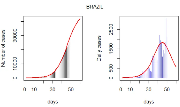
As described in [4], the model should be applied with care to describe the evolution of epidemics like Covid-19 since, in general, the reported number of infections is a compilation of cases from several regions which distinct epi-demic starting dates. Using Brazil as an example, the reported case curve is a sum of the contribution from widely separated cities with different popula-tions and starting dates and subjected to a variety of errors. However, within certain limits, since the growth is dominated by large cities (as S˜ao Paulo and Rio de Janeiro) where the epidemics started almost simultaneously, the observed curve of reported cases seems to be fairly well described by the function of Eq. 1, see Fig.1.

The “maximum epidemic time” ¯t is estimated as the time when the max-imal daily rate occurs. Since

d2_N

dt2 =

r2_AKe−rt

(1 +Ae−rt₎2

2Ae−rt

(1 +Ae−rt₎−1

, (5)

the condition d2N/dt2 = 0 leads to

¯

t= lnA

r , (6)

and ˙N is maximum. At this time, N(¯t) = K/2 and

˙

N(¯t) = Kr

4 . (7)

Figure 1: Evolution of reported Covid-19 cases in Brazil (left) and daily num-ber of cases (right) with data from February 27-th to April 16-th, 2020. The red line is the LM model adjusted with K=46105, r =0.1586 and A=1311. Data set available at [5].

3 Finding the beginning and end dates

While it is possible to define an initial time for the epidemic onset (for ex-ample, by finding the date of the first reported case), the evolution given by Eq. 1 never ends. Therefore, we use Eq. 2 as an indicator for the beginning and end dates since it falls off as t → ∞. Let α be a positive real number with α 1. Define the function

f(t) = ˙

N(t)

N(¯t), (8)

the extreme dates are found by

α=f(t), (9)

number of cases is a fractionαof the observed maximum given by Eq.7. The start date is when the value of f(t) exceeds the fraction while the end occurs when it is just below α.

By setting x= exp(−rt), Eq. 9 leads to

A2x2+ 2A

1− 2

α

x+ 1 = 0, (10)

with the discriminant ∆ = 4A√1−α/α and two solutions:

x±=

(2−α)±2√1−α

αA . (11)

Now, for 0 < α1,

√

1−α≈1− 1 2α−

1 8α

2_,

and approximate values for the times are found from

x+≈

4−2α αA , x−≈

α

4A

(12)

The total number of cases for each solution is

N(x+)≈

Kα

4−α,

N(x−)≈ K 1 +α/4.

(13)

Therefore, t+ = t0 and t− = t∞ with t =−ln(x)/r. Defining ∆t =t∞−t0

as the total duration of the epidemics, it is possible to show for α1 that

∆t≈ 1

rln

4(4−2α)

α2

, (14)

Parameter S. Korea Brazil Italy Germany ¯

t Mar-2 Apr-11 Apr-27 Apr-9

t0 Jan-31 Feb-29 Feb-10 Feb-26

t∞ Apr-3 May-23 May-11 May-23

∆t (days) 63 84 91 87

K 10614 46105 179766 271899

A 7734 1311 228 9665

r 0.2140 0.1586 0.1460 0.1438

τ (days) 4.7 6.3 6.8 6.5

Table 1: Extreme dates, time of maximum and other parameters of the LM model for several countries for α=0.5% and data compiled on April 16-th. The original data used to calculate these values can be found on the HDE website [5].

4 Application

In fact, the value ofr varies for different populations and is strongly affected by the error in the validity assumption of the LM model to describe the evolution of Covid-19 using the public number of cases. For the example shown in Fig. 1, τ = 6.3 days, which represents an average growth rate fitted using all data available on the date (April 16-th, 2020). If n is the observation date (for which a set of data points from 1 to n is available), the fitting procedure described in [4] produces a sequence {K(n), A(n), r(n)} and, therefore t0(n) and t∞(n), which evolves withn.

By the time of this writing, using the total number of cases for Brazil with data available until April 16-th (n = 49, Fig.1), the sequence t0 = {3,2,4,4,3,4,5} and t∞ ={87,86,83,83,84,83,79} was obtained when the least-square fit was run backwards in time for n ={49,48,47,46,45,44,43}. The value of αis 0.5%. A fixed time window with m= 12 is used (the value of m is defined in [4]). The date n = 1 corresponds to February 27th while

n = 85 is May 21st. Thus a total duration ≈ 80 days is predicted for Brazil with an epidemic end time by the end of May. Since the daily maximum according to Eq. 8 is ˙Nmax ≈ 1900 cases per day, the epidemic threshold for

the daily cases in Brazil given α is ≈10.

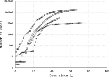
have total predicted periods in the range of 84-90 days. Therefore, the value of τ is nearly the same (≈ 6.5 days). The only country for which the value of K has converged is South Korea. The other ones may change with time. The predicted final dates ate near the same for Brazil and Germany and are expected by the end of May. Since the onset dates are determined, one can plot the evolution of the number of cases with date “0” corresponding to t0 of each country, as a kind of time-normalization. Fig. 2 reveals some

similarities between the curves of Germany and Brazil as suggested by the parameters in Table 1.

Figure 2: Evolution of the number of cases for the countries in Table 1 adjusted for t0: Germany (), Italy (), Brazil (4) and S. Korea (+).

5 Conclusions

The assumptions of this note are:

a function whose parameters can be used to characterized the intensity and duration of the outbreak under the hypothesis of a single outbreak.

ˆ To a certain extent, a LM model can be fitted to the number of cases curve observed for several countries as the present Covid-19 epidemics unfolds.

ˆ The accuracy of the approximation for the beginning and end times depends strongly on how data is retrieved and updated. As time goes by and new data are fed into the disease records, the beginning and end times may change.

We derive a simple relation for the total period of the epidemic which depends only on the factor r which is associated with the time evolution of the population number of cases in the early phases of the disease. The dates and total periods obtained offer a quantitative estimate of the epidemic dynamics. Under the approximation used and given the initial epidemic dates calculated, we can compare the evolution of the crude number of cases for several countries and the epidemic duration for each country. The same determination can be applied to small demographic cluster like states and cities.

References

[1] Batista M. (2020),Estimation of the final size of the COVID-19 epidemic, medRxiv, 2020.2002.2016.20023606

[2] Batista M. (2020). Estimation of the final size of the second phase of the

coronavirus COVID 19 epidemic by the logistic model. February

2020.[Re-searhGate Link]. (Last accessed: March 2020)

[3] Brauer, F., Castillo-Chavez, C., & Castillo-Chavez, C. (2012).

Mathemat-ical models in population biology and epidemiology (Vol. 2). New York,

Springer.