Article
Dissimilarity Space Based Multi-Source Cross-Project
Defect Prediction
Shengbing Ren 1, Wanying Zhang 2, Hafiz Shahbaz Munir 3, Lei Xia 4
1 School of Software, Central South University, Changsha 410075, China; [email protected]
2 School of Information Science and Technology, Central South University, Changsha 410083, China; * Correspondence: [email protected]; Tel.: +13787197981
Abstract: Software defect prediction is an important means to guarantee software quality. Because there are no sufficient historical data within a project to train the classifier, cross-project defect prediction (CPDP) has been recognized as a fundamental approach. However, traditional defect prediction methods using feature attributes to represent samples, which can not avoid negative transferring, may result in poor performance model in CPDP. This paper proposes a multi-source cross-project defect prediction method based on dissimilarity space ( DM-CPDP). This method first uses the density-based clustering method to construct the prototype set with the cluster center of samples in the target set. Then, the arc-cosine kernel is used to form the dissimilarity space, and in this space the training set is obtained with the earth mover’s distance (EMD) method. For the unlabeled samples converted from the target set, the KNN algorithm is used to label those samples. Finally, we use TrAdaBoost method to establish the prediction model. The experimental results show that our approach has better performance than other traditional CPDP methods.
Keywords: Software quality; cross-project defect prediction; multi-source; dissimilarity space; arc-cosine kernel function
1. Introduction
The defect prediction model is helpful for software testers to allocate limited resources to the most error-prone software module [1], which is important to the field of software quality assurance. Within-project defect prediction (WPDP) builds prediction models based on sufficient data from a software history store within the project, and these data satisfy the same statistical distribution. However, it is difficult to obtain sufficient training data in a new project, and as the company evolves, the previous data may no longer be applicable [2].
Cross-project defect prediction (CPDP) can solve the above problem in WPDP, and the method uses other project data to train prediction models, but due to the different development programming methods and other aspects of different projects, the distribution of source and target data sets are different [3]. Zimmermann et al. pointed out that the processing of data characteristics and processes is the key factor of CPDP success [1]. CPDP uses transferring learning methods to obtain useful information from the source domain that is similar to the distribution of the target data to satisfy the same distribution hypothetical requirement between training and test data [4]. However, selecting source domain data sets randomly may result in negative transferring and poor model performance due to low correlation with the target set [5]. The multi-source CPDP method is proposed by researchers to reduce the effects of source component shift.
Experts have noticed that (dis)similarity representation can enhance the expression ability of samples, and the performance of classifier will be improved in pattern recognition [6][7]. The dissimilarity representation method maps samples into the dissimilarity space, in which several
representative samples are selected from the target data set as the prototype set and the samples of the dissimilarity space are calculated from the source domain, the target set and the prototype set. This method avoids the effects of different measurement standards for the same metric and reduces the dimension for classifiers [7]. However, how to build the training data set in the dissimilarity space is critical to improve the performance.
In this paper, a multi-source cross-Project defect prediction method based on dissimilarity space (DM-CPDP) is proposed. This DM-CPDP method has three phases. In the dissimilarity space constructing phase, we select some representative samples from the target set as the prototype set and measure the sample dissimilarity between the prototype set and the source domain or target data sets using the arc-cosine kernel function. In the training data set selection phase, the earth mover’s distance (EMD) method is used to calculate the cost, which is required to convert the data of the source domain, and in the dissimilarity space we select the corresponding samples with a small cost as the training set. In the last phase, we use the KNN method to assign labels to the unlabeled target samples and use TrAdaBoost to construct the defect prediction model in the dissimilarity space. Our contributions to this paper can be highlighted as follows:
• In order to construct dissimilarity space, we propose a framework which uses the
density-based clustering method to select all density center samples of target set as the prototype set, then the arc-cosine kernel function is utilized to measure the sample dissimilarity between the prototype set and the source domain or target data sets. The constructed dissimilarity space can represent the relationship between the multi-source domain data and the target set data.
• In order to construct the defect prediction model, we propose the DM-CPDP method.
After constructing the dissimilarity space, this method uses the EMD method to select the samples in the dissimilarity space as the training data set. For the unlabeled samples converted from the target set, the KNN algorithm is used to label those samples. TrAdaBoost method is utilized to establish the prediction model based on the selected training data set. The DM-CPDP method avoids using the original feature space to construct the defect prediction model which is used in the traditional defect method that makes mutli-source domain data be fully utilized.
• To evaluate the performance of the DM-CPDP method, we compare it with other classic
single-source and multi-source CPDP methods, such as TNB [8], TrAdaBoost [9], and MsTrA [10], HYDRA [11]. In addition, we compare the effects of several different dissimilarity measures and prototype selection methods, and the necessity of multi-source data sets is also verified. In terms of performance metrics, we use F-measure and AUC to measure model performance. The experimental results show that the DM-CPDP method is much better than the other methods.
The remaining parts of this paper are as follows: in section 2, this paper introduces the related work; section 3 describes the algorithm in detail, and section 4 verifies the performance of the DM-CPDP method and analyzes the experimental results. The final part is the summary of this paper.
2. Related Work
success is how to obtain the same distribution of data as the target set through transferring learning in the CPDP method. In order to realize positive transferring, multi-source CPDP method has attracted the attention of experts. In addition, Pekalska et al. [14] proposed that an appropriate representation of sample can improve the performance of the classifier, and it has been proved that classification prediction in dissimilarity spaces can achieve better results [15]. Therefore, this paper establishes the prediction model in dissimilarity space.
2.1. Multi-Source CPDP
In recent years, multi-source CPDP methods are beginning to be considered to improve the performance of defect prediction [16][17]. Compared with a random selection of a single data set from the source domain as a training set, the multi-source CPDP method can avoid negative transferring, over-fitting problems, and make better performance of transfer learning [18]. Many researchers have proved that the multi-source cross-project software defect prediction can improve the performance of the prediction model and enhance generalization.
Yao and Doretto [19] proposed two multi-source CPDP methods: the first is to establish multiple candidate weak classifiers according to the source domain data set in each iteration, and select the one with the lowest error rate as the weak classification of the current iteration; The second method is divided into two stages: first, all candidate weak classifications are obtained through multiple iterations, and then the classifier with the smallest error rate among the candidate weak classifiers is used as the current weak classifier in each iteration.
Yu et al. [10] proposed a multi-source TrAdaBoost (MsTrA) approach to construct prediction model. This method calculates the similarity between each candidate source data set sample and the target sample and gives weight to each sample at first. Then, on the basis of the TrAdaBoost algorithm, the classifier with the smallest error rate is selected as the weak classifier in each iteration, and the prediction model is obtained through multiple iterations.
Xia and David et al. [11] proposed HYDRA method, which constructs a multi-source CPDP model through two stages. In the first stage, they merge each candidate source and target data set as the training set to construct multiple base-classifiers, and then used the genetic algorithm (GA) to find the optimal combination of base-classifiers. The second phase is similar to the AdaBoost algorithm, the GA model is generated in each iteration. Finally, a linear combination of GA models is obtained as a prediction model.
He et al. [20] based on the HYDRA method proposed the S3EL method that constructs basis
classifier with feature mean values, and after that, GA is also used to assign weights to the basis classifier. Experiments show that those methods are superior to the conventional single-source CPDP methods.
The above methods provide important research approaches and ideas for multi-source CPDP research, but there are still some shortcomings. The MsTrA algorithm selects the optimal weak classifier in each iteration, which is prone to over-fitting problems. The HYDRA and S3EL method
use the GA to search for the optimal weight combination of the classifiers in each iteration, thus the time complexity is higher. Therefore, this paper focus on solving the problems of data noise, generalization, and time complexity.
2.2. Dissimilarity Representation
prototype set from the data set, the dimension of the sample is determined by the number of samples in the prototype set. Studies have shown that the dissimilarity-based sample representation method can improve the performance by 1.86%-9.39% when building classifiers compared with the traditional sample representation method[22]. In addition, once the dissimilarity space has been constructed, many methods can be used to assign labels to unlabeled samples so that the model construction problem can be solved with a general standard supervised learning method [13].
The dissimilarity representation method mainly includes two factors: prototype set selection and dissimilarity transformation. The representation method uses a transformation function to map samples into dissimilarity spaces according to the prototype set. The dimensions of the space are determined by the number of samples contained in the prototype set, and the difference from the j-th prototype sample can be regarded as the j-th attribute in the space. Each attribute of each sample in the space is the dissimilarity between the sample and the prototype sample[7].
On the selection method of prototype set, there are many excellent methods, such as nearest neighbor method, random selection method, cluster-based linear programming method and so on. The most conventional method is random selection, but this method is uncertain and will lead to information loss. Clustering algorithm can solve this problem, but the KNN usually needs to customize the k value, and cannot find all the representative samples. Alex and Anlessandro [23] proposed a density peaks clustering(DPC) method which uses the density peak points of the data set to find the cluster center quickly. Therefore, this paper uses the DPC algorithm to select the representative sample as the prototype set.
In the problem of dissimilarity transformation, it is common to use a distance-based method to measure the relationship between samples and map the sample set into a
n
m
matrix, such as Euclidean distance, Mahalanobis distance, Manhattan distance, etc.[15][22]. However, the accuracy will be affected if the measurement units are different for the above methods. For the cosine similarity, when the angle between vectors is the obtuse angle, these two vectors are irrelevant and the cosine value is negative. So the cosine similarity is not suitable for training the prediction model. Kernel method can describe the relationship between two vectors in essence, and is more accurate than the distance-based method. Arc-cosine [24] is one of many kernel functions and represents the relationship between vectors by measuring the angle between vectors. Compared with cosine similarity measurement, this method is more intuitive in representing the relationship between vectors. Compared with Radial Basis Function (RBF), this method does not need to adjust the parameters when only expressing the difference between vectors.In order to improve the performance of the predictive model, we use the source domain data set and the target set to construct the dissimilarity space, in which each sample is represented as the relationship between the source sample and the prototype set, the prototype set is obtained from the target set.
3.DM-CPDP Approach
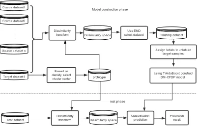
The overall process is shown in Fig.1. The process is divided into four phases. In the first phase, we focus on constructing dissimilarity space. we use the density-based clustering method to calculate the cluster center of samples in the target set, and the prototype set is formed by those cluster center samples. Then, the arc-cosine kernel is used to calculate the sample dissimilarities between the prototype set and the source domain or the target set to form the dissimilarity space. In the second phase, the earth mover’s distance (EMD) method is used to calculate the cost, which is required to convert the data of the source domain, and in the dissimilarity space we select the corresponding samples with a small cost as the training set. In the third phase, we use KNN method to assign labels to unlabeled target samples before building the prediction model, and then The TrAdaBoost method is used to construct the prediction model. Finally, the test set is also mapped into the dissimilarity space to obtain the predicted results.
Figure 1. The framework of the DM-CPDP method
3.1. Dissimilarity Space Construction
To construct a CPDP model in dissimilarity space, we represent the sample by the pairwise dissimilarity between the sample and the prototype set R obtained from the target set
X
T .T
R
p
p
p
R
=
{
1,
2,...,
r}
,
. In dissimilarity space, the set is represented as:r n j i
r
k
x
p
p
p
p
R
X
D
(
,
=
(
1,
2,...,
))
=
[
(
,
)]
(1)Each instance is represented as a r-dimensional dissimilarity vector, k(xi,pj) represents the
dissimilarity between the i-th sample in data set X and the j-th prototype sample in prototype set R. This paper uses the density-based clustering method to select the cluster center as the prototype set, and use the arc-cosine function to measure the pair-wise dissimilarity between sample.
3.1.1. Prototype selection
representative samples in the data set. So we use the DPC method to cluster samples in this stage. The cluster center has two characteristics: high density and large distance. Cluster centers are surrounded by neighbors with lower local density and relatively large distances from other high density points.
In the first step, we calculate the local density
iand local distance
ifor each point.The
iis equal to the number of points that are closer thand
cto point i. The local densitycalculation method is as follows:
−= j
c ij
i
(d d )
(2)The distance
d
ijbetween sample points is measured by Euclidean distance,d
cis the cutoffdistance which ensures each point has at least 2% of the total points as its neighbors, and
d
c
0
. Where
(x)=1 ifx
0
and
(x)=0 otherwise.The local distance calculation method is as follows:
=
=
d
otherwise
imum
the
has
x
if
d
ij j i
i i
ij j i
i j
(
),
max
max
),
(
max
:
(3)
The local distance has two cases: when the point
x
iwith highest local density,
iis the greatestpossible distance with others; Otherwise,
i is the distance fromx
ito the nearest data point withgreater local density.
Then, the cluster center is selected by considering
iandiin combination, the method isshown in formula (3).
iandimay be in different orders of magnitude, we normalize these twoquantities,
z
(
)
is the normalized process. We sort the points in descending order of
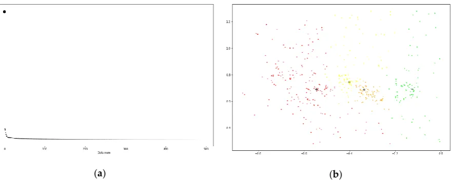
iand represent it in the form of a graph, the graph are shown as Figure2. The value of the non-cluster centers are relatively smooth and there is a clear jump from the non-cluster center to the cluster center, we choose the point above the inflection point as the cluster centers.)
(
)
(
i ii
z
z
=
(4)Algorithm 1 Prototype Selection
Input: mk
T
X
: data from the target setOutput: the prototype
R
rk1 Initialize the current prototypeR
/*computer
d
ij andd
c phase*/2 M =m(m−1) 2 /*M is the number ofdij, due todij =dji,(i j)*/
3 for i = 1, 2, ... , m do
4 for j = i+1, i+2, ... , m do
5 Computer the distance
d
ij by the Euclidean distance7 end
8 sort
M ij
d
in ascending order9 dc(M*0.02)th point distance value
/*cluster center selection phase*/
10 for i = 1, 2, ... , m do /*each sample
x
i belonging toX
Tmk*/ 11 computer the density
iaccording to step 9 and Eq.(2)12 computer the distance
iaccording to Eq.(3)13 computer the candidate cluster center
ias cluster center according to Eq(4)14 end
15 sort
i min descending order16 select all the cluster center as the prototype set R according to step15;
17 return
R
rkThe method is shown in Algorithm1. In step3-7, we calculate the distance between samples, then we sort the distances in ascending order and select the value of the 2%th data as the cut-off distance
d
cin step 6-9. In step 10-14, we calculate the local density
iand local distance
ifor each sample, and calculate the cluster center decision factor
iaccording to
iand
i. Last, we sort
i in descending order to select the cluster centers as the prototype set.(a) (b)
Figure 2. Cluster center selection diagram. (a) is the descending arrangement diagram of i; (b) is the display
of the cluster center point selected by the graph (a) in the data sample
3.1.2. Dissimilarity transformation
of better represent the dissimilarity between vectors, we use k0(x,y)to measure the pair-wise
dissimilarity, short in k(x,y), and shown as:
|| || || || cos 1 1 ) , ( 1 y x y x y x k − = −
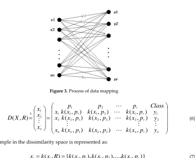
(5)In the transformation process, we first use the arc-cosine kernel function to measure the dissimilarity between each original sample and the prototype set, and these values are used as row vectors, and then the low-dimensional dissimilarity space is constructed. The process is shown in Fig.4 and formula (6). The dimension of this space is determined by the number of samples in the prototype set R. k(xi,pj)represents the dissimilarity between the sample
x
i and the prototypesamplepj.
Figure 3. Process of data mapping
=
=
n r n r r r n n nn
k
x
p
y
y
p
x
k
y
p
x
k
Class
p
p
x
k
p
x
k
x
p
x
k
p
x
k
x
p
x
k
p
x
k
x
p
p
x
x
x
R
X
D
)
,
(
)
,
(
)
,
(
)
,
(
)
,
(
)
,
(
)
,
(
)
,
(
)
,
(
)
,
(
2 21 1 2 1 2 2 1 2 2 2 1 1 1 1 2 1 ' ' 2 ' 1
(6)Each sample in the dissimilarity space is represented as:
)}
,
(
),...,
,
(
),
,
(
{
)
,
(
1 2' r i i i i
i
k
x
R
k
x
p
k
x
p
k
x
p
x
=
=
(7)We use the above method to map each source domain data set and target set into the dissimilarity space, the dissimilarity space construction method is shown in Algorithm2. Step 3-9 is the process of mapping a source domain data set into the subspace. In this stage, '
i
x
is the dissimilarity representation of samplex
i, and is obtained by calculating the dissimilarity betweeneach source data sample and the prototype set. Then we add ' i
x
to the subspaceD(XSu,R). Step 13-17is the process of mapping target set into dissimilarity, the process is the same as the source domain data set. Finally, the dissimilarity space D is obtained by combining these subspace.
Algorithm 2 Dissimilarity Space Construction
Input: XSnk
: data from the source domain data set
k m T
k r
R
: the data of prototype, mk TX R
u: the number of source domain data set
Output: D: dissimilarity space
1 initialize the current D
/*map source domain data sets into D*/
2 for each
X
Sun k
S
do
3 initialize the current D(XSu,R)
4 for each nK
Su i
X
x
do
5 for each rk
j R
p do
6 computer k(xi,pj) according to Eq.(5)
7 end
8 get another representation of sample
x
i:x
i'9 ( , ) ( , ) '
i Su
Su R D X R x
X
D
10 end
11 DDD(XSu,R)
12 end
/*map target data set to D*/
13 for each mK T i
X
x
do14 initialize the current D(XT,R)
15 repeat step 5-8
16 ( , ) ( , ) '
i T
T R D X R x
X
D
17 end
18 DDD(XT,R)
19 Return D
3.2. Selection of Multi-Source data sets
To select the appropriate data sets, the Earth Mover’s Distance(EMD) is used to measure the similarity between the sets. The EMD is defined as the minimum amount of work that required to
Algorithm 3 Selection of multi-source data sets
Input: D(XSu,R):representation of source domain data set
X
Suin space Du: the number of source domain data set in space D
1 for each nr Su R
X
D( , ) in D
2 for each
x
i' in D(XSu,R) do3 computer the move cost
d
ijaccording to Eq.(9)4
computer the optimum solution
f
ij according to Eq.(8) and the restrictions of Eq.(11)5 computer the cost function
D
XSuRaccording to Eq.(10)6 end
7 end
8 sort
D
XSuR
u in descending order9 select the first ɑ data set as the training data set
10 return training data set
convert a data distribution to another, i.e. assuming X is a warehouse containing n mound and R is a warehouse with p empty pits, the similarity between data sets is the minimal cost to move n mound in X to p pits in R.
In the data set X ={(x1,wx1),...,(xi,wxi),...,(xn,wxn)} , each sample
x
i represents a mound, ix
w
represents the quality (weight) ofx
i . Similarly, in the prototype set)}
,
(
),...,
,
(
),...,
,
{(
p
1w
p1p
jw
pjp
rw
prR
=
, each samplep
j represents a pit.w
pj represents the volume(weight) of
p
j.We consider that the quality of each sample in the same set is equal and the total mass is equal
to the total capacity, and the conditions are shown in (8).
d
ijis the cost of movingx
itop
j, thecalculate method is shown in (9),
k
(
x
i,
p
j)
comes from the matrix (7). We consider the cost functionXR
D from X to R as the similarity between the source data set and the prototype set, that is, the similarity between the source data set and the target set. The cost function DXR refer to formula
(10).
=
=
=
=
= = n i r j p x p x j i j iw
w
r
w
n
w
1 11
1
1
(8))
,
(
1
i jij
k
x
p
d
=
−
(9)
= ==
n i r j ij ijXR
d
f
D
1 1
min
(10)ij
f
defines the flow fromx
i top
j, the method hopes to find an optimal solution
f
ij to
=
=
=
= = = = = = n i r j p n i x r j ij n i p ij r j x ij ij j i j iw
w
f
r
j
w
f
n
i
w
f
r
j
n
i
f
1 1 1 1
1 1
}
,
min{
1
,
1
,
1
;
1
,
0
(11)The method of data set selection is shown in Algorithm3. In step 2-6, We calculate the cost function of convert the source domain data set into the same data distribution as the prototype set. In step 8-10, we sort the cost function
D
(
X
Su,
R
)
in descending order, the first ɑ data sets are selected as the training set.3.3. Model Construction
Due to the values of all sample attributes are in [0, 1] after dissimilarity transformation, we can use the KNN method without being affected by noise in the dissimilarity space. Each attribute of the sample represents the degree of dissimilarity between the original sample and the prototype sample in the dissimilarity space, and the more similar to the prototype, the greater value we get. So that the KNN method is suitable for assigning labels in the space. We find k points closest to the target sample and assign a label to the target sample by voting method which is calculated by formula (12). Therefore, statistical-based machine learning algorithms can be used to build prediction models. In order to achieve better transferring, we use the classic TrAdaBoost algorithm to build the prediction model.
)
)
1
(
)
1
(
(
1 1
==
+
−
==
−
=
k i k i ii
I
y
y
I
sign
y
(12))
(
I
is the number of samples marked as positive (negative) in k samples.sign(x)is a symbolic function, where sign(x)=1ifx
0
and sign(x)=0otherwise.4.Experiments
4.1. Data Set
In order to verify the effectiveness of the DM-CPDP method, we validate the performance of the prediction model through experiments and compare it with other methods. In this paper, we selected 14 data sets in NASA and 3 data sets in SOFTLAB to experiment. The data sets of NASA and SOFTLAB are obtained from PROMISE database, and these data sets are shown in Table 1.
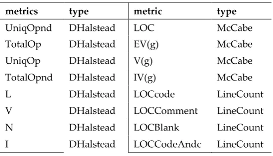
These data sets are derived from different projects, and the data distribution as well as feature attributes are different. We choose the common attributes of the target set and the source domain data set to build the prediction models. Table 2 shows the metrics of the software features used in the experiment. It mainly includes McCabe metric element, Line Countmetric element, Halstead basic metric element, and its extension DHalstead metric element.
To facilitate comparison, we performed two parts of the experiment on the data sets: NASA to NASA, NASA to SOFTLAB.
NASA to NASA: Use the data set in NASA as the target set and use the remaining data sets belonging to NASA as the source domain data sets.
4.2. Performance Index
In this paper, the prediction results are measured according to the indexes of F-measure and AUC. The performance index is calculated based on the confusion matrix shown in Table 3.
Table 1. Data set
Project Examples Defect class %Defective Features
NASA
CM1 327 42 12.84 37
PC1 70 5 61 8.65 37
PC2 745 16 2.15 36
PC3 1563 160 10.24 37
PC4 1287 177 13.75 37
PC5 1723 471 27.34 39
KC1 1183 314 26.54 21
KC2 522 107 20.49 21
KC3 194 36 18.56 39
KC4 125 61 48.80 42
MC1 327 42 12.84 37
MC2 125 55 35.20 39
MW1 253 27 10.67 37
JM1 10878 2105 19.35 21
SOFTLAB
ar3 63 8 12.70 29
ar4 107 20 18.69 29
ar5 36 8 22.22 29
Table2. Software metric element
metrics type metric type
UniqOpnd DHalstead LOC McCabe
TotalOp DHalstead EV(g) McCabe
UniqOp DHalstead V(g) McCabe
TotalOpnd DHalstead IV(g) McCabe
L DHalstead LOCcode LineCount
V DHalstead LOCComment LineCount
N DHalstead LOCBlank LineCount
I DHalstead LOCCodeAndc
omment
D DHalstead B DHalstead
T DHalstead E DHalstead
Table3. Confusion Matrix
Predicted positive Predicted negative
Real positive TP FN
Real negative FP TN
F-measure is determined by both recall and precision, and its value is close to the smaller value of both. So that the larger F-measure means that both recall and precision are larger, the formula is shown in (13), where ɑ is used to regulate the relative importance of precision and recall, and its value is usually at 1.
precision recall
precision recall
) 1 ( measure
-F
+
+ =
(13)
FN TP
TP recall
+
= (14)
FP TP
TP precision
+
= (15)
Recall is the ratio of correctly predicting the number of defective modules to the number of real defective modules, indicating how many positive samples are correctly predicted.
Precision is the ratio between correctly predicting the number of defective modules and the number of all predicted defective modules, indicating how many predictions are correct in positive samples.
AUC is defined as the area under the receiver operating characteristics (ROC) curve, this performance indicator is one of the criteria for judging the two-category model.
4.3. Analysis of results
By comparing with traditional single-source and multi-source defect prediction methods, we prove that establishing prediction models in the dissimilarity space can improve the performance of prediction model, and prove the superiority of the DM-CPDP method. The construction of classifier in the dissimilarity space is mainly influenced by two factors: dissimilarity metric and prototype selection. We compared the effects of different dissimilarity metric and prototype selection methods on the experimental results. In addition, we also verified the necessity of multi-source data in CPDP methods.
4.3.1. Experiment on different methods
In order to verify the superiority of the DM-CPDP method, we compare it with traditional CPDP models.
target set are selected randomly as the training set, and the data of remaining target set are used as the test set. Each experiment was repeated 10 times, and the results were averaged. The experimental details of each method are as follows:
TNB: randomly select a data set as the training set, and assign weights to the training samples according to the target set using data gravity. Finally, the defect prediction model is built using the NB algorithm.
MSTrA: selects multiple data sets as training set and distributes weights for each training data according to the target set using data gravitation. In each iteration, each source domain data set is matched with the target set to train weak classifiers, and the weak classifier in the current iteration with the lowest error rate on the target set is selected.
HYDRA: merge each candidate source and target data set as training set to construct multiple base-classifiers, and then used genetic algorithm to find the optimal combination of base-classifiers. After that, we use a process similar to the AdaBoost algorithm to obtain a linear combination of GA models.
The results are shown in Table 4 and 5.
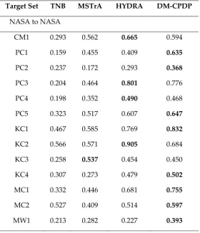
It can be seen that the DM-CPDP method outperforms several existing algorithms on most data sets. In the NASA to SOFTLAB experiments, the performance of each algorithm on SOFTLAB data sets is stable. DM-CPDP method is better than the other algorithms. The average value of F-measure and AUC are 2.8%-27.3% and 1.7%-7.8% higher than other algorithms, respectively.
In the NASA to NASA experiment, the average value of our method on F-measure and AUC are higher than other methods 4.4%-28.8%, 5.5%-13.0%. On the two index of F-measure and AUC, the DM-CPDP method performs optimally on 9 data sets, HYDRA performs optimally on 4 data
Table 4. Comparison of performance indicators F-measure
Target Set TNB MSTrA HYDRA DM-CPDP
NASA to NASA
CM1 0.293 0.562 0.665 0.594
PC1 0.159 0.455 0.409 0.635
PC2 0.237 0.172 0.293 0.368
PC3 0.204 0.464 0.801 0.776
PC4 0.198 0.352 0.490 0.468
PC5 0.323 0.517 0.607 0.647
KC1 0.467 0.585 0.769 0.832
KC2 0.566 0.571 0.905 0.684
KC3 0.258 0.537 0.454 0.450
KC4 0.307 0.273 0.479 0.502
MC1 0.332 0.446 0.681 0.755
MC2 0.527 0.409 0.514 0.597
JM1 0.396 0.563 0.595 0.811
average 0.320 0.442 0.564 0.608
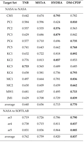
NASA to SOFTLAB
ar3 0.416 0.708 0.755 0.781
ar4 0.509 0.714 0.713 0.753
ar5 0.652 0.809 0.846 0.863
average 0.526 0.743 0.771 0.799
Table 5. Comparison of performance indicators AUC
Target Set TNB MSTrA HYDRA DM-CPDP
NASA to NASA
CM1 0.642 0.674 0.793 0.782
PC1 0.584 0.596 0.624 0.810
PC2 0.557 0.535 0.576 0.563
PC3 0.629 0.686 0.879 0.842
PC4 0.577 0.710 0.696 0.735
PC5 0.741 0.643 0.662 0.768
KC1 0.632 0.722 0.818 0.892
KC2 0.776 0.813 0.857 0.853
KC3 0.733 0.565 0.689 0.685
KC4 0.658 0.581 0.756 0.793
MC1 0.497 0.664 0.781 0.836
MC2 0.630 0.609 0.659 0.662
MW1 0.681 0.657 0.495 0.715
JM1 0.629 0.708 0.729 0.839
average 0.640 0.656 0.715 0.770
NASA to SOFTLAB
ar3 0.719 0.726 0.786 0.790
ar4 0.738 0.715 0.811 0.837
ar5 0.831 0.836 0.864 0.885
sets. The MSTrA method performs best on F-measure only one data set, and the TNB method performs best on AUC only one data set. The reason of which is that the influence of data distribution. Different machine learning methods behave differently on the same data set, and the same machine learning method performs differently on different data sets. But it is still superior to other algorithms in general. By comparing with these three classic CPDP methods, it can be proved that DM-CPDP method performs well in the field of CPDP.
4.3.2. Experiments on Multi-source data sets and dissimilarity space
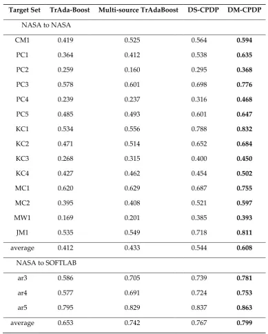
Table 6. F-measure value of different model construction methods
Target Set TrAda-Boost Multi-source TrAdaBoost DS-CPDP DM-CPDP
NASA to NASA
CM1 0.419 0.525 0.564 0.594
PC1 0.364 0.412 0.538 0.635
PC2 0.259 0.160 0.295 0.368
PC3 0.578 0.601 0.698 0.776
PC4 0.239 0.237 0.316 0.468
PC5 0.485 0.493 0.601 0.647
KC1 0.534 0.556 0.788 0.832
KC2 0.471 0.514 0.652 0.684
KC3 0.268 0.315 0.400 0.450
KC4 0.427 0.462 0.454 0.502
MC1 0.620 0.629 0.687 0.755
MC2 0.395 0.408 0.521 0.597
MW1 0.169 0.201 0.385 0.393
JM1 0.535 0.549 0.718 0.811
average 0.412 0.433 0.544 0.608
NASA to SOFTLAB
ar3 0.586 0.705 0.739 0.781
ar4 0.577 0.691 0.724 0.753
ar5 0.795 0.829 0.837 0.863
average 0.653 0.742 0.767 0.799
Table 7. AUC value of different model construction methods
Target Set TrAda-Boost Multi-source TrAdaBoost DS-CPDP DM-CPDP
CM1 0.639 0.662 0.716 0.782
PC1 0.592 0.601 0.723 0.810
PC2 0.519 0.532 0.531 0.563
PC3 0.640 0.669 0.715 0.842
PC4 0.568 0.689 0.683 0.735
PC5 0.625 0.631 0.725 0.768
KC1 0.711 0.724 0.841 0.892
KC2 0.797 0.806 0.819 0.853
KC3 0.518 0.574 0.596 0.685
KC4 0.570 0.577 0.628 0.793
MC1 0.633 0.654 0.746 0.836
MC2 0.549 0.593 0.615 0.662
MW1 0.627 0.651 0.684 0.715
JM1 0.665 0.701 0.782 0.839
average 0.618 0.641 0.700 0.770
NASA to SOFTLAB
ar3 0.684 0.734 0.752 0.790
ar4 0.629 0.714 0.741 0.837
ar5 0.717 0.810 0.856 0.885
average 0.677 0.753 0.783 0.837
In order to verify the impact of multi-source data and sample dissimilarity representation on the performance of predictive models, we compare the TrAdaBoost, Multi-source TrAdaBoost, Dissimilarity space based Single-source CPDP (DS-CPDP) method, and DM-CPDP method on F-measure and AUC respectively. Each experiment was repeated 10 times, and the results were averaged. The experimental details of each method are as follows:
TrAdaBoost: randomly select 90% of the source domain data set and target set as the training set, and the remaining target set as the test set. The prediction model was then built using TrAdaBoost.
Multi-source TrAdaBoost: before using the TrAdaBoost algorithm to build a prediction model, the EMD method is used to select multiple data sets that are highly correlated with the target set, then these data sets are combined with the target set as a training set. Finally, the TrAdaBoost algorithm is used for modeling.
DS-CPDP: randomly select a data set from the source domain for dissimilarity transformation as the training set, and then use KNN method to assign labels to unlabeled target, after that use the TrAdaBoost method to build model.
The experimental results are shown in Table 6, 7.
dissimilarity space. The average value of F-measure is higher than the DS-CPDP method by 6.4% and 3.2% in the two series of data sets respectively. The average value of AUC is higher than the DS-CPDP method by 7.0% and 5.4%. By comparing the results of TrAdaBoost and Multi-source TrAdaBoost, we can find that the Multi-source TrAdaBoost method is better than the TrAdaBoost in the feature space, and the average value of F-measure is higher than the TrAdaBoost method by 2.1% , 8.9%, the average value of AUC is higher than the TrAdaBoost method by 2.3%, 7.6%. These results prove that the CPDP method based on multi-source data can improve the performance of prediction models, whether in the dissimilarity space or in the feature space.
In order to verify that the construction of dissimilarity space can improve the performance of the classifier, we compare these two sets of experiments: TrAdaBoost and DS-CPDP, Multi-source TrAdaBoost and DM-CPDP. From the experimental results in Table 6 and 7, the average value of DS-CPDP on F-measure is 13.2% and 11.4% higher than that of TrAdaBoost algorithm respectively. And the average value on AUC is higher than the latter by 8.2%, 10.6%. By comparing DM-CPDP with Multi-source TrAdaBoost, we can find that the former is better than the latter in the average value of the two performance indicators. And the average value of F-measure in the former is higher than that in the latter 17.5% and 5.7% respectively. In terms of AUC, the former is better than the latter 12.9% and 8.4% respectively. Therefore, it can be proved that the model established in the dissimilarity space is better than that built in the feature space.
The reasons for these results are as follows: (1) Multi-source data sets highly related to the target set are more likely to satisfy the hypothesis of data distribution in the data transferring and reduce the effect of source component shift. (2) the amount of useful information in the training set will affect the performance of the model to a certain extent. (3) when using source domain and target domain data to construct dissimilarity space, each sample is represented as the dissimilarity between the sample and the prototype set, and the smaller dissimilarity is, the larger attribute value we get, so that these samples with high similarity to the target set will gain higher attention during the modeling process, and thus improve the performance of the classifier.
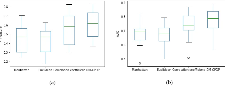
4.3.3. Different Dissimilarity Metric Method
In this part , we compare the effects of several different dissimilarity metric methods on the experimental results, verifying which of the most efficient measurement in CPDP.
Figure 4. is the box plot of performance indicators, which compare the values of several different dissimilarity metric methods on F-measure and AUC. We choose Euclidean distance, Manhattan distance , and correlation coefficient as the measurement of dissimilarity.
(a) (b)
The experimental results show that the prediction model using Manhattan distance and Euclidean distance as the measurements of dissimilarity are poor. The value of median, quartile, maximum, and minimum on F-measure and AUC are lower than the arc-cosine kernel. And during the course of the experiment, we found that the average values of the arc-cosine kernel methods on F-measure and AUC are still higher than those two methods. In addition, it can be seen from the box plot that when we use the correlation coefficient as a measure method, the value of median, quartile, maximum, and minimum on F-measure and AUC are still lower than the arc-cosine kernel, but higher than the Manhattan and Euclidean distances. And the average value of F-measure and AUC are lower than the kernel method we use.
The reason for these results is that when the relationship between samples is measured by Euclidean distance and Manhattan distance, if the sample and the prototype are highly correlated, the attribute value of the sample in the dissimilar space is lower, so that the samples with the same distribution to the target set data receive less attention in the process of modeling. Correlation coefficient as the measurement is opposite to the above two methods, this method makes the same distribution samples get higher attention when building the classifier. But these three methods are inferior to the arc-cosine kernel method. So it can be concluded that using the arc-cosine kernel function as the measure method of dissimilarity between samples works better, and the effect of this method is more stable.
4.3.4. Different prototype set selection methods
In this part, we compare the effects of several different prototype set selection methods on the experimental results.
Figure 5. compare three different methods of prototype set selection, namely random algorithm, the K-means algorithm, and the DPC method for DM-CPDP. For random methods, generally select 3%-10% of the data set [26]. When using the random method to select the prototype set, we select r samples as the prototype set,r=logI (I is the number of the instance), and repeat the results 10 times to take the mean. When using the K-means method, we also select r samples as the initial cluster center for clustering, and select the output cluster center as the prototype set.
It can be seen from box plot that the density-based prototype selection method used in this paper is better than the random selection method and the K-means clustering method. In Fig.7 and Fig.8, the density-based prototype selection method used by the DM-CPDP has higher value of median, quartile, maximum, and minimum on the F-measure and AUC than the other two methods. However, the K-means clustering method performs the worst, and this method is not suitable for prototype selection.
(a) (b)
Figure 5. Box plot of different prototype selection method. (a) is the situation of each method on F-measure; (b) is the situation of each method on AUC. Box plots represent maximum, upper quartile, median, lower quartile and minimum values from top to bottom. In addition, circles represent outliers.
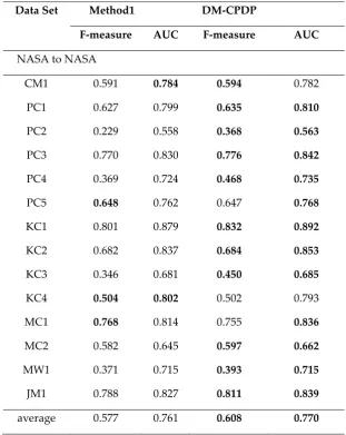
4.3.5. Experiment on different data set selection methods
In this part of the experiment, we compare the effects of different data set selection methods on the experimental results.
Table 8. Different data set selection method
Data Set Method1 DM-CPDP
F-measure AUC F-measure AUC
NASA to NASA
CM1 0.591 0.784 0.594 0.782
PC1 0.627 0.799 0.635 0.810
PC2 0.229 0.558 0.368 0.563
PC3 0.770 0.830 0.776 0.842
PC4 0.369 0.724 0.468 0.735
PC5 0.648 0.762 0.647 0.768
KC1 0.801 0.879 0.832 0.892
KC2 0.682 0.837 0.684 0.853
KC3 0.346 0.681 0.450 0.685
KC4 0.504 0.802 0.502 0.793
MC1 0.768 0.814 0.755 0.836
MC2 0.582 0.645 0.597 0.662
MW1 0.371 0.715 0.393 0.715
JM1 0.788 0.827 0.811 0.839
NASA to SOFTLAB
ar3 0.765 0.779 0.781 0.790
ar4 0.724 0.782 0.753 0.837
ar5 0.848 0.869 0.863 0.885
average 0.779 0.810 0.799 0.837
Since the samples have been mapped into the dissimilarity space, the data set selection method based on extracting the feature vectors is no longer applicable. But we also compare the EMD with another method. In each dissimilarity subspace, we select the value of the smallest attribute in each sample and take the mean value to measure the similarity between the source domain data set and the prototype set. Sort the values in descending order and select the first ɑ data sets as the training data. We call this approach as Method 1. The calculation is as follows:
r j n i p
x k n
D
n
i
j i r
XR =
= min ( , ) 1 ,1
1
1
(16)
The experimental results are shown in Table 8. The results show that the performance of data set selection method based on EMD is superior to Method1 in F-measure and AUC. The reason for this phenomenon is that when comparing the similarity between data sets, Method 1 has lost more information by selecting the minimum attribute and averaging these attribute values. Which leads to inaccurate measurement results. However, the EMD method takes into account each attribute of the sample, so the performance of the prediction model is better.
5. Threats to Validity
The main factor affecting the internal validity of the experiment is the deviation in the code implementation process. For example, we use the HYDRA algorithm for comparison, the algorithm needs to use the genetic algorithm in the implementation. But the random factors of the genetic algorithm may deviate from the experimental results. In view of this problem, this paper eliminates the randomness of the algorithm through repeated tests in the code implementation process. In addition, we compare the results of the reproduce algorithm with the data in the previous papers, which is basically consistent with the results in the previous papers.
The factors that influence the external validity of the experiment are the quality of the data sets and generalization. In view of the quality problem of data set, we choose NASA and SOFTLAB from PROMISE, which are publicly available data sets often used by researchers. Each data set contains different project data to reduce the overall impact of data quality on experimental results. In terms of generalization, the data we used to train the model were derived from two open source data sets. These two open source data sets contain 17 project data for a total of 19458 samples, which guarantee the credibility of the experimental.
6. Conclusion
The contribution of this paper is to put forward the method of establishing the cross-project defect prediction module in the dissimilarity space, which provides a new research idea for CPDP. The basic idea of this paper is to use the density-based clustering method to automatically select the cluster centers from the target set as the prototype set. Then the arc-cosine kernel is used to calculate the dissimilarity between the prototype set and the source domain sample as well as the target sample to form the dissimilarity space. After that the training data set are selected by the EMD method, which calculates the cost of convert the data distribution in the source domain to the same data distribution as the target set, and the corresponding samples with a small cost are selected as the training set in the dissimilarity space. Finally, the prediction model is established by TrAdaBoost algorithm.
In the whole data processing process, we complete two transferring. The first transferring is the dissimilarity measure between samples. In the dissimilarity space, each attribute of each sample is the pairwise dissimilarity between the source domain sample and the prototype sample, and the source domain samples with high correlation to the prototype set have higher measurement values. This method is more flexible than the traditional method of assigning weights to the samples in the feature space. The second transferring is the selection stage of the data sets. In this stage, we make full use of the representation method of samples in the dissimilarity space and use the EMD method to measure the similarity between source domain data set and the prototype set. Experiments show that the DM-CPDP method has better prediction performance than the traditional methods.
Author Contributions: S.R. conceived the idea; W.Z., S.R. performed the experiments and analyzed the results; S.R., W.Z. wrote the initial manuscript; S.R., W.Z., H.S.M., L.X. revised the manuscript together.
Funding: This research was funded by the Central South University Graduate Research Innovation Project under Grant 2018zzts608.
Conflicts of Interest: The authors declare no conflicts of interest.
References
1. Zimmermann, T.; Nagappan, N.; Gall, H. et al. Cross-project defect prediction: a large scale experiment on data vs. domain vs. process. In Symposium on the Foundations of Software Engineering, Amsterdam, The Netherlands, 24-28 August 2009, 91-100.
2. Chen, X.; Gu, Q.; Liu, W.S. et al. Research on static software defect prediction method. Journal of Software. 2016, 27, 1-25, 10.13328/j.cnki.jos.004923.(in chinese)
3. Catal, C.; Software fault prediction: A literature review and current trends. Expert Systems with Applications. 2011, 38, 4626-4636, 10.1016/j.eswa.2010.10.024.
4. Porto, f.; Minku, L.; Mendes, E. et al. A systematic study of cross-project defect prediction with meta-learning. IEEE TSE. 2018, 1-23, arxiv.org/abs/1802.06025.
5. Li, Y.; Huang, Z. Q.; Wang, Y. et al. Cross-project software defect prediction based on multi-source data. Journal of Jilin University. 2016, 46, 2034-2041, 10.13229/j.cnki.jdxbgxb201606037. (in chinese)
6. Pekalska, E.; Duin, R.P.W. Dissimilarity-based classification for vectorial representations. International Conference on pattern recognition, Hang Kong, China, 20-24 August, 2006, 137-140.
7. Cheplygina, V.; Tax, D.; Loog, M. Dissimilarity-Based ensembles for multiple instance learning, IEEE Transactions on Neural Networks and Learning Systems. 2016, 27, 1379-1391, 10.1109/TNNLS.2015.2424254.
8. Ma, Y.; Luo, G.; Zeng, X. Transfer learning for cross-company software defect prediction. Information and Software Technology. 2012, 54, 248-256, 10.1016/j.infsof.2011.09.007.
10. Yu, X.; Liu, J.; Fu,M. et al. A multi-source TrAdaBoost approach for cross-company defect prediction, International Conference on Software Engineering & Knowledge Engineering, San Francisco Bay, USA, 1-3 July 2016, 237-242.
11. Tax, D.M.J. ; Loog, M.; Duin, R.P.W. et al. Bag dissimilarities for multiple instance learning, International Workshop on Similarity-based Pattern Recognition, Venice, Italy, 28-30 September 2011, 222-234.
12. Ren, S.; Zhang, Z.; Liu, Y. et al. Genetic Algorithm-based Transfer Learning for Cross-Company Software Defect Prediction. Journal of Systems & Software. 2017, 10, 45-56, doi.org/10.14257/ijhit.2017.10.3.05 .
13. Yao, Y.; Doretto,G. Boosting for transfer learning with multiple sources. Computer Vision & Pattern Recognition. 2010, 238, 1855-1862, 10.1109/CVPR.2010.5539857.
14. Pekalska, E.; Duin, R. P. W.; Wang, G. Dissimilarity representations allow for building good classifiers. Pattern Recognition Letter. 2002, 23, 943-956, 10.1016/S0167-8655(02)00024-7.
15. Zhang, X.; Song, Q.; Wang, G. A dissimilarity-based imbalanced data classification algorithm. Applied Intelligence. 2015, 42, 544-565, 10.1007/s10489-014-0610-5.
16. Kamei, y.; Fukushima, T.; Mcintosh, S. et al. Studying just-in-time defect prediction using cross-project models. Empirical Software Engineering. 2016, 21, 2072- 2106, 10.1007/s10664-015-9400-x.
17. Fukushima, T.; Kamei, y.; Mcintosh, S. et al. An empirical study of just-in-time defect prediction using cross-project models, Working Conference on Mining Software Repositories, Hyderabad, India, May 31 - June 01, 2014, 172-181.
18. Xia, X.; Lo, D.; Pan, S.J.; Nagappan, N. HYDRA: Massively compositional model for cross-project defect prediction. IEEE Transactions on Software Engineering. 2016, 42, 977-998, 10.1109/TSE.2016.2543218.
19. Yao, Y.; Doretto, G. Boosting for transfer learning with multiple sources. 2010 IEEE Computer Society Conference on Computer Vision and Pattern Recognition, San Francisco, CA, USA, 13-18 June 2010 , 1855-1862.
20. He, J.; Meng, S.; Chen, X. et al. A semi-supervised integration cross-project software defect prediction method. Journal of Software. 2017, 28, 1455-1473, 10.13328/j.cnki.jos.005228.(in Chinese)
21. Plasencia, Y.; Li, Y.; Duin, R. A compact Representation of multiscale dissimilarity data by prototype selection. Iberoamerican Congress on Pattern Recognition. 2016, 150-157, 10.1007/978-3-319-52277-7_19.
22. Shang, Z.; Zhang, L. Software Defect Prediction Using Dissimilarity Measures. Pattern Recognition, Chongqing, China,September 2010, 1-5. (in Chinese)
23. Rodriguez, A.; Laio, A. Clustering by fast search and find of density peaks. Science. 2014, 344, 1492-1496, doi.org/10.1126/science.1242072 .
24. Cho, Y. Kernel methods for deep learning. Advances in Neural Information Processing Systems. 2009, 28, 342-350, 10.1021/ed028p10.
25. Liu, W.; Chen, X.; Gu, Q. Feature selection method based on cluster analysis in software defect prediction. Chinese Science: Information Science. 2016, 46, 1298-1320, 10.1360/N112015-00276.(in Chinese)