Practical Interference Alignment in the Frequency
Domain for OFDM-based Wireless Access Networks
Adrian Loch
∗, Thomas Nitsche
†§, Alexander Kuehne
‡, Matthias Hollick
∗, Joerg Widmer
†and Anja Klein
‡ ∗Secure Mobile Networking Lab, TU Darmstadt, Germany, E-Mail:{adrian.loch, matthias.hollick}@seemoo.tu-darmstadt.de‡Communications Engineering Lab, TU Darmstadt, Germany, E-Mail: {a.kuehne, a.klein}@nt.tu-darmstadt.de †Institute IMDEA Networks, Madrid, Spain, E-Mail:{thomas.nitsche, joerg.widmer}@imdea.org
§Universidad Carlos III, Madrid, Spain
Abstract—Interference alignment (IA) is often considered in the spatial domain in combination with MIMO systems. In contrast, aligning interference in the frequency domain among multiple subcarriers can also benefit single-antenna OFDM-based access networks. It allows for flexible operation on a per-subcarrier basis. We investigate the gains achievable by frequency IA in practice for a scenario with multiple access points and clients. Previous work is predominantly theoretical and focuses on idealized cases where all nodes have the same average signal-to-noise ratio (SNR). On the contrary, in practical networks, nodes typically have heterogeneous SNRs depending on channel condi-tions, which might have a significant impact on IA performance. We tackle this problem by designing mechanisms that adaptively choose which nodes shall perform IA on which subcarriers depending on current channel conditions. We implement and validate our approach on software-defined radios. To the best of our knowledge, this is the first practical implementation of IA in the frequency domain. Our measurements show that (1) frequency IA is feasible in practice, and (2) choosing appropriate nodes and subcarriers overcomes the main limitations due to heterogeneous SNRs. Our mechanisms enable IA in scenarios where it would be infeasible otherwise, achieving throughput gains close to the 33% theoretical maximum.
I. INTRODUCTION
While the latest advances in signal processing and informa-tion theory contribute promising techniques to keep up with the increasing throughput demands in wireless access networks, the implied assumptions often pose a significant challenge for practical deployments. Such assumptions typically include knowledge of full Channel State Information (CSI), frequency and time synchronization of nodes, and operation in the high signal-to-noise ratio (SNR) regime. Adapting state-of-the-art theoretical approaches to practical scenarios is a major hurdle itself which requires complex solutions. Work in this direction has enabled practical implementations of, e.g., MIMO [1], joint multi-user beamforming [2], and random network coding [3].
In information theory, a very recent and promising ap-proach is Interference Alignment (IA) [4], which allows to achieve an increased Degree-of-Freedom (DOF). This means that, in a system withK interfering transmitter-receiver pairs, each pair gets more than a 1/K resource share. Thus, the sum of all shares is larger than one. This surprising result was first established by Cadambe and Jafar in [4]. The key idea behind IA is to align interfering signals into the same subspace, while desired signals lie in orthogonal subspaces. Hence, receivers can decode the desired signal by
combin-ing “aligned” unknowns in an underdetermined system of equations. To achieve alignment, signals are precoded at the transmitters based on CSI. For random channels, IA in the time or frequency domain requires so-calledsymbol extensions, which means that IA is done over multiple time slots or subcarriers. The additional “symbols” provide overflow space for interference that does not align perfectly. The achievable DOF increases with larger extensions but is upper-bounded by 1/2DOF per user. Moreover, the larger the extension, the higher the required SNR [5]. Still, for three transmitter-receiver pairs and the smallest possible extension, which comprises three symbols, a total of four packets can be sent using only three symbols, which translates into a 33% gain compared to no IA. Specifically, alignment allows the first pair to exchange two packets, while the second and third pair exchange one.
The channel coefficients of all symbols in the extension are needed at the senders to ensure alignment. For time extension, this means knowingfutureCSI, which limits its practicability. IA in space is also possible but requires multiple antennas. In contrast, IA in frequency allows to estimate multiple carriers in parallel using only one antenna. Hence, frequency IA is directly applicable to the vast majority of nowadays wireless networks, which are based on Orthogonal Frequency-Division Multiplexing (OFDM) and thus allow for IA over multiple subcarriers. This wide applicability motivates our research on practical IA in the frequency domain. Still, wireless access networks pose a critical problem to IA, since users experience
heterogeneous SNRs, while IA requires (a) similar and (b)
high SNRs [6]. Such heterogeneity may potentially cancel out IA gains completely. In this paper, we investigate schemes to overcome these limitations in a practical 802.11-like network.
In particular, instead of forcing all users tosimultaneously
participate in IA, we propose multiple high-granularity selec-tion algorithms to choose which transmitters shall send data to which receivers on which subcarriers using IA. Moreover, if channel quality makes IA infeasible, we allow to switch per subcarrier to more robust mechanisms such as plain OFDM. In other words, we provide mechanisms to adapt IA to the current channel status. This allows us to achieve lower bit error rates (BERs), which makes IA feasible altogether and translates into a higher throughput. Furthermore, to the best of our knowledge, our system is the first implementation of IA in frequency. Concretely, our contributions are as follows:
• We show that using selection IA performs closely to the theoretical boundaries, with better robustness and stability compared to plain IA without selection algorithms.
• We implement frequency IA along with our selection algorithms on a software-defined radio (SDR) platform.
• We deal with real-world effects such as carrier-frequency offset (CFO), synchronization and channel quantization.
We first present related work and explain how frequency IA works in Section II. Then, in Section III, we give an overview on how our wireless access network based on IA operates. We delve into the details of our selection algorithms in Section IV. In Section V we explain how we deal with practical issues. We present our measurements in Section VI and discuss them in Section VII. Finally, we conclude the paper in Section VIII.
II. RELATEDWORK ANDBACKGROUND
A. Related work
The principle of IA can be applied in the dimensions of time [4], frequency [4], [7], space [8], [9], [10], [11], [12], and signal level [13]. In recent years, the practical imple-mentation of IA schemes has drawn significant attentation, yet remains challenging. [14] provides an overview of practical hurdles for IA, including simulation results based on testbed measurements of MIMO channels. In [15], the spatial IA scheme presented in [8] is validated in a MIMO testbed with up to four antennas per node for the three-user interference channel. In [16], the IA scheme of [8] is combined with interference cancellation, under the assumption that access points are connected via an Ethernet backbone. The proposed scheme is validated in GNU Radio on a testbed of 20 USRP nodes, each equipped with two antennas. An alternative spatial IA scheme named blind IA [11], [12] was implemented in [17] on SDRs on top of an OFDM physical layer. In blind IA, which does not require CSI at the transmitter, there are two transmitting nodes, each with one antenna, and two receiving nodes, each with two antennas among which it is possible to
switch. Alternating both receive antennas enables IA without
CSI feedback. Blind IA has also been implemented on the FPGA-based SDR Wireless Open-Access Research Platform (WARP) developed at Rice University [18] in [19]. In [20], a spatial IA scheme based on [9] is implemented and validated for 2 ×2 MIMO IA with 3 users on USRPs using OFDM at the physical layer. Although some of the aforementioned work uses OFDM, the actual IA does not take place in frequency but in space, thus requiring multiple antennas. However, there exists work on practical issues ofIA in frequency. In [21], it is shown that strict alignment conditions can be weakened in practice if the “perfect” IA requirement is relaxed to “best-effort” IA. In [5], the use of lattice decoding instead of zero-forcing is discussed for various IA schemes such as the frequency IA approach presented in [4]. Sphere decoding allows to reduce the BER of IA significantly when compared to conventional zero-forcing, thus enabling IA for lower SNRs. However, this performance improvement comes at the cost of a highly complex receiver whose practicability has not yet been studied. In [22], the performance of frequency IA is evaluated offline using jointly measured radio channels from three base stations in an urban macrocell scenario. Still, note that none of these works implements functional frequency IA on a testbed, nor proposes selection schemes to enable it in practice.
B. Background on IA in the frequency domain
We briefly summarize frequency IA. We consider the K= 3case and a symbol extension overNP = 3subcarriers, since our schemes build on this setting. The general case for NP = 2c+ 1 subcarriers with c ∈ N can be found in [4]. In our setting, transmitter 1 encodes two packets, x1 andx2,
represented by a2×1column vectorxSwith precoding matrix V1 ∈ C3×2, i.e., V1 is composed of two precoding vectors
having the size of the symbol extension, one for each packet in xS. Transmitters 2 and 3 encode only one packet each,
denoted asx3andx4with precoding matricesV2,V3∈C3×1, respectively. In other words, each transmitter sends the same data over all three subcarriers, but precoded with a different value. Transmitter 1 sends a linear combination ofx1andx2,
that is, x1V1,1+x2V1,2,V1,k being thek-th column ofV1.
At the receiver side, each node receives the superposition of all transmitted signals on each of the three subcarriers. As a result, each receiver has three times the same overlapped data but affected by different channel coefficients, i.e., each receiver has a system of three linearly independent equations. Still, there arefourunknowns, one for each packet. Specifically, the received signal rn at the n-th receiver can be written as
rn =Hn1V1xS+Hn2V2x3+Hn3V3x4+zn (1)
with the 3×3 matrix Hnm = diag(hnm[1], hnm[2], hnm[3]) m, n ∈ [1,2,3], where hnm[i] denotes the complex channel coefficient of the channel from transmittermto receivernon subcarrieriandzn ∼ CN(0,1)denotes Additive White Gaus-sian Noise (AWGN) at receivern. To solve the aforementioned linear system, two of the four packets need to be aligned. As a result, they occupy a common signal space and can be combined to one unknown representing interference, yielding a solvable system of three equations and three unknowns. One solution is discarded, as it is the sum of two interfering signals, but the other two packets can be decoded. We use a design for the precoding matrices [4] which allows to decodex1 andx2
at receiver 1,x3at receiver 2 andx4at receiver 3. In particular, V1= [w T1w],V2=T2w andV3=T3T1w, where
T1 = H12(H21)−1H23(H32)−1H31(H13)−1, (2)
T2 = (H32)−1H31, (3)
T3 = (H23)−1H21, (4)
andwis the3×1initial precoding vector, which can be chosen freely. As suggested in [4], we define w as an all-one vector. At receiver n, the interference is zero-forced using the 3×3
zero-forcing filter matrix An = (Bn)−1, which is designed according to the precoding matrices. More precisely, the k-th column Bn,k of matrixBn is given by
Bn,k=
( H
n1V1,k k= 1,2
Hn2V2 k= 3 ∪ n= 1,2 H33V3 k= 3 ∪ n= 3
(5)
with V1,k denoting the k-th column of precoding matrix V1.
Essentially,Bncontains the three aforementioned equations at the receivers, i.e., with aligned interference. To solve the linear system, we invert Bn and multiply the result by the received data. The outcome is the zero-forced signalsn, which contains the original packets x1, x2, x3 and x4 (c.f. Section IV-A2).
III. SYSTEMMODEL
Next, we explain the operation of a wireless access network that uses IA for the downlink. We do not consider the uplink because throughput demands are typically significantly lower and thus the effort required for IA does not pay off. We assume a scenario with maccess points (APs) andn mobile stations (MSs) which are randomly distributed. The APs are connected to a wired backbone which allows them to synchronize. We assume that all APs have data to send to all MSs. This setting can be considered realistic since throughput demands on the downlink are typically high. APs can exchange data packets via the backbone and can thus deliver them to any MS. All APs and MSs are in each other’s range, share the same bandwidth and use OFDM with N subcarriers. As a baseline, we use
plain OFDM, i.e., all nodes use OFDM over allsubcarriers. MSs are served in a time-division manner, that is, one at a time, by the AP to which their average SNR is best.
A. IA operation
We consider IA in the frequency domain as described in Section II, i.e., an IA scheme which allows three transmitters to sendfourstreams to three receivers using onlythreeOFDM subcarriers. To deploy such a scheme in a network, nodes need to be arranged in groups of six, i.e, three APs and three MSs. The throughput performance of the scheme is directly related to the channel quality of the links in each group. Hence, arranging nodes in groups which are beneficial for IA is key to achieve the theoretical 33% gain. Since we implement IA in the frequency domain, nodes can also be grouped per subcarrier. For ease of exposition, we use the following terms to refer to the different types of grouping we perform to optimize IA:
• Node group. We define as node groups the aforemen-tioned3×3node sets including three APs and three MSs.
• Subcarrier combination. We call a subcarrier combina-tion the set of three subcarriers used for IA.
• Node pair. We call a nodepair two nodes exchanging a data stream using IA within a node group.
• Node subset. We definesubsetsas portions of them×n access network which are larger than a3×3node group.
Exploiting the wireless access network scenario and the aforementioned backbone, IA allows to optimize the following:
1) Node Selection. Distinct subcarrier combinations can be allocated to different3×3 groups. Thus, different nodes can simultaneously use different parts of the spectrum. 2) Subcarrier Selection. Nodes can choose which
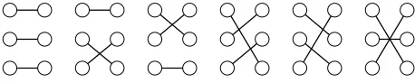
subcar-rier combinations to use. Ideally, IA works best when the channels of a combination are linearly independent. 3) Stream Selection. Within a node group using a certain
subcarrier combination, we can choose which transmitter sends to which receiver. There are six possible pairings (Figure 1). Note that APs can exchange packets. Thus, packets can be delivered regardless of the chosen pairings. 4) Mechanism Selection. APs can decide to resorton
cer-tain subcarriersto plain OFDM or any other alternative
mechanism if IA cannot perform well with the given CSI.
WeestimateIA performance for eachpossible node,
sub-carrier, stream, and mechanism selection to find the best one. To make this exhaustive search tractable, we use heuristics that reduce the complexity of the resulting combinatorial problem.
B. Heuristics for scalable selection
1) Subcarrier Selection: The number of possible
combina-tions of three subcarriers is given by the binomial coefficient N
3
. While 802.11g only has 48 subcarriers, which leads to
17296possible combinations, 802.11n or 802.11ac feature 112 and 484 subcarriers respectively, what causes the number of combinations to exceed 18 million. Estimating IA performance for each combination to find the best one is infeasible. We propose exploiting the nature of wireless channels to overcome this problem. While subcarriers behave similar if they are close to each other in the frequency domain, they are likely uncorrelated when they are far apart enough. This effect is known as the coherence bandwidth BC. To ensure that subcarriers are uncorrelated, we only need to allocate them sufficiently far apart, that is, further than BC. Assuming an indoor propagation delay spread of at most 700 ns [23], BC≈ 7001ns = 1.42MHz. In 802.11g/n/ac, subcarrier spacing is 312.5 KHz. Hence, there must be at least d1.42MHz
312.5KHze = 5 subcarriers in between subcarriers of the same combination.
Forming combinations.We thus define a fixed allocation of combinations which maximizes the spacing between sub-carriers of the same combination. More precisely, subcarrier i is always combined with subcarriers N3 +i and 2·3N +i, for i∈
1. . .N3 −1. For 802.11g this means that subcarriers of a combination are separated 5MHz> BC. For 802.11n/ac, the separation is even larger, as there are more subcarriers. Note that this does not ignore frequency selective fading, since we still do subcarrier-wise node, stream, and mechanism selection. Subcarrier selection would just add a dimension but incurs in the aforementioned unfeasibly large number of combinations.
2) Node Selection: IA needs to select3×3node groups out
of them×nnodes available in the network. A straightforward approach would measure CSI of all m×n links and find the best group of six nodes. Still, drawbacks are (a) the number of possible node groups gets unmanageably large with increasing network size, (b) all links are constantly measured, which causes overhead, and (c) if we always choose the best network-wide group, nodes at adverse locations in terms of CSI might not be served at all. Hence, we propose to split the network into smaller subsets and serve each subset one at a time. This reduces the combinatorial problem, as we only need to search within each subset the3×3group that optimizes performance.
Forming subsets. IA works best if each MS in a node group has (a) homogeneous, and (b) high SNRs to each AP in the group [6]. While finding optimal schemes to divide anm×
nnetwork into subsets of sizems×nsis beyond our scope, we propose a greedy heuristic which provides suitable subsets. We divide themAPs into sets ofmsAPs each. Broadly speaking, the goal (a) is fulfilled by MSs at similar distances to all ms APs, and the goal (b) requires MSs to be close to the APs. Thus, we cluster APs which are close to each other, since then the equidistant point to all APs is also close to them.
Next, we calculate at each MS the average SNR to each AP in each set of APs. That is, at each node we obtain bm/msc sets ofmsSNR values. Then, each node associates in a greedy manner to the set of APs to which itsmsSNR values are most similar. Since we use a greedy approach, the chosen AP set might already have been chosen byns MSs. In that case, the node tries to join the AP set with next most similar SNRs.
We do not require CSI per subcarrier in terms of phase and amplitude to form subsets, but only per node SNR values, which causes much less feedback overhead. The larger the subset size ms×ns, the higher the probability of finding a good node selection. Still, we expect selections to improve only marginally from a certain subset size on, since more nodes only improve diversity slightly. Also, the number of possible node groups increases quickly for larger subsets. Here we investigate
3×3 and 4×4 subsets, i.e., the former allow for no node selection and the latter for 16 groups. A 5×5 subset leads to
5 3
· 53
= 100 groups, which is already critical for scalability.
3) Stream and Mechanism Selection: Node pairs can only
be formed in six ways and we only choose among two schemes (IA/plain OFDM). Thus, finding the best pairs and mechanism does not require further heuristics to reduce complexity.
In summary, our IA design works as follows. We (1) measure the average SNR to each node on a periodical basis to form node subsets, (2) calculate the aforementioned optimizations regarding node/stream/mechanism selection for each subset, and (3) serve each subset one at a time using IA or plain OFDM according to the selected mechanism.
IV. SELECTIONALGORITHMS
The goal of our selection algorithms is to find the best possible node group, stream pairings, and mechanism selection out of all possible variants in a given node subset. Note that selections aresubcarrier-wise, i.e., the node/stream/mechanism selection might be different for each subcarrier combination.
A. Noise impact
We use the error vector magnitude (EVM) as a metric to determine the performance of each possible selection. We estimate the EVM for plain OFDM and IA at the APs, and choose the selection which minimizesit. This requires CSI at the transmitter, which is available, as it is needed for IA.
1) Plain OFDM: The received signal Y in the frequency
domain is related to the sent signalX, the channelH, and the noiseN as Y =H·X+N. After zero-forcing, the decoded signal D is D =Y /H =X+N/H. Hence, we choose the nodes and streams for which the involved links feature a large
|H|, thus minimizing the EVM N/H.
2) IA: In the case of IA, zero-forcing involves multiplica-tion by an inverse matrix determined by the channels and the precoding vectors. In particular, data at each receiver nis as follows. Note that we specify the aligned signalsnindividually for each n, since data aligns differently at each receiver.
dn=An·rn=An·(Bn·sn+zn) =sn+An·zn,
s1= x1 x2 x3+x4
!
, s2=
x1+x4 x2 x3
!
, s3= x1 x2+x3
x4
!
,
wheredn is the zero-forced signal,rn the received signal, zn the noise at the receiver, and An=B−n1 the zero-forcing matrix for receiver n. The EVM is determined by the term An·zn, which is the noise after zero-forcing. Hence, we choose the node groups and stream pairs whose channels minimize the terms affecting the noise inAn. Note that not all terms inAn contribute to the EVM, since receivers only decode at most two out of the three dimensions in sn—the third one is used to align interference. Equation 6 shows what rows of An, as indicated by the arrows (→) next to them, affect what stream.
An =
an11an12an13 an21an22an23 an31an32an33
→Stream 1atn= 1 →Stream 2atn= 1 →Streams3,4atn= 2,3
(6)
For our metric, we only consider the terms which contribute to the sum of the EVM at all receivers, which we call evmall.
evmall= |a1| 11
+|a1| 12
+|a1| 13
+|a1| 21
+|a1| 22
+|a1| 23
+
|a2| 31
+|a2| 32
+|a2| 33
+|a3| 31
+|a3| 32
+|a3| 33
We calculate evmall for all node groups/pairs in the subset and choose for each subcarrier combination the smallest one.
B. Optimizations
Based on evmall, we design six selection algorithms—two for our plain OFDM baseline mechanism and four for IA.
• OFDM 3×3 Fixed. For our non-optimized baseline, we set the subset size to3×3. Each receiverRXeis paired to a fixed transmitterTXf, fore=f withe, f ∈[1,2,3].
• OFDM 4×4 Optimized. Our optimized default baseline pairs each receiver to the transmitter to which it has smallestN/H, i.e., we associate MSs to the AP which is best for them. Pairs are chosen out of a4×4 subset.
• IA 3 ×3 Fixed. This is a non-optimized variant of IA. There is no node selection as subsets and groups are of the same size. We also do not select streams nor mechanisms.
• IA 3 × 3 Optimized. We form stream pairs according to our metric in Section IV-A2, but no node selection is done. All subcarrier combinations are only used for IA.
• IA 4 ×4 Optimized. We select3×3node groups out of 4×4 node subsets for each subcarrier combination. Within each group, stream pairs are optimized.
• IA+OFDM 4×4. We extend the previous scheme using our EVM metric (Sect. IV-A) to decide for each subcarrier combination what to use: IA or OFDM. Similarly to Or-thogonal Frequency-Division Multiple Access (OFDMA), OFDM subcarriers can be allocated to different links.
V. PRACTICAL ISSUES
Implementing practical frequency IA poses significant chal-lenges, such as timely and accurate feedback. In our system, we deal with these challenges and propose suitable solutions.
Physical layer. We base our physical layer design on the 802.11 standards. Still, the way we use IA in our system is, to a large extent, agnostic to the underlying physical layer.
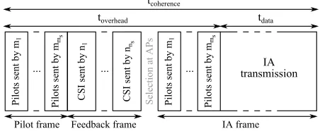
estimation at the receivers. In the feedback frame, the receivers send CSI back to the transmitters, which can then decide on node grouping, stream pairing, and mechanism selection. Finally, in the IA frame, all transmitters send the overlapping IA data. Note that we add again a non-overlapping pilot block in front to (a) detect if the channel has changed in between both frames, and (b) estimate carrier-frequency offset (CFO).
Channel quantization.After receiving the pilot frame, the receivers quantize the estimated CSI using a codebook to send it back. The codebook is known to both MSs and APs, and contains quantized CSI values. Hence, MSs do not need to send full CSI values back, but only the index of the codebook value which is most similar. The larger the codebook is, the more similar values can be found, but also the larger is the index in terms of bits, which has a direct impact on overhead. A codebook size of 64 is well suited for IA, as we have established in [6]. Hence, we use this value as a default size for our experiments. We also study the effects of bit errors in the feedback frame in order to assess its robustness. While we do not send feedback wirelessly, we do account for its overhead, and in [6] we show experimentally that the number of bit errors is small enough not to affect IA performance at all. For overhead calculations, we assume a1/2convolutional code to effectively protect feedback against external interference.
Time synchronization. IA requires that all APs start transmitting at exactly the same time. In our wireless access network scenario, we use the backbone to achieve synchro-nization between APs. At the receiver side, MSs need to detect the exact start of a frame. To this end, we use the 802.11 long preamble, which all transmitters send simultaneously. Still, for two consecutive frames the detected start may differ a few samples, introducing a phase offset. As a result, the precoding vectors based on the pilot frame are not valid for the IA frame. We correct this using the pilots preceding the IA frame.
Frequency synchronization. Slightly different oscillator frequencies at a receiver with respect to a sender cause CFO. This means that in our IA system each receiver would expe-rience a different CFO depending on the transmitter, which is hard to correct as transmissions overlap in the IA frame. We solve this using the backbone to share clocks among APs. Therefore, all signals experiencethe sameCFO, which can be easily corrected at the receivers using a pilot-aided technique.
AGC. We use Automatic Gain Control (AGC) to ensure that the overlapping signals in the IA frame do not saturate the receivers. The AGC is set for each frame using the 802.11 preamble, and all transmitters send it at the same time. Thus, the gains are set for the case of overlapping signals.
IA transmission
toverhead tdata
tcoherence
Pilot frame IA frame
Pilots sent
by m
1
Pilots sent
by m
ms
...
Pilots sent
by m
1
Pilots sent
by m
ms
...
CSI sent by n
1
CSI sent by n
n s
...
Feedback frame
Selection a
t APs
Fig. 2. Frame format for IA in a node subset of a wireless access network.
VI. EVALUATION
A. Testbed Setup
Hardware platform. Our testbed is based on WARP, which is an FPGA-based SDR developed at Rice University [18]. This allows us to experiment in settings similar to those of an 802.11 network, but with full control over the lower layers. We use the WARPLab Reference Design to evaluate our IA system flexibly in Matlab while still performing transmissions over-the-air. First, we calculate in Matlab the samples to be transmitted. These samples are then transferred via Ethernet to the sending WARP boards, which transmit them over the physical wireless medium. The receiving WARP boards sample the signal and send it back to Matlab. Note that in between the pilot and the IA frame, data is processed in Matlab, i.e., while not fully real-time due to the delay for transferring signals to and from Matlab, we do not process data offline, but online
and interactively. If implemented on the FPGA, our system
would run in real-time as our heuristics keep complexity low.
Coherence time.The aforementioned delays are not criti-cal for our testbed measurements since our setup is quasi-static and thus channels change slowly. This means that the CSI we obtain from the pilot frame is still up-to-date when we transmit the IA frame. Hence, while algorithms do not run in real-time on the FPGA, our testbed is perfectly suited for our purposes.
Throughput.We cannot measure throughput directly since the delays incurred by WAPRLab would strongly affect the result. Still, we define a “raw” throughput metric to capture the impact of (a) the BER, and (b) the overhead. This metric abstracts from data framing and error correction, but we use it to compare the fundamental performance of our schemes, except in Section VI-C7, where we do consider these issues. We take (a) into account by subtracting bit errors from received data, and (b) by including the overhead into the duration of the transmission. Also, the longer the IA frame is, the less weight the overhead carries. In turn, the coherence time gives the maximum length since pilots have to be updated as soon as the channels change. We consider an indoor environment, i.e., the coherence time is about 45 ms [6]. For calculations, we assume that the IA frame lasts the same as the coherence time, but in practice it would be divided into multiple smaller packets. Still, the key for overhead is that during the coherence time, CSI does not need to be measured again. Since WARPLab buffers are not large enough to send data for such a comparatively long time, we calculate the raw throughput “thp” by extrapolating our measurement as follows. We measure the correct bits received for a duration oftmeasure, calculate how many times tmeasure fits into tcoherence, subtract the time for transmitting
overhead and divide bytcoherence, as shown in Equation 7.
thp=(bitsTX−bitsERR)·
tcoherence−toverhead
tmeasure
tcoherence
(7)
are successful. We aim at maximizing throughput using IA at comparable BERs. In experiments VI-C1 to VI-C6 we discuss the interaction of both metrics for fixed modulation schemes to understand how our selections work. In experiment VI-C7 we then bring both metrics together using adaptive modulation.
Experiment setup. Our testbed consists of two WARPv3 boards, each with four radio interfaces. We use each radio as if it were an individual node, but all data sent and received is treated independently in Matlab. All radios on the first board act as transmitters, while all radios on the second board are receivers. Such a setup allows us to model 3×3 and
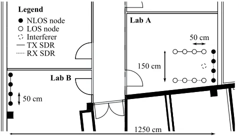
4 ×4 subsets with the aforementioned backbone, since all transmitters synchronize automatically, and share clocks. On the receiver side, having all nodes on one board is not required, but simplifies our testbed setup. If not stated otherwise, the two WARP boards are notsynchronized. In our experiments, we consider both a line-of-sight (LOS) and a non-line-of-sight (NLOS) scenario, as depicted in Figure 3. For some experiments we add an interferer to study the robustness of our IA schemes. For both LOS and NLOS, we keep SNRs in the range of typical indoor scenarios, that is, 20 to 30 dB.
If not stated otherwise, we use OFDM parameters equiv-alent to an 802.11g system, i.e., 18 MHz channels, 54 usable subcarriers, 312.5 KHz subcarrier spacing, and 12.5% cyclic prefix (CP). For experiments inspired by 802.11ac, we increase the number of subcarriers to 456, which in the standard corre-sponds to 160 MHz channels. Since WARP does not support such large bandwidths, we reduce the subcarrier spacing to 39 KHz, resulting in longer OFDM symbols. Still, this allows us to assess performance with a large number of subcarriers.
B. Network simulation
While we evaluate our IA system primarily in practice, we start with a simulation of a large and random topology which we cannot recreate in our testbed.
Setup.We assume a scenario with a large number of nodes in the same space, such as a conference room or a lobby. Our model consists of a square room with walls of length s and four APs, each placed in one corner. For each simulation run, we placenMSs at random locations and form subsets of size four, i.e., subsets include all APs, and four MSs chosen as in Section III-B2. For 3×3schemes, we only consider the first three APs. We assume a path loss exponent ofα= 2, Rayleigh channels and 70 dB SNR at a distance of 1 meter to the APs.
50 cm
150 cm Lab A
Lab B
1250 cm 50 cm
Legend NLOS node LOS node Interferer TX SDR RX SDR
Fig. 3. Node setup for practical experiments on SDRs.
Results. We focus on the results we cannot obtain in our testbed, namely, (a) random deployment of MSs in flexibly sized areas, and (b) a large number of nodes. Figure 4 depicts the gains in terms of throughput (c.f. Eq. 7) of IA compared to OFDM 4×4Optimized for increasing areas. The modulation scheme is 16-QAM, the number of nodes is fixed to 12, and we vary s from 5 to 80 meters. As expected, we observe an overall decline of gains with increasing room size, which is caused by nodes being on average further away from the APs and thus having lower SNRs. For the smallest considered area (s= 5), all algorithms achieve gains in between 25% and 30%. We do not reach the theoretical 33% maximum, because we include the feedback overhead with a codebook size of 64. The schemes using4×4subsets have slightly worse gains because they need to transmit CSI feedback of 16 links instead of only 9 links. However, this overhead pays off as soon as the room size increases and SNRs become lower—while the 3×3 schemes quickly degrade, the4×4ones maintain gains close to 25% up tos= 20due to selection. For larger room sizes, we observe that the throughput gain decreases more for IA+OFDM than for4×4IA. The BER is responsible for this behavior. For low SNRs, IA performs worse than OFDM w.r.t. the BER, that is, while IA may achieve larger gross throughput, its BER cancels out most of it in terms of raw throughput (Eq. 7). Hence, IA+OFDM gradually switches more subcarriers to OFDM in order to maintain a low BER, thus loosing throughput gain. In other words, IA+OFDM is able to dynamically adapt to channel conditions by transitioning individual subcarriers to OFDM when the SNR is too low.
In further experiments, we analyzed the impact of higher node densities on forming subsets. With more nodes per area, we expect to find better subsets since the probability of finding nodes with similar SNRs to all APs becomes larger (c.f. Section III-B2). Thus, we fix the area size and increase the number of nodes. As expected, the throughput decreases with the number of subsets, as we serve subsets in a time-division fashion. However, for each individual subset, the throughput is approximately constant, which means that we do not require a large number of nodes to find suitable subsets.
C. Testbed measurements
1) Plain IA: We first analyze how plain IA performs (i.e.,
without selection), and how the impact of practical issues is. Figure 5 depicts the THP gain and the BER in our LOS setup.
802.11g. First we focus on 802.11g, which is our default physical layer. We compare an idealized case, where we assume perfect CSI and synchronize both WARP boards to avoid CFO, with a realistic case where CSI is quantized, and
5x5 10x10 20x20 40x40 60x60 80x80
−10 0 10 20 30
AreaDsizeD[m]
GainD[%]
FixedDIAD3x3 Opt.DIAD3x3 Opt.DIAD4x4 Opt.DIA+OFDMD4x4
4−QAM 16−QAM 64−QAM 256−QAM 0.00
0.05 0.10 0.15
Modulationgorder
BitgErrorgRate
4−QAM 16−QAM 64−QAM 256−QAM
0 10 20 30
Gaing[5]
802.11ac,g estimatedgCFO, nogquantization 802.11ac,g estimatedgCFO, quantizedgCSI 802.11g,g nogCFO,g nogquantization 802.11g,g estimatedgCFO, quantizedgCSIg
Fig. 5. BER and THP gain for IA3×3Fixed over OFDM4×4Opt.
0 21 43 65 87 108 130 152
0.00 0.05 0.10 0.15 0.20 0.25 0.30
Time [Minutes]
BER
IA Fixed 3x3 IA Optimized 4x4
Fixed 3x3 OFDM
Fig. 6. BER over two and a half hours for 256-QAM in LOS setup.
CFO must be corrected. For perfect CSI, no feedback overhead is generated. The ideal case achieves close to 30% gain over OFDM4×4Optimized for 4-QAM. Since no selection is used, it degrades and incurs high BERs for higher modulations. The realistic case performs similarly, which means that we are able to cope successfully with CFO and CSI. However, gains are slightly lower due to the added feedback overhead.
802.11ac.Since we observed that we can cope with CFO, for the case inspired by 802.11ac we keep estimating it real-istically for both measurements. The first one assumes perfect CSI and achieves similar results to 802.11g, which shows that our IA system is also well suited for encoding a large number of subcarriers. For the second measurement—with quantized feedback—the gain drops despite similar BERs. The reason is that feedback overhead is much larger when sending CSI for 456 subcarriers than for 52 in 802.11g. Note that an 802.11ac system with 160 MHz channels would compensate for this.
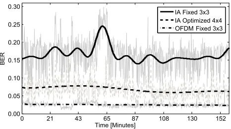
2) Time dependence: In our next experiment we compare
the behavior over time of IA3×3 Fixed with IA4×4 Opti-mized (Figures 6/7). In each measurement round all schemes are measured, i.e., they experience virtually the same CSI for each time in Figures 6/7. We fit curves on our measurements to highlight their behavior. In both figures, IA4×4Opt. is clearly more stable than plain IA, since itadaptsto changing channel conditions, while plain IA cannot avoid CSI fluctuations.
In particular, Figure 6 depicts the BER during 2.5 hours for 256-QAM. At about minute 65, a change in channel quality increases the BER for plain IA for about 10 minutes. Meanwhile, IA 4×4 Optimized absorbs the CSI change by automatically transitioning to a suitable node/stream allocation, and is not affected at all. Figure 7 depicts the throughput for six hours using 16-QAM, which is less prone to errors. Thus,
0 1 2 3 4 5 6
68 72 76 80
Timez[hours]
Throughputz[mbps]
IAz3x3zFixed IAz4x4zOptimized
Fig. 7. THP over six hours during daytime for 16-QAM in LOS setup.
4−QAM 16−QAM 64−QAM 256−QAM 0
10 20 30
Through
put gain [%]
Fixed IA 3x3 Opt. IA 3x3 Opt. IA 4x4
IA 3x3 is limited to using nodes 1 to 3
T1
R1 R2 R3 R4
T2
T3
T4
Fig. 8. THP gain placing one transmitter (T3) far away from the receivers.
both IA4×4Optimized and IA3×3Fixed perform similarly. However, note that IA 3 ×3 Fixed continuously fluctuates around the average value while IA4×4 Optimized is stable.
3) Node selection: We now investigate scenarios where the
selection algorithms benefit most, starting with node selection. To highlight its operation, we place the third transmitter of the LOS setup further away from the receivers, as depicted in Figure 8. The key is that 3×3 algorithms are forced to use the far away node T3, while 4×4 schemes can resort
toT4, which is much closer and thus has better channels. As
expected, the results in Figure 8 show that both IA3×3Fixed and Optimized perform significantly worse than IA4×4. Note that for 4-QAM IA 3×3Opt. still achieves good gains, since its stream selection improves performance just enough for 4-QAM to work, but not enough for higher modulations.
4) Mechanism selection: Next, we show how mechanism
selection improves transmission in terms of BER for heteroge-neous scenarios. To this end, we use our NLOS setup and place one transmitter closer to the receivers, as illustrated in Fig. 9. When switching from NLOS to the “closer” setup, IA 4×4
Opt. experiences no improvement, since it involves at least three nodes, and is limited by the SNRs of the far away ones. IA+OFDM instead cuts down the BER tohalf its value, since it can allocate individual OFDM subcarriers to the node with better SNR. It trades throughput for BER, which is essential if the channel code in use cannot cope with large BERs.
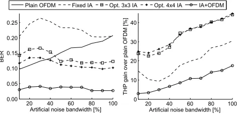
5) External interference: In what follows, we investigate
the robustness of selections when adapting to external interfer-ence. We generate artificial noise on an increasing percentage of subcarriers using the interferer in Figure 3. We set low transmission gains to fit the setup. Thus, nodes on the right side of the LOS setup are more strongly affected than nodes on the left. The results are shown in Figure 10. OFDM 4×4
IA+OFDM is not affected, since it chooses the left3×3group out of the 4×4subset to adapt to the interferer on the right. For the IA algorithms without mechanism selection (dashed lines), we observe a common trend. For a noise bandwidth up to 30%, the BER rises, but beyond 30% it falls again. The reason is that subcarrier combinations are evenly distributed over the available bandwidth (c.f. Section III-B1). Hence, even narrow noise bandwidths quickly affect at least one subcarrier in each combination, causing a steep initial rise of the BER. The subsequent decline beyond 30% is due to the increasing distribution of noise power. Our interference signal has the same power for all noise bandwidths, which means that for narrow bandwidths, a large noise affects only a few subcarriers, while a smaller noise affects many subcarriers for large bandwidths. Thus, we conclude that IA can cope better with small noise affecting all subcarriers in a combination than with large noise affecting only one subcarrier. In other words, the noisiest subcarrier determines the performance of IA. The optimized IA algorithms stabilize already at 50% noise bandwidth since they can circumvent noisy links by selection. For OFDM, noise power is also constant, but the BER improvement due to less noise per subcarrier is smaller than the degradation due to noise affecting more subcarriers. Regarding throughput gain, all mechanisms tend to improve with increasing noise due to the baseline degrading linearly.
6) NLOS setup: We now investigate IA performance in
our NLOS setup. The results are depicted in Figure 11. For low modulation schemes all algorithms achieve significant gains. However, while plain IA 3×3Fixed degrades quickly for increasing modulations, our selection algorithms enable optimized IA to provide gains above 15% even for 256-QAM. When switching from 64-QAM to 256-QAM, IA+OFDM transitions to using OFDM on most subcarrier combinations, thus loosing gain but achieving BERs comparable to OFDM
4×4 Optimized. We conclude that IA in NLOS scenarios is feasible and benefits from node/stream/mechanism selection.
7) Adaptive modulation: In previous experiments we study
the IA gain for individual modulation schemes. Next, we analyze its behavior for adaptive modulation. Since IA has higher SNR requirements than plain OFDM, IA typically has larger BER for a given modulation. Hence, this raises the question whether for a given BER, plain OFDM could simply switch to a higher modulation than IA and thus achieve higher throughput. To understand this issue, we analyze a system where APs adaptively choose for each frame the modulation and technique (IA or OFDM) that provides best throughput.
NLOS Closer 0
5 10 15
Through
put gain [%]
Optimized IA 4x4 Optimized IA+OFDM 4x4
NLOS Closer 0.00
0.05 0.10 0.15 0.20 0.25
BER
Closer setup: all Tx
are far exept one R1 R2 R3 R4
T1 T2 T3
T4
Fig. 9. THP gain over plain OFDM and BER in the “closer” setup.
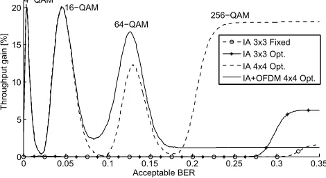
Similarly to a real-world system, APs aim at achieving a certain acceptable BER for each frame. The acceptable BER may be the error correction capability of the code in use, or the BER allowed by a loss-tolerant stream such as video. In Figure 12, we show performance for a range of acceptable BER values, without limiting them to a specific coding scheme or stream type. For this experiment, we use an overnight measure-ment (9.5 hours) in our NLOS scenario. Hence, the average SNR is constant and provided by our setup. In particular, we continuously measure all our schemes for all M-QAM modulation orders we consider, i.e.,M∈[4,16,64,256]. Then, for each acceptable BER value, we find the best modulation and technique (IA or OFDM). We compare results to a baseline which always uses OFDM, but still adapts modulation, i.e., we do consider the case where our system and the baseline are usingdifferentmodulation orders. In Figure 12, the gain peaks occur when the acceptable BER is larger than required for a certain modulation order in plain OFDM, but not enough for OFDM to switch to the next modulation. These are the margins where IA pays off, since this “excess” of the acceptable BER absorbs the higher SNR requirements of IA. For instance, such margins naturally occur for error correction codes. This happens because practical protocols usually provide a fixed set of codes, among which it is possible to choose, and thus the code often corrects more errors than actually needed. Since each modulation order is feasible for a different range of acceptable BERs, we observe multiple peaks in Figure 12. Note that only 4 × 4 algorithms achieve gain, while the aforementioned margins are too small for all other IA schemes. This showcases how selection not only enables IA but also makes it profitable in a realistic setting. For the 64-QAM peak, IA+OFDM achieves even better results than IA4×4, because it uses IA only on good subcarriers. Also, it stabilizes at a rather low gain value, since it transitions most of its subcarriers to OFDM for large BERs. This translates into no increased DOF.
VII. DISCUSSION
While we consider particular cases in our testbed evalua-tion, our simulations with random node locations and variable SNRs provide equivalent results. Hence, we conclude that our testbed experiments are representative and can be generalized tolarger networks. The subset sizeis critical for feasibility, since full CSI of each subset link is required and the number of possible node selections explodes in large subsets. We expect the latter to be the constraining factor, since in our experiments overhead has a limited impact. Still, larger subsets increase the probability of finding good selections. In our testbed, a
Artificial noise bandwidth [0]
BER
20 40 60 80 100 0.00
0.05 0.10 0.15 0.20 0.25
PlainHOFDM Fixed IA Opt. 3x3 IA Opt. 4x4 IA IA5OFDM
20 40 60 80 100
0 10 20 30 40
Artificial noise bandwidthH[0]
THPHgai
nHoverHpla
inHOFDMH[0]
QAM
4−QAM 16−QAM 64−QAM 256−
Gain [
%]
Fixed IA 3x3 Opt. IA 3x3
IA 4x4 IA+OFDM 4x4 30
25
20
15
10
5
0
Fig. 11. THP gain compared to OFDM4×4Optimized in our NLOS setup.
Throu
ghputEgain
E[D]
0 0.05 0.1 0.15 0.2 0.25 0.3 0.35
0 5 10 15 20
IAE3x3EFixed IAE3x3EOpt. IAE4x4EOpt. IA+OFDME4x4EOpt. 4−QAM
16−QAM
256−QAM 64−QAM
AcceptableEBER
Fig. 12. Throughput gain compared to plain OFDM with adaptive modulation.
subset size of 4×4is an operable trade-off. Despite the high SNR requirements of IA, we show that it provides gains with realistic adaptive modulation. The gain is directly related to the acceptable BER, which in turn depends on the coding scheme in use, the type of data sent, and ultimately on the application. Hence, cross-layer optimizations to fully exploit the benefits of IA are possible, but we consider this to be out of scope of this paper. Also, while we select resources based on a physical layer metric, our approach opens the door to metrics that include upper-layer requirements. Finally, our selection algorithms can transition from one resource allocation to another in order to adapt to changing channel conditions on a subcarrier-wise basis. We believe that this is key to enable IA, as adaptation is crucial in a wireless environment.
VIII. CONCLUSION
We propose an architecture for a wireless access network based on Interference Alignment (IA) at the physical layer. To this end, we deal with the practical issues of such a system. Still, the key challenge of IA lies in the high SNRs required. While an indoor wireless network might provide such SNRs, channel quality is typically heterogeneous and variable. Hence, selecting which nodes participate in IA using which resources is crucial. We contribute three selection algorithms to choose groups of nodes on top of which to operate, stream pairs within each group, and alternative mechanisms in case of strongly impaired channels. Selection decisions are based on an EVM metric which can be calculated for each possible selection. We implement our approach on a software-defined radio (SDR) and conduct experiments in heterogeneous scenarios. Moreover, we perform simulations to validate our results in random networks. We achieve up to 30% gain compared to plain OFDM. Future work includes choosing optimized IA precoding vectors and investigating practical Sphere Decoding.
REFERENCES
[1] S. Kumar, D. Cifuentes, S. Gollakota, and D. Katabi, “Bringing cross-layer MIMO to today’s wireless LANs,” in Proc. ACM SIGCOMM, 2013.
[2] H. S. Rahul, S. Kumar, and D. Katabi, “JMB: scaling wireless capacity with user demands,” inProc. ACM SIGCOMM, 2012.
[3] S. Katti, D. Katabi, H. Balakrishnan, and M. Medard, “Symbol-level network coding for wireless mesh networks,” inProc. ACM SIGCOMM, 2008.
[4] V. R. Cadambe and S. A. Jafar, “Interference alignment and degrees of freedom of the k-user interference channel,”IEEE Trans. on Information Theory, vol. 54, no. 8, 2008.
[5] P. Razaghi and G. Caire, “Interference alignment, carrier pairing, and lattice decoding,” inProc. IEEE International Symposium on Wireless Communication Systems, 2011.
[6] A. Loch, T. Nitsche, A. Kuehne, M. Hollick, J. Widmer, and A. Klein, “Practical challenges of IA in frequency,” TU Darmstadt, SEEMOO, Tech. Rep., 2013. [Online]. Available: http://www.seemoo.de/ia [7] M. Shen, A. Host-Madsen, and J. Vidal, “An improved interference
alignment scheme for frequency selective channels,” in Proc. IEEE International Symposium on Information Theory, 2008.
[8] V. R. Cadambe and S. A. Jafar, “Interference alignment and spatial degrees of freedom for the k user interference channel,” inProc. IEEE International Conference on Communications (ICC 2008), May 2008. [9] S. Peters and R. Heath, “Interference alignment via alternating mini-mization,” inProc. IEEE International Conf. Acoustics, Speech Signal Processing, 2009.
[10] L. E. Li, R. Alimi, D. Shen, H. Viswanathan, and Y. R. Yang, “A general algorithm for interference alignment and cancellation in wireless networks,” in Proc. of Conference on Information communications (INFOCOM), 2010.
[11] T. Gou, C. Wang, and S. Jafar, “Aiming perfectly in the dark-blind interference alignment through staggered antenna switching,” inProc. IEEE Global Telecommunications Conference (GLOBECOM), 2010. [12] S. A. Jafar, “Blind interference alignment,”IEEE Journal on Selected
Areas in Communications, vol. 6, no. 3, June 2012.
[13] G. Bresler, A. Parekh, and D. Tse, “The approximate capacity of the many-to-one and one-to-many gaussian interference channels,” IEEE Trans. Inf. Theory, vol. 56, no. 9, 2010.
[14] O. Elayach, S. W. Peters, and R. W. H. Jr., “The practical challenges of interference alignment,”IEEE Wireless Communications, pp. 35–42, Feb. 2013.
[15] D. R. O. Gonzalez, I. Santamaria, J. A. Garcia-Naya, and L. Castedo, “Experimental validation of interference alignment techniques using a multiuser MIMO testbed,” inProc. Workshop on Smart Antennas, 2011. [16] S. Gollakota, S. D. Perli, and D. Katabi, “Interference alignment and
cancellation,” inProc. SIGCOMM, Aug. 2009.
[17] K. Miller, A. Sanne, K. Srinivasan, and S. Vishwanath, “Enabling real-time interference alignment: promises and challenges,” inProc. ACM International Symposium on Mobile Ad Hoc Networking and Computing (MobiHoc), 2012.
[18] “Rice Univ. WARP Project.” [Online]. Available: http://warp.rice.edu [19] H. V. Balan, R. Rogalin, A. Michaloliakos, K. Psounis, and G. Caire,
“Achieving high data rates in a distributed MIMO system,” in Proc. MobiCom, 2012.
[20] J. W. Massey, J. Starr, S. Lee, D. Lee, A. Gerstlauer, and R. W. H. Jr., “Implementation of a real-time wireless interference alignment network,” in Proc. Asilomar Conference on Signals, Systems and Computers (ASCSSC), 2012.
[21] M. Shena, X. Lianga, C. Zhaoa, and Z. Ding, “Best-effort interference alignment in OFDM systems with finite SNR,” inProc. International Conference on Communications (ICC), 2011.
[22] R. Brandt, H. Asplund, and M. Bengtsson, “Interference alignment in frequency - a measurement based performance analysis,” in Proc. International Conference on Systems, Signals and Image Processing (IWSSIP), 2012.