Article
1
Image Features Based on Characteristic Curves and
2
Local Binary Patterns for Automated HER2 Scoring
3
Ramakrishnan Mukundan 1,*
4
1 Department of Computer Science and Software Engineering, University of Canterbury, Christchurch,
5
New Zealand; [email protected]
6
* Correspondence: [email protected]; Tel.: +64-3-3692201
7
8
Abstract: This paper presents novel feature descriptors and classification algorithms for
9
automated scoring of HER2 in Whole Slide Images (WSI) of breast cancer histology slides. Since a
10
large amount of processing is involved in analyzing WSI images, the primary design goal has been
11
to keep the computational complexity to the minimum possible level and to use simple, yet robust
12
feature descriptors that can provide accurate classification of the slides. We propose two types of
13
feature descriptors that encode important information about staining patterns and the percentage of
14
staining present in ImmunoHistoChemistry (IHC) stained slides. The first descriptor is called a
15
characteristic curve which is a smooth non-increasing curve that represents the variation of
16
percentage of staining with saturation levels. The second new descriptor introduced in this paper is
17
an LBP feature curve which is also a non-increasing smooth curve that represents the local texture of
18
the staining patterns. Both descriptors show excellent interclass variance and intraclass correlation,
19
and are suitable for the design of automatic HER2 classification algorithms. This paper gives the
20
detailed theoretical aspects of the feature descriptors and also provides experimental results and
21
comparative analysis.
22
Keywords: medical image classification; local binary patterns; characteristic curves; whole slide
23
image processing; automated HER2 scoring
24
25
26
1. Introduction
27
The most commonly used method for breast cancer grading is the ImmunoHistoChemistry
28
(IHC) test which is a staining process performed on biopsy samples of breast cancer tissues [1]. The
29
IHC stained slides are normally observed under a microscope by pathologists to determine the level
30
of over-expression of Human Epidermal Growth factor Receptor 2 (HER2) protein in cancer cells.
31
The tissue sample is then assigned a HER2 score of 0 to 3+ representing the grade of cancer present
32
in the sample [2]. Manual grading and annotations of breast cancer slides are time consuming,
33
and there are huge maintenance costs associated with collecting, archiving, and transporting tissue
34
specimens. It is also well documented that manual grading can have significant variability in
35
pathologist assessments due to the subjective process of determining the intensity and uniformity of
36
staining in the presence of variable staining patterns and heterogeneity of tumor grade [3].
37
Automated methods can also suffer from errors due to inaccuracies in the training algorithm and its
38
inability to segment faint and complex tissue structures [4].
39
In the rapidly growing field of digital pathology, several Whole Slide Image (WSI) processing
40
algorithms are currently being developed as diagnostic tools to help pathologists in the assessment
41
of disease patterns [5]. WSIs have a pyramidal structure to enable optimized viewing across multiple
42
magnification levels, and they provide a high resolution overview of the entire slide [5,6]. Typically
43
at 40x magnification, the images have a resolution of approximately 0.25 microns per pixel. At this
44
resolution, a slide region of size 15mm x 15mm could correspond to 60,000 x 60,000 pixels. WSIs
45
were originally used as a computer aided digital microscopy tool, where pathologists could view
46
different parts of a sample at different magnifications to improve the accuracy of their scores [3].
47
Powerful computational algorithms are being developed to automatically extract features related to
48
cytological and protein structures in the image for accurately quantifying biomarkers like HER2 [7].
49
In [8], the authors used adaptive thresholding and watershed algorithm for cell segmentation.
50
Recently, an online contest was organized by the University of Warwick in conjunction with the
51
UK/Ireland Pathology Society annual meeting 2016, with the aim of advancing research in the field
52
of automated HER2 scoring algorithms [9]. This contest was the primary motivation for our research
53
work presented in this paper. Our algorithm (registered with team name UC-CSSE-CGIP)
54
performed exceedingly well in the contest, obtaining the second best points score of 390 out of 420
55
and the overall seventh position in the combined leader board [10]. The teams that were on the top of
56
the leader board, including our team, were invited to submit a very brief (one paragraph) summary
57
of the algorithms used for inclusion in a journal paper prepared by the contest organizers [11].
58
WSIs contain voluminous amounts of data. One of the primary design goals has been to keep
59
the computational complexity to the minimum possible level and to develop an efficient method that
60
can process relevant tiles of an input WSI image quickly and classify the image into one of the four
61
classes corresponding to the four HER2 scores. The second design goal was to have a feature set
62
whose correlation to the percentage of membrane staining in the given sample could be easily
63
visualized and interpreted by pathologists. The third design goal was to reduce the amount of
64
information redundancy in the feature set by extracting a minimal set of characteristic features that
65
would adequately represent the staining pattern and the percentage of staining. This paper presents
66
two types of feature descriptors that have shown excellent intraclass correlation and interclass
67
variance in our experimental analysis involving a large collection of WSI images. The first descriptor
68
is called characteristic curves and they represent the variation of the percentage of staining in an
69
image tile with saturation levels of the staining colour. The second descriptor is based on local
70
binary patterns [12], and they encode information about the local texture variation in the image with
71
saturation levels. The paper provides a detailed description of the WSI processing stages,
72
development and selection of features, and the experimental analysis performed. We hope that the
73
methods presented in this paper will contribute significantly to the development of faster and
74
accurate automatic HER2 scoring techniques in the area of breast cancer histopathology.
75
The paper is organized as follows: The next section gives a description of the dataset used, an
76
outline of HER2 assessment scheme and an overview of the stages of the processing pipeline.
77
Section 3 provides an introduction to a novel set of features called characteristic curves and
78
discusses their computational aspects and properties. Section 4 gives an overview of local binary
79
patterns, their computation, and introduces another set of feature descriptors called LBP feature
80
curves. Section 5 gives a brief description of a classification algorithm using the proposed feature
81
descriptors for classifying histopathological images based on their HER2 scores. and Section 5
82
presents experimental results and comparative analysis. Section 6 presents experimental results
83
and analysis. Section 7 concludes the paper with a summary of important aspects of the proposed
84
features and outlines future research directions.
85
2. Materials and Methods
86
2.1 HER2 Assessment
87
The amplification of HER2 genes and correspondingly the over-expression of HER2 protein
88
receptors play an important role in the development of breast cancer. The assessment of HER2
89
protein over-expression is done using the ImmunoHistoChemistry (IHC) test based on the
90
percentage of membrane staining observed in tumor cells as well as the intensity of staining [2]. The
91
mapping between the level of membrane staining and the reported HER2 score is shown in Table 1.
92
Table 1. Correlation between the intensity and percentage of membrane staining and the assigned
94
HER2 scores [2].
95
HER2 Score Assessment Staining Pattern
0 Negative No staining is observed, or membrane staining is observed in less than 10% of tumor cells
1+ Negative A faint/barely perceptible membrane staining is detected in greater than 10% of tumor cells. The cells exhibit incomplete membrane staining.
2+ Weakly Positive
A weak to moderate membrane staining is observed in greater than 10% of tumor cells.
3+ Positive A strong complete membrane staining is observed in greater than 10% of tumor cells.
96
A few sample tiles from WSI images of IHC stained slides are given in Figure. 1 along with the
97
HER2 scores to show the variations of the scores with the level of membrane staining seen in the
98
images.
99
100
HER2 Score = 0 HER2 Score = 1+ HER2 Score = 2+ HER2 Score = 3+
Figure 1. WSI tiles showing different levels of staining and corresponding HER2 scores.
101
2.2 Dataset
102
The dataset used in this research work was provided by the University of Warwick as part of
103
the online HER2 scoring contest [9]. Permission was granted by the contest organizers to
104
participating teams for the use of the dataset for research and academic purposes. The dataset
105
consisted of a total of 172 whole slide images in Nano-zoomer Digital Pathology (NDPI) format.
106
These WSIs were extracted from 86 cases of patients with invasive breast carcinomas [11]. For each
107
case, WSIs of both Hematoxylin and Eosin (H&E) stained and IHC stained slides were provided.
108
There were two HER2 scoring contests, and the number of WSIs provided for training and testing
109
the classification algorithm is given in Table 2.
110
Table 2. Number of WSIs provided for training and testing the classification algorithm.
111
Training Set Test Set
Ground Truth HER2 Score Number of WSIs Contest-1
No. of WSIs
Contest-2 No. of WSIs
0 13 28 6
1+ 13 2+ 13 3+ 13 Total: 52
112
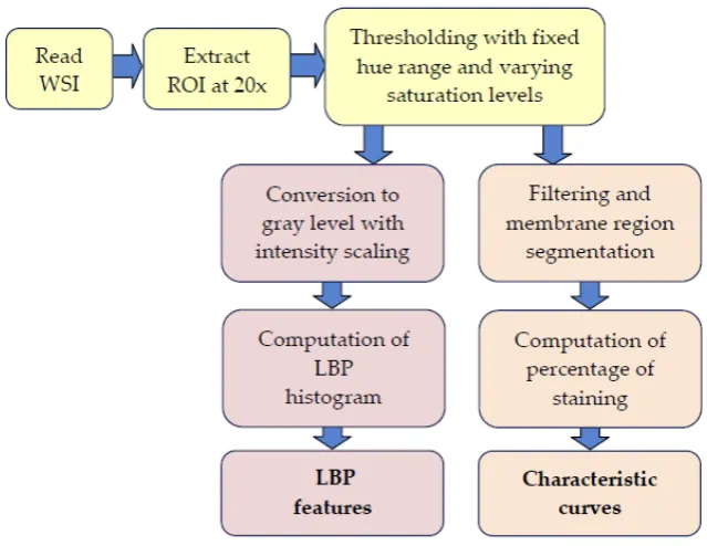
2.3 Processing Stages
113
Various stages of the processing pipeline are shown in Figure 2. We used the OpenSlide API
114
of the imaged tissue is extracted from the middle segment of the image. Rectangular tiles of size
116
1800 x 1200 pixels at 20x magnificaiton that contain at most 20% background pixels are then created
117
and used as inputs for the method that computes LBP features and characteristic curves. At least
118
six tiles at randomly selected locations within the ROI are generated for each WSI. The remaining
119
part of the pipeline thresholds the input tiles and computes the LBP features and also the percentage
120
of staining in the tissue sample to obtain the characteristic curves. These steps are detailed in the
121
following sections.
122
123
124
Figure 2. Processing stages in the extraction of characteristic curves and LBP features
125
3. Characteristic Curves
126
Curve based automated analysis of immunohistochemical images have been tried in the past
127
with limited success [14]. In this section, we introduce a novel feature vector called a characteristic
128
curve. An important parameter in HER2 assessment is the percentage of membrane staining
129
perceived in an image segment. Assuming that we can compute the percentage of membranes
130
stained in a particular colour range (this computation will be discussed in detail below), we can
131
analyse the variations in this percentage value with respect to changes in the colour saturation
132
threshold. Specifically, if [h, s, v] represent the stain colour components in HSV space, and if p(slow)
133
denotes the pecentage of staining with colour in the range given by the following inequalities:
134
h1 ≤ h < h2 s > slow
v1≤ v < v2 , (1)
then, the variation of p(slow) plotted against slow gives the characteristic curve (or the
135
percentage-saturation curve) of the image. In Equation 1, [h1, h2] denote fixed hue thresholds
136
specifying allowable variations in the hue value, and similarly [v1, v2] denote value thresholds.
137
Since we specify only the lower bound for saturation, progressively increasing slow, typically from 0.1
138
to 0.5, produces a non-increasing characteristic curve (Figure 3).
139
The base components of the stain colour [h, s, v] are computed using the training set where the
140
given percentage of staining is above 80%. While computing the percentage of staining for the test
141
(or cross-validation) sets, it is important to eliminate not only the background region but also other
142
These regions can be segmented using colour (nuclei are stained in a distinctly different colour) or
144
using a distance measure evaluated in colour space over a neighborhood mask around each pixel
145
(for identifying regions of nearly constant colour value)
146
147
148
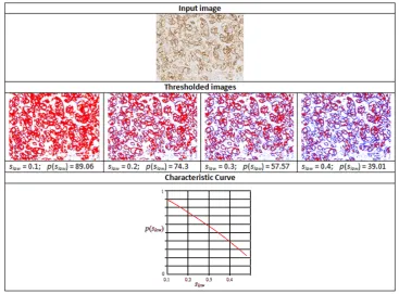
Figure 3. Intermediate stages in the generation of a characteristic curve.
149
Figure 3 shows thresholded images with stained regions in red colour as the value of slow is
150
increased from 0.1 to 0.4. The resulting characteristic curve is also shown. The characteristics curves
151
have the property that they are always monotonically decreasing smooth curves. They allow
152
accurate polynomial approximations using cubic curves. The shape of the curve can be directly
153
matched with the staining patterns given in the HER2 assessment guidelines (Table 1) for a
154
straightforward interpretation of the derived score (Figure 4). For example, the characteristic curve
155
always lies below the 10% threshold when the score is 0, and only a small initial segment of the curve
156
lies above the 10% mark when the score is 1. If the score is 3+, the curve lies completely above the
157
30% mark showing a strong and complete membrane staining. As seen in Figure 4, the curve passes
158
through a much wider range of values of percentage staining when the score is 2+.
159
160
161
The properties of the characteristic curve outlined above, particularly the fact that the curve is
163
non-increasing, can be used for developing a naive rule-based classification algorithm as follows.
164
• If z0 ( = p(0.1)) < 10%, then the whole curve lies below 10%, and the score is 0
165
• Else if zn−1 ( = p(0.5)) > 30%, then the whole curve lies above 30%, and the score is 3+
166
• Else if 10% ≤ z0 ( = p(0.1)) < 40% and p(0.2) < 15%, the score is 1+
167
• Else if p(0.4) < 15%, then the score is 2+
168
• Else, the score is 3+
169
The rules were formed by analyzing the shapes of characteristic curves for several image tiles
170
with ground truth values of HER2 scores assigned by pathologists. Note that for the above simple
171
classification algorithm, we sample the curve at only four key points p(0.1), p(0.2), p(0.4), and
172
p(0.5). We outlined the rule based algorithm here primarily to show the feature representation
173
capability of the characteristic curves.
174
4. Local Binary Patterns
175
4.1 LBP Computation
176
Local binary patterns (LBP) are powerful feature descriptors used for texture analysis and
177
classification [12]. The binary pattern is derived by comparing the intensity at each pixel with its
178
eight neighbors and encoding the information in an 8-bit integer value. This encoding can be viewed
179
as a transformation of the input image into an LBP image as shown in Figure 9. The histogram of the
180
LBP image is generally used for texture classification. In the area of medical image analysis, LBP
181
methods have been successfully used in characterizing disease patterns [15-17] and automated
182
diagnosis [18]. Local binary patterns have also been used for analyzing histopathological images and
183
detecting mitotic cells [19,20]. Several variants of LBP features such as hierarchical LPB have also
184
been proposed for specific applications like retinal vein occlusion recognition [21].
185
186
187
Figure 5. The intermediate steps in the computation of the LBP histogram of an image.
188
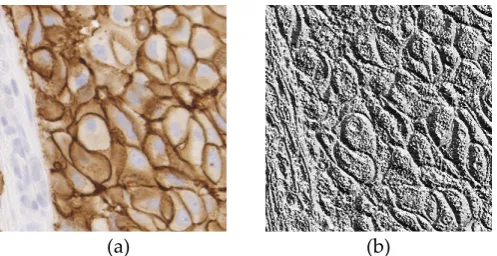
As an example, an input image and its LBP image are shown in Figure 6.
189
190
(a) (b)
192
As discussed in Section 3, we first obtain a thresholded image using a hue range [h1, h2] and
193
saturation values with s > slow. The pixels passing the threshold test are converted to gray level by
194
mapping h1 to 0 and h2 to 255. This gray level image is used as the input for LBP computation. The
195
LBP histogram of such images contain predominant features that represent the texture
characteris-196
tics of the staining patterns.
197
4.2 LBP Feature Curves
198
An LBP histogram is shown in Figure 7. The important LBP features are highlighted based on
199
their magnitudes. The LBP histogram contains 256 values Li , i = 0…255. We propose the
fol-200
lowing set of five LBP features for classification:
201
V = {L2, L32, L128, L223, L253} (2)
202
203
204
Figure 7. An LBP histogram showing the predominant feature components.
205
Each feature in the above set can generate a feature curve as detailed below. Consider one of the
206
LBP feature components, say L32. When the input image's saturation threshold slow is varied from 0.1
207
to 0.4 as discussed in Section 3, we get the corresponding variation in L32. This variation in the values
208
of L32 shows a non-increasing trend very similar to that of the characteristic curve.
209
210
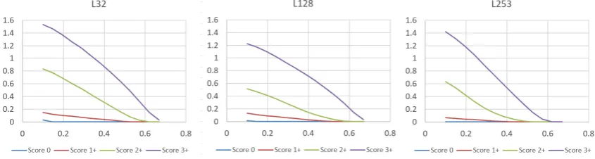
211
Figure 8. Normalized LBP feature curves for L32, L128, L253 showing the variations of their magnitudes
212
when the values of the saturation threshold slow are varied from 0.1 to 0.8 (x-axis).
213
The values of the LBP feature curves are normalized to remove any variations due to changes in
214
image size as follows:
215
where, w, h denote the width and the height of the input image. The variations of three LBP
216
feature components L′32, L′128, and L′253 with the saturation threshold for images with HER2 scores 0,
217
1+, 2+ and 3+ are shown in Figure 8.
218
The LBP feature curves bear similarity with characteristic curves in that they do not contain
219
high frequency variations and are non-increasing. Further, as can be seen in Figure 8, LBP feature
220
curves also show excellent discriminating power between the four HER2 classes, making them
221
suitable for use as feature vectors in classification algorithms.
222
5. HER2 Classification and Scoring
223
In this section, we outline a ‘one-vs-all’ multi-class classification algorithm using logistic
re-224
gression [22]. Logistic regression was chosen to minimize the computational complexity. Higher
225
order methods such as neural networks could also be designed with the use of the feature vectors
226
proposed in this paper. For a given training example with index j, the points sampled along its
227
characteristic curve or LBP feature curve xi(j) = p(si), i = 1..n, j = 1..m are used as features. The class
228
labels are denoted by yj∈[0, 3], j = 1..m. We denote the feature matrix by X∈ℜm×(n+1), the output
229
vector of labels by Y∈ℜm×1, and the classifier parameter vector for each class by θk ∈ℜ(n+1)×1, k = 1..4.
230
Here, class-1 corresponds to the set of training examples with HER2 score 1+, class-2 with HER2
231
score 2+, class-3 with HER2 score 3+ and class-4 with HER2 score 0. We then have the following
232
equations for the hypothesis functions H, the cost function and the gradient functions:
233
H = g(Xθk) (3)
where, H∈ℜm×1, and g() denotes the sigmoid function. The cost function J(θk) is then given by
234
(
log( ) (1 ) log(1 ))
1 )
( Y H Y H
m
J T T
k =− − − −
θ (4)
and the gradient function vector J′(θk) is defined as
235
(
( ))
1 )
( X H Y
m
J T
k =− −
′ θ , k = 1..4. (5)
For prediction, the points xi on the characteristic curve or the LBP feature curve of a given
236
sample are combined with the trained values of class parameters θk for each class k = 1..4, and the
237
class that gives the maximum value for g(xi′θk) is chosen. In the next section, we provide the result
238
of classification experiments using the above methods.
239
6. Experimental Results and Analysis
240
We used features computed from 52 WSIs with 3 tiles at 20x from each image (comprising of
241
156 images) and their ground truth values as the training data. Another set of 3 tiles from each of the
242
52 cases formed the cross-validation set. Out of the total of 156 image tiles in the cross-validation
243
set, 39 belonged to each of the four classes corresponding to four HER2 scores. For generating
fea-244
ture vectors for classification using logistic regression, it was found that a step size of 0.02 for the
245
saturation threshold would provide an adequate number of 20 points (features) within the
satura-246
tion range slow∈ [0.1, 0.5]. The feature matrix X in Equation 3 therefore had the dimension 156×20.
247
The gradient descent algorithm used 100 iterations to converge to the solution with a learning rate of
248
250
Figure 9. Convergence of the cost functions of the four-class logistic regression algorithm.
251
Figure 9 gives a sample plot of cost function values for each of the four classes, where the
252
characteristic curves consisting of 20 features for each sample were used as feature vectors. The
253
confusion matrix in Table 3 summarizes the results for each class and gives the overall accuracy
254
achieved.
255
Table 3. Confusion matrix for the multi-class logistic regression algorithm
256
Predicted Accuracy = 88.46%
0 1+ 2+ 3+ Precision Recall
Actual
0 37 2 0 0 0.86 0.95
1+ 6 29 4 0 0.83 0.74
2+ 0 4 34 1 0.87 0.87
3+ 0 0 1 38 0.97 0.97
257
The smoothness and monotonically decreasing properties of the characteristic curve can be
ef-258
fectively made use of in reducing the dimensionality of the features in the logistic regression
algo-259
rithm. As in the case of the rule based classification method, we can sample the curve at only four
260
key points p(0.1), p(0.2), p(0.4), and p(0.5), and also use the slope information at those points
261
p′(0.1), p′(0.2), p′(0.4), and p′(0.5) to get a feature vector of size 8 instead of 20. The cost functions
262
converge to almost similar values with only a slight increase in the magnitudes. The confusion
ma-263
trix obtained by running the algorithm with the reduced set of features of the characteristic curve is
264
shown in Table 4.
265
Table 4. Confusion matrix for the multi-class logistic regression algorithm with the reduced feature
266
set.
267
Predicted Accuracy = 83.3%
0 1+ 2+ 3+ Precision Recall
Actual
0 37 2 0 0 0.80 0.95
1+ 8 24 7 0 0.75 0.61
2+ 1 6 31 1 0.79 0.79
3+ 0 0 1 38 0.97 0.97
268
As seen in Table 4, reducing the dimensionality of the feature set from 20 to 8 only affected the
269
recall rates of classes 1 and 2.
270
Experimental analysis using LBP feature curves also gave reasonably good levels of accuracy.
271
Only one LBP feature curve selected from the set in Equation 2 was used in our analysis, and the
272
feature vector consisted of 20 sample points along the curve. We give below the results for the
fea-273
Table 5. Confusion matrix for the multi-class logistic regression algorithm with the LBP feature
275
vector L32.
276
Predicted Accuracy = 87.18%
0 1+ 2+ 3+ Precision Recall
Actual
0 38 1 0 0 0.84 0.97
1+ 6 27 6 0 0.82 0.69
2+ 1 5 32 1 0.84 0.82
3+ 0 0 0 39 0.98 1.00
277
278
The texture characteristics represented by LBP features were useful in resolving some of the
279
ambiguous cases for scores 0 and 3+ where the texture features are highly distinguishable, providing
280
higher recall rates for those two scores. The LBP features also gave higher false positives for score 2+.
281
Overall, logistic regression with 20 feature points computed from the characteristic curves gave the
282
highest accuracy of 88.5%.
283
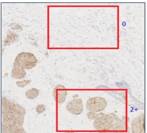
Analysing the staining patterns in tiles that were wrongly classified revealed a common
prob-284
lem in the automatic extraction of tiles from WSIs. Some of the samples with scores 1+ and 2+ had
285
large tissue regions without any staining. The example shown in Figure 10 contains a tissue
sam-286
ple at 10x magnification with an assigned score of 2+.
287
288
289
Figure 10. An example showing two tile positions with varying image characteristics within the same
290
WSI.
291
In Figure 10, the tile on the top did not contain any stained membrane regions and was assigned
292
a ground truth value of 2+ at the training stage, and a predicted value of 0 at the cross-validation
293
stage. This tile could have been a valid part of any WSI with a score 0, and therefore there is no way
294
by which such tiles can be identified and discarded by the automatic tile extraction method.
295
Manually identifying such tiles from the training and cross-validation sets significantly improved
296
the scores of the classification algorithms. The tile on the bottom half of Figure 10 was assigned the
297
correct score of 2+.
298
7. Conclusions and future work
299
This paper has introduced two novel feature descriptors viz., characteristic curves and LBP
300
feature curves that could be effectively used in classification algorithms for automated scoring of
301
HER2 in breast cancer histology slides. The computational aspects of both types of descriptors and
302
their shape feature representation capabilities in embedding information about the staining patterns
303
and the percentage of staining present in images with different HER2 scores have been discussed in
304
detail. Both descriptors have similar geometrical attributes in that they are both smooth
305
terclass variance and intraclass correlation properties that make them useful for applications in
307
classification algorithms. Results of experimental analysis done using a comprehensive WSI dataset
308
provided by the University of Warwick[9] has also been presented. The results show that the
fea-309
tures used with a multi-class classification algorithm such as logistic regression can provide very
310
good levels of accuracy. The paper also outlined computational stages in the overall processing
311
pipeline for automatic HER2 scoring using WSI files as inputs.
312
Experimental results given in the paper also show the need for further improving the
discrim-313
inating power of the features. Future work is directed towards performing detailed feature analysis
314
to select a combination of features from characteristic curves and LBP feature curves. Further
315
analysis is required for accurate identification of membrane morphology and region segmentation,
316
particularly for samples with an assigned HER2 score 1+. It is also necessary to assess the
repro-317
ducibility of results, specifically inter-scanner variability [23] of the rule-based classification
algo-318
rithm as the rules were formed using data produced by a single scanner. Future work is also directed
319
towards GPU implementations of the feature extraction methods.
320
References
321
1. Hicks, D.G.; Schiffhauer, L. Standardized assessment of the HER2 status in breast cancer by
322
immunohistochemistry. Lab. Med.2015, 42(8), 459-467, DOI: 10.1309/LMGZZ58CTS0DBGTW
323
2. Rakha, E.A., et.al. Updated UK recommendations for HER2 assessment in breast cancer. J. Clin. Pathol.
324
2015, 68, 93-99, DOI: 10.1136/jclinpath-2014-202571
325
3. Gavrielides, M.A.; Gallas, B.D.; Lenz, P.; Badano, A.; Hewitt, S.M. Observer variability in the
326
interpretation of HER2 immunohistochemical expression with unaided and computer aided digital
327
microscopy. Arch Pathol Lab Med. 2011, 135(2), 233-242, DOI: 10.1043/1543-2165-135.2.233
328
4. Akbar, S.; Jordan, L.B.; Purdie, C.A.; Thompson, A.M.; McKenna, S.J. Comparing computer-generated
329
and pathologist-generated tumour segmentations for immunohistochemical scoring of breast tissue
330
microarrays. Br J Cancer2015, 113(7), 1075-1080, DOI: 10.1038/bjc.2015.309
331
5. Hamilton, P.W., et.al. Digital pathology and image analysis in tissue biomarker research. Methods2014,
332
70(1), 59-73, DOI: 10.1016/j.ymeth.2014.06.015
333
6. Farahani, N.; Parwani, A.V.; Pantanowitz, L. Whole slide imaging in pathology: advantages, limitations
334
and emerging perspectives. Path. Lab. Med. Intl. 2015, 7, 23-33, DOI: 10.2147/PLMI.S59826
335
7. Ghaznavi, F.; Evan, A.; Madabhushi, A.; Feldman, M. Digital imaging in pathology: Whole-slide imaging
336
and beyond. Annul. Rev. Pathol. Mech. Dis. 2013, 8, 31-59, DOI: 10.1146/annurev-pathol-011811-120902
337
8. Razavi, S.; Hatipoglu, G.; Yalcin, H. Automatically diagnosing HER2 amplification status for breast cancer
338
patients using large FISH images. Proceedings of 25th Signal Processing and Communications
339
Applications Conference, Antalya, Turkey, 15-18 May 2017, 1-4, DOI: 10.1109/SIU.2017.7960428
340
9. Department of Computer Science, University of Warwick: Her2 Scoring Contest. Available online:
341
http://www2.warwick.ac.uk/fac/sci/dcs/research/combi/research/bic/her2contest/ (accessed on 15 Nov
342
2016).
343
10. Department of Computer Science, University of Warwick: Her2 Contest Results. Available online:
344
http://www2.warwick.ac.uk/fac/sci/dcs/research/combi/research/bic/her2contest/outcome (accessed on 15
345
Nov 2016).
346
11. Qaiser, T., et.al. HER2 Challenge Contest: A detailed assessment of HER2 scoring algorithms and man vs
347
machine in whole slide images of breast cancer tissues. Histopathology2017. DOI: 10.1111/his.13333
348
12. Pietikainen, M.; Zhao, G.; Hadid, A.; Ahonen, T. Computer Vision Using Local Binary Patterns,
349
Springer-Verlag, London, ISBN: 978-0-85729-748-8.
350
13. Goode, A.; Gilbert, B.; Harkes, J.; Jukie, D.; Satyanarayanan, M. OpenSlide: A vendor-neutral software
351
foundation for digital pathology. J. Pathol. Inform. 2013, 4(27), DOI: 10.4103/2153-3539.119005.
352
14. Livanos, G.; Zervakis, M.; Giakos, G.C. Automated analysis of immunohistochemical images based on
353
curve evolution approaches. Proceedings of IEEE conference of Imaging Systems and Techniques, Beijing,
354
China, 22-23 Oct 2013, 112-115, DOI: 10.1109/IST.2013.6729673
355
15. Sørensen, L.; Shaker, S.B.; Bruijne, M. de. Quantitative analysis of pulmonary emphysema using local
356
16. Morales, S.; Engan, K.; Naranjo, V.; Colomer, A. Detection of diabetic retinopathy and age-related
358
macular degeneration from fundus images through local binary patterns and random forests, Proceedings
359
of IEEE International Conference on Image Processing, Quebec, Canada, 27-30 Sep 2015, 4838-4842, DOI:
360
10.1109/ICIP.2015.7351726
361
17. Sarwinda, D.; Bustamam, A. Detection of Alzheimer's disease using advanced local binary pattern from
362
hippocampus and whole brain of MR images, Proceedings of International Joint Conference on Neural
363
Networks, Vancouver, Canada, 24-29 July 2016, 5051-5056, DOI: 10.1109/IJCNN.2016.7727865
364
18. Tiwari, A.K.; Pachori, R.B.; Kanhangad, V.; Panigrahi, B.K. Automated diagnosis of epilepsy using
365
key-point based local binary pattern of EEG signals, IEEE Jnl. Biomed. Health Info.2017, 21(4), 888-896, DOI:
366
10.1109/JBHI.2016.2589971
367
19. Urdal, J.; Engan, K.; Kvikstad, V.; Janssen, E.A.M. Prognostic prediction of histopathological images by
368
local binary patterns and RUSBoost, Proceedings of the 25th European Signal Processing Conference,
369
Kos, Greece, 2 Sep 2017, 2349-2353, DOI: 10.23919/EUSIPCO.2017.8081630
370
20. Sigirci, I.O.; Albayrak, A.; Bilgin, G. Detection of mitotic cells using completed local binary pattern in
371
histopathological images, Proceedings of 23rd Signal Processing and Communications Applications
372
Conference, Malatya, Turkey, 16-19 May 2015, 1078-1081, DOI: 10.1109/SIU.2015.7130020
373
21. Zhang, H.; Chen, Z.; Chi, Z.; Fu, H. Hierarchical local binary pattern for branch retinal vein occlusion
374
recognition with fluorescein angiography images, Electronics Lett. 2014, 50(25), 1902-1904, DOI:
375
10.1049/el.2014.2854
376
22. Watt, J.; Borhani, R.; Katsaggelos, A.K. Machine Learning Refined: Foundations, Algorithms and Applications.,
377
1st ed.; Cambridge Uni. Press: Cambridge, UK, 2016; ISBN: 978-1107123526.
378
23. Keay, T., et al. Reproducibility in the automated quantitative assessment of HER2/neu for breast cancer.
379
J. Pathol Inform. 2013, 4(19), DOI: 10.4103/2153-3539.115879.
380