An Efficient Method to Learn Overcomplete
Multi-Scale Dictionaries of ECG Signals
David Luengo1,*ID, David Meltzer1ID and Tom Trigano2
1 Universidad Politécnica de Madrid, 28031 Madrid (Spain); {david.luengo,david.meltzer}@upm.es 2 Shamoon College of Engineering, Ashdod 77245 (Israel); [email protected]
* Correspondence: [email protected]; Tel.: +34-9106-73380
Abstract: The electrocardiogram (ECG) was the first biomedical signal where digital signal processing techniques were extensively applied. By its own nature, the ECG is typically a sparse signal, composed of regular activations (the QRS complexes and other waveforms, like the P and T waves) and periods of inactivity (corresponding to isoelectric intervals, like the PQ or ST segments), plus noise and interferences. In this work, we describe an efficient method to construct an overcomplete and multi-scale dictionary for sparse ECG representation using waveforms recorded from real-world patients. Unlike most existing methods (which require multiple alternative iterations of the dictionary learning and sparse representation stages), the proposed approach learns the dictionary first, and then applies an efficient sparse inference algorithm to model the signal using the learnt dictionary. As a result, our method is much more efficient from a computational point of view than other existing methods, thus becoming amenable to deal with long recordings from multiple patients. Regarding the dictionary construction, we locate first all the QRS complexes in the training database, then we compute a single average waveform per patient, and finally we select the most representative waveforms (using a correlation-based approach) as the basic atoms that will be resampled to construct the multi-scale dictionary. Simulations on real-world records from Physionet’s PTB database show the good performance of the proposed approach.
Keywords: electrocardiogram (ECG); LASSO; overcomplete multi-scale dictionary construction; signal representation; sparse inference
1. Introduction
Since the development of the first practical apparatus for the recoding of the electrocardiogram (ECG) by Willem Einthoven in 1903, ECGs have been widely used by physicians to diagnose and monitor many cardiac disorders. Indeed, the use of the ECG has become so widespread that it is nowadays routinely used both in clinical and ambulatory settings to obtain a series of indicators related to the health status of patients [1]. This ubiquitous presence of ECGs in the medical field has been greatly enabled by digital signal processing (DSP) techniques: ECGs were the first biomedical signals where DSP algorithms were extensively applied to remove noise and interferences, detect and characterize the different waveforms contained in the ECG, extract the signals of interest (e.g., the fetal ECG) from the composite ECG, etc [1,2].
By its own nature, the ECG is typically a sparse signal, composed of regular activations (the QRS complexes and other waveforms, like the P and T waves) and periods of inactivity (corresponding to isoelectric intervals, like the PQ or ST segments), plus noise and interferences (baseline wander, AC interference, electromyographic noise, motion artifacts, etc.) [1]. Since the introduction of the LASSO (Least Absolute Shrinkage and Selection Operator) regularizer by Tibshirani in 1996 [3], many sparse inference and representation techniques have been developed and successfully applied for all kinds of signals [4]: images, sound/audio recordings, biomedical waveforms, etc. However, in order to obtain a good sparse model for a given signal it is essential to have an adequate dictionary composed of atoms that properly represent the significant waveforms contained in the observed signals. This has lead to
the development of many families of dictionaries (based on wavelets and wavelet packets, curvelets, contourlets, etc.) for different applications, as well as several on-line dictionary learning algorithms (e.g., see [5–7] for reviews of different dictionary learning methods for sparse inference) that typically require multiple alternative iterations of the dictionary learning and sparse representation stages.
In electrocardiographic signal processing, many approaches have been devised for the sparse representation of single-channel and multi-channel ECGs using different types of simple analytical waveforms: Gaussians [8–10], generalized Gaussians and Gabor dictionaries [11], several families of wavelets (like the mexican hat or the coiflet4) [12,13], etc. Although these approaches can lead to good practical results, they usually result in many spurious activations that must be removed in order to obtain physiologically interpretable signals, for instance by means of a post-processing stage [9,13] or through the minimization of a complex non-convex cost function [14]. However, a customized dictionary, built from real-world signals, will provide a better performance in terms of the reconstruction error obtained for a given level of sparsity. Consequently, severalon-linedictionary learning approaches have also been applied, both in the context of sparse inference and compressed sensing (CS), to ECG signals: the K-SVD algorithm in [15], the shift-invariant K-SVD in [16], and the method of optimal directions in [17]. Unfortunately, all these methods have a high computational cost (due to their need to iterate between the dictionary learning and sparse approximation stages) and lead to dictionaries whose atoms do not correspond to real-world signals (thus reducing the interpretability of the sparse model, as well as the ability to easily locate the relevant waveforms). Alternatively, an off-linedictionary construction methodology (where a dictionary with real-world waveforms is initially built and then directly used for CS and sparse modeling without any further modification) has been recently proposed by Firaet al.[12,18–20]. However, the atoms of the dictionary are either selected randomly from segments of the signal or taken directly from the first half of the ECG without any attempt to determine the most relevant waveforms.
In this work, we describe an efficient method to construct an overcomplete and multi-scale dictionary for sparse ECG representation using waveforms recorded from real-world patients. Unlike on-line dictionary methods (which require multiple alternative iterations of the dictionary learning and sparse representation stages), the proposed approach learns the dictionary first, and then applies an efficient sparse inference algorithm (CoSa [21]) to model the signal using the learnt dictionary. As a result, our method is much more efficient from a computational point of view than other existing methods, thus becoming amenable to deal with long recordings from multiple patients. Regarding the dictionary construction, we locate first all the QRS complexes in the training database, then we compute a single average waveform per patient, and finally we select the most representative waveforms (using a correlation-based approach) as the basic atoms that will be resampled to construct the multi-scale dictionary. With respect to the approach of Firaet al., our method selects the optimal atoms to construct the dictionary, thus resulting in a much more compact solution. Numerical simulations demonstrate that the proposed approach is able to obtain a very sparse representation without missing any QRS complex or introducing spurious activations.1
The rest of the paper is organized as follows. Section2formulates the sparse representation problem of ECGs, emphasizing the importance of an appropriate dictionary. Then, in Section3we describe in detail the procedure followed to derive a multi-scale dictionary from real-world signals: the database used, the pre-processing steps, and the actual dictionary construction. Finally, Section
4validates the proposed approach (focusing on the capability of the derived dictionary to model different ECG leads from multiple patients), and the paper is closed by the conclusions and future lines in Section5.
1 A preliminary version of this paper was published in [22]. With respect to that version, a much more detailed literature
2. Problem Formulation
Let us assume that we have a single discrete-time ECG,x[n], that has been obtained from a properly filtered and amplified continuous-time ECG,xc(t), through uniform sampling with a sampling periodTs=1/fs, i.e.,x[n] =xc(nTs). Anexternal ECGcaptures the electrical activity occurring within the heart that triggers the mechanical cycle (systole and diastole) of the heart. Consequently, it is composed of a set of waveforms that reflect the different stages of the electrical cycle of the heart [1]: atrial depolarization (P waveform), ventricular depolarization (QRS complex) and ventricular repolarization (T waveform).2All of these waveforms repeat themselves regularly during the heart’s electrical cycle (thus leading to the well-known P-QRS-T cycle), although important changes in morphology, as well as fluctuations in amplitude, duration and interarrival times can be observed both for intra-pacient and inter-pacient recordings. Figure1shows an example of a single cycle from a clean synthetic ECG generated using the ECGSYN waveform generator [23] downloaded from Physionet [24], where all the relevant P-QRS-T waveforms, as well as the QRS onset and offset (a.k.a. µand
j-points [25]) can be clearly identified.
Figure 1.Example of a clean P-QRS-T cycle, with the peaks of all the relevant waveforms marked. The signal has been generated in Matlab using the ECGSYN waveform generator [23] with the following command:[s, ipeaks] = ecgsyn(1000,60,0,60,1,0.5,1000);
On top of the relevant electrical activity, the ECG also contains several types of noise and interference signals [1]: additive white Gaussian noise introduced by the electronic equipment used to acquire the ECGs (sensors, amplifiers and filters), baseline wander caused by the patient’s respiration, powerline interference, electromyographic noise, motion artifacts, etc. Mathematically, this situation can be modelled as the superposition of the waveforms of interest (QRS complexes, P and T waveforms) plus all the noise and interferences:
x[n] = ∞
∑
k=−∞
EkΦk(tn−Tk) +e[n], n=0, . . . ,N−1, (1)
where Tk denotes the arrival time of the k-th electrical pulse; Ek its amplitude; Φk the associated, unknown pulse shape corresponding to QRS complexes, P and T waveforms; ande[n]the noise and
interference term. Note that, in real-world applications neitherΦk, norTkandEkare known. However, for the ECG the typical shapes and durations of theΦkare known for the different relevant waveforms. Therefore, they can be approximated by a time-shifted, multi-scale dictionary of known waveforms with finite supportMNthat can then be used to infer theEkandTk.
More precisely, let us define a set ofPcandidate waveforms,Γpforp = 1, . . . ,P, with a finite support ofMpsamples such thatM1<M2<· · ·<MPandM=maxp=1,...,PMp=MP. If properly chosen, these waveforms can provide a good approximation of the local behavior of the signal around each sampling point, thus allowing us to approximate (1) through the following model:
x[n] =
N−M−1
∑
k=0 P
∑
p=1
βk,pΓp[n−k] +ε[n], n=0, . . . ,N−1, (2)
where theβk,pindicate the amplitude of thep-th waveform shifted to thek-th time instant,tk =kTs; andε[n]includes also the approximation error from (2) to (1). Let us now group all the candidate
waveforms into a single matrixA= [A0 A1 · · · AN−M−1], where theN×PmatricesAk (fork=
2 Atrial repolarization cannot be observed in external ECGs, since it is masked by the ventricular depolarization, which
0, . . . ,N−M−1) have column entries equal toΓp[m−k]form=k, . . . ,k+M−1 and 0 otherwise. Then, the model of (2) can be expressed more compactly in matrix form as follows:
x=Aβ+ε, (3)
where x = [x[0], . . . ,x[N −1]]> is an N × 1 vector with all the ECG samples, β =
[β0,1, . . . ,β0,P, . . . ,βN−M−1,1, . . . ,βN−M−1,P]> is an (N−M)P×1 coefficients vector, and ε =
[ε[0], . . . ,ε[N−1]]>is theN×1 noise vector.
Note that the matrixAcan be considered as a global dictionary that containsN−Mreplicas,
Ak for k = 0, 1, . . . ,N−M−1, of the candidate waveforms time shifted tot0 = 0, t1 = Ts, . . . , tN−M−1= (N−M−1)Ts. In practice, the usual approach is to either use a single or several different waveforms (atoms) with different time scales in order to cope with the uncertainty about the shape and duration of the pulses that can be found inx[n]. Hence, as a result we obtain anovercomplete dictionary(as the number of columns is larger than the number of rows, i.e.,(N−M)P>N) composed of time-shifted, multi-scale waveforms which resemble the relevant electrical impulses that can be observed in the recorded ECGs. Now, two questions arise:
1. Which is the optimal dictionary to model external ECG signals and how can we construct it? 2. Given an overcomplete dictionary, how can we obtain the optimal set of coefficients that represent
only the relevant signal components?
Regarding the second question, let us remark that the only unknown term in (3) isβwhen the
dictionary is fixed. A classical solution to obtain this set of coefficientsβis then minimizing theL2
norm of the error between the model and the observed signal, thus obtaining the least squares (LS) solution:
ˆ
βLS=arg minβkx−Aβk22. (4)
The solution of (4) is not unique, as it requires solving an overdetermined system of linear equations, but the standard solution (i.e., the solution that minimizes theL2norm of the obtained coefficients) is
ˆ
βLS =A]x, whereA]= (A>A)−1A>denotes the pseudoinverse ofA.3 However, the LS approach
leads to a solution where all the coefficients in ˆβLSare likely to be non-zero. This solution does not
take into account the sparse nature of the relevant waveforms inx[n]and results in overfitting, as part of the noise and interference terms are also implicitly modeled by the first term in (3). Hence, a better alternative in this case is explicitly enforcing sparsity inβby applying the so called LASSO
approximation [3], which minimizes a cost function composed of theL2norm of the reconstruction error and theL1norm of the coefficient vector:
ˆ
β=arg minβkx−Aβk22+λkβk1, (5)
where λis a parameter defining the trade-off between the sparsity of β and the precision of the
estimation.
Regarding the first question, it is obvious that a good dictionary, tailored to the shapes of the relevant waveforms in the ECG, will lead to a sparser representation and thus a better temporal localization of those waveforms. In the particular case of ECG modeling, many families of waveforms have been proposed within the related fields of sparse inference and compressed sensing, as discussed in the Introduction. However, there is increasing evidence that the best dictionaries are those constructed using atoms directly extracted from the signals to be modeled [15,17,20]. In the following, we describe a novel approach to construct a single overcomplete and multi-scale dictionary by learning
3 Note that, even though ˆβ
the most representative waveforms from multiple patients. The goal of this paper is then investigating whether the resulting dictionary is able to model the outputs from multiple patients with a single set of representative waveforms.
3. Multi-Scale Dictionary Derivation
In this section, we describe the novel approach for off-line construction of a single mega-dictionary from QRS complexes extracted from multiple ECGs recorded from healthy patients. The database used to construct the dictionary is described first in Section3.1. The method is described next: it is composed of the pre-processing stage described in Section3.2and the dictionary creation stage detailed in Section3.3. Finally, the obtained dictionary is stored and applied to attain a sparse reconstruction of the desired ECGs (which may be in the database or not) using the LASSO approach, as described in Section4.
3.1. Database
In order to construct the dictionary, we use the Physikalisch-Technische Bundesanstalt (PTB) database, compiled by the National Metrology Institute of Germany for research, algorithmic benchmarking and teaching purposes [26]. The ECGs were collected from healthy volunteers and patients with different heart diseases by Prof. Michael Oeff, at the Dep. of Cardiology of Univ. Clinic Benjamin Franklin in Berlin (Germany), and can be freely downloaded from Physionet [24].4 The database contains 549 records from 290 subjects (aged 17 to 87 years) composed of 15 simultaneously measured signals: the 12 standard leads plus the 3 Frank lead ECGs [1,2]. Each signal lasts approximately 2 minutes and is digitized using a sampling frequencyfs =1000 Hz with a 16 bit resolution. Out of the 268 subjects for which the clinical summary is available, we selected channel 10 (lead V4) of the first recording of theQ=51 healthy patients available in order to build the dictionary. 3.2. Pre-Processing
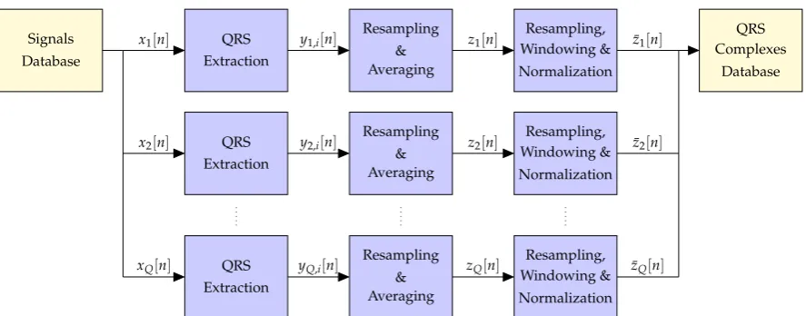
The block diagram of the pre-processing stage is shown in Figure2.5Firstly, all the QRS complexes are extracted separately from each of theQavailable ECGs, and those patients for which a significant number of QRS complexes cannot be reliably obtained are removed from subsequent stages. After resampling to the maximum length of all the QRS complexes found for each of the remainingQ0 ≤Q patients, an individual average QRS complex is obtained per patient. Then, a second resampling stage is applied to the average QRS complexes of all theQ0valid patients to ensure that they have the same length, followed by a windowing stage to obtain initial and final samples equal to zero, and a normalization to remove the mean and enforce unit energy on all the signals. Finally, theseQ0 waveforms are stored in a QRS complexes database and used to construct the desired overcomplete dictionary. In the sequel, we provide a detailed description of each of the blocks in Figure2.
3.2.1. QRS Extraction
The first pre-processing step consists in extracting all the QRS complexes from each of theQ ECGs,xq[n]forq=1, . . . ,Q. In order to attain this goal, we follow the approach described in [27]:
1. Apply a 4th order Butterworth bandpass filter with cut-off frequencies fc1=1 Hz and fc2=40 Hz to remove noise and interferences. Forward-backward filtering, with an appropriate choice of the initial state to remove transients [28], is used to avoid phase distortion.
2. Locate the positions of the R waveforms using the well-known Pan-Tompkins QRS detector [29].
4 https://www.physionet.org/physiobank/database/ptbdb/
5 Let us remark that we focus here on the QRS complexes because they are the most relevant waveforms that can be found in
Signals Database
x1[n] QRS
Extraction
y1,i[n]
Resampling & Averaging
z1[n]
Resampling, Windowing & Normalization
x2[n] QRS
Extraction
y2,i[n]
Resampling & Averaging
z2[n]
Resampling, Windowing & Normalization
xQ[n] QRS
Extraction
yQ,i[n]
Resampling & Averaging
zQ[n]
Resampling, Windowing & Normalization
¯ z1[n]
¯ z2[n]
¯ zQ[n]
QRS Complexes
Database
Figure 2.Block diagram of the pre-processing stage applied before the creation of the dictionary.
3. Determine the fiducial points that mark the beginning and end of the QRS complexes by tracking backwards and forward from the R peaks, estimating the QRS onset and offset points using the minimumradius of curvaturetechnique, as described in Section 4.2 of [27].
This approach results inQ0 =44 valid subjects (i.e.,≈84, 6 % out of theQ=51 available individuals), for which a significant and variable number of QRS complexes (yq,i[n]for 1≤q≤Q0, 1≤i≤Pqand 0≤n≤ Lq,i−1), with a variable length of samples for each of them, are extracted for the database used. A total of 6266 QRS complexes are extracted, implying an average of 142,4 QRS complexes per patient (with a maximum of 194 QRS complexes obtained from a single subject) with lengths from 90 to 124 samples (i.e., from 90 to 124 ms).
3.2.2. Resampling and Averaging
In order to compute an average QRS complex for each individual, we need to work with QRS complexes that have a fixed length. The easiest solution to achieve this goal is resampling the extracted QRS complexes to the maximum length for each patient,Lqmax=max1≤i≤PqLq,i≤ Lmax= max1≤q≤Q0Lqmax = 124 samples. A change in the sampling rate of discrete time signals can be
accomplished by means of interpolation and decimation [30]. If thei-th QRS complex (i=1, . . . ,Pq) has a length Lq,i ≤ Lqmax samples and Mq,i = GCD(Lq,i,Lqmax), with GCD denoting the greatest common divisor, then we need first to interpolate by a factorLqmax/Mq,iand then to decimate by a factorLq,i/Mq,i(i.e., the fractional resampling rate isLqmax/Lq,i≥1).
The aforementioned approach includes a digital lowpass antialiasing filter between the interpolator and the decimator, with a cut-off frequencyωqc,i = πMq,i/L
q
1. From thei-th QRS complex signal,yq,i[n]forn=0, 1, . . . ,Lq,i−1, we first construct the following two sequences:
y(`q,i)[n] =yq,i[n]−yq,i[0], y(rq,i)[n] =yq,i[n]−yq,i[Lq,i−1],
which are not likely to be affected by the edge effect on their leftmost and rightmost samples respectively.
2. We perform the resampling by the factorLq,i/Limaxseparately ony (q,i)
` [n]andy
(q,i)
r [n], obtaining
two resampled sequences ˜y(`q,i)[n]and ˜y(rq,i)[n]. 3. The desired resampled sequence is finally given by
˜ yq,i[n] =
˜
y(`q,i)[n], 0≤n≤jN2 Lqmax Lq,i
k
−1; ˜
y(rq,i)[n],
j
N 2
Lqmax Lq,i
k
−1<n≤jNLqmax Lq,i
k
−1. (6)
Figure3shows the leftmost and rightmost samples corresponding to one of the resampled QRS complexes (from patient 214 in the PTB database) when resampling is performed directly onyq,i[n]. The edge effect on the left and right parts of the signals (i.e., the deviation of the red line w.r.t. the desired values indicated by the black dots) is evident in this case. On the other hand, when the proposed approach is applied, the resampled sequence ( ˜yq,i[n]) is not affected by the edge effect neither on its left side nor on its right side, as seen in Figure3.
Figure 3.Leftmost and rightmost samples of an original QRS complex (from patient 214 in the PTB database) and its resampled version with and without edge effects.
Finally, the averaged QRS complex for each patient is obtained simply by computing the sample mean for each time instant:
zq[n] = 1 Pq
Pq
∑
i=1 ˜
yq,i[n], (7)
withPqdenoting the number of QRS complexes found in theq-th ECG. 3.2.3. Windowing and Normalization
After averaging, all the averaged QRS complexes are resampled again in order to obtainQ0signals with the same number of samples,Lmax=Lmaxq forq=1, . . . ,Q0, using a resampling factorLmax/Lqmax. Then, the resulting signals are windowed to ensure a smooth decay of the QRS complexes towards zero, and normalized by removing their mean and dividing by their standard deviation. The signals that are finally stored in the QRS complex database are
¯
zq[n] =w[n]× ˜
zq[n]−µq
where ˜zq[n]are the averaged QRS complexes after the second resampling stage (i.e., after ensuring that their sample length is equal toLmax),µqandσqare their sample mean and standard deviations, respectively,
µq= 1
Lmax Lmax−1
∑
n=0
zq[n], (9)
σq=
v u u
t 1
Lmax−1 Lmax−1
∑
n=0
(zq[n]−µq)2, (10)
andw[n] is the window used in this case, a window that follows the spectral shape of the raised cosine filter, widely used in digital communications [31], in the time domain: w[n] = wc(nTs)for n=−(Lmax−1)/2, . . . ,−1, 0, 1, . . . ,(Lmax−1)/2, with
wc(t) =
1, |t| ≤(1−α)T0;
1 2
h
1+cos π
2αT0|t−(1−α)T0|
i
, (1−α)T0<|t|<(1+α)T0, (11)
T0 = Lmax−1
1+α Ts
2, andαdenoting the roll-off factor that controls the decay ofwc(t)towards zero: for
α=0 we have a rectangular window that abruptly goes to zero at±T0, whereas forα=1 the window
is bell-shaped and starts decaying smoothly towards zero immediately after|t| >0. This window, whose time-domain shape is shown in Figure4for several values ofα, ensures that the central samples
of the QRS complexes remain undistorted, while their amplitudes decay slowly towards zero at the borders. Throughout the paper, we usedα=0.25.
Figure 4.Several examples of the raised cosine window used forTs=1 ms,Lmax=201, and different values of the parameterα.
3.3. Dictionary Construction
After the pre-processing described in the previous section, we haveQ0 ≤ Qwaveforms from different patients stored in the QRS complexes database. These waveforms ( ¯zq[n]for 1≤q≤Q0and 0≤ n ≤ Lmax−1) could be directly used to build the sub-dictionaries. However, they are highly correlated and thus the resulting dictionary would provide a poor performance and lead to a high computation time. Therefore, in order to obtain a reduced dictionary composed of distinct shapes, we perform the procedure described in the following sections.
3.3.1. Selection of the First Atom
1. Compute Pearson’s correlation coefficient among each pair of waveforms in the QRS complexes database,6
ρij= Cij
q
CiiCjj
=Cij, (12)
whereCijdenotes the cross-covariance between thei-th andj-th waveforms at lag 0 (i.e., without any time shift), and the last expression (ρij=Cij) is due to the energy normalization described in Section3.2.3, which implies thatCii=0∀i.
2. Select the waveform with the highest average correlation (in absolute value) with respect to all the other candidate waveforms, i.e.,
`0=arg maxi=1,...,Q0
Q0
∑
j=1
|ρij|, (13)
which corresponds to the most representative waveform of all the candidate waveforms.
3.3.2. Selection of Additional Atoms
If desired, additional atoms can be selected. These atoms should be constructed using highly correlated waveforms with respect to the remaining candidates (to obtain representative dictionary atoms), as well as with low absolute correlation with respect to already selected waveforms (to avoid similar atoms). Here, we propose to use the following procedure to select a total ofKrepresentative waveforms:
1. Set the number of accepted atoms equal to one (r = 1), the pool of candidate waveforms as
C = {1, . . . ,`0−1,`0+1, . . . ,Q0}(i.e., all the waveforms except for the one selected for the first atom), the pool of accepted waveforms asA ={`0}, and construct a reduced correlation matrix by removing the row and column corresponding to the first atom selected from the global correlation matrixC:
Cr =
"
C1:`0−1,1:`0−1 C1:`0−1,`0+1:Q0 C`0+1:Q0,1:`0−1 C`0+1:Q0,`0+1:Q0
#
. (14)
2. WHILEk<K:
(a) Select, from the remaining waveforms in the pool of candidates, the one with the highest average correlation (in absolute value) with respect to all the other candidate waveforms in the pool, i.e.,
`k=arg maxi=1,...,Q0−k
Q0−k
∑
j=1
|Cr(i,j)|. (15) (b) Compute the maximum correlation (in absolute value) between the selected candidate and
all the already accepted atoms,
ρmax= max
i=0,...,k−1|Cr(`k,`i)|. (16) (c) Remove the`k-th waveform from the pool of candidates (i.e., setC=C \ {`k}), and construct
a new reduced matrix (Cr) by removing the`k-th row and column from the currentCr. (d) IFρmax < γ(with 0 ≤ γ ≤ 1 denoting a pre-defined threshold),THEN add the selected
waveform to the pool of accepted atoms (i.e.,A=A ∪ {`k}), and setk=k+1. END
6 In practice, this only has to be doneQ0(Q0−1)/2 times, since
t (ms)
0
20
40
60
80
100
120
A (mV)
-3
-2
-1
0
1
2
3
Figure 5.Q0=44 reliable average QRS complexes extracted from theQ=51 healthy patients in the PTB database [26] after resampling, windowing and normalization.
3.3.3. Construction of the Multi-Scale Dictionary
Finally, theKselected waveforms are resampled in order to obtain a multi-scale sub-dictionary composed ofRdifferent time scales. Note that the total number of waveforms is thusP=KR. In this case, we have usedR= 11 different time scales spanning the typical durations of QRS complexes: 60, 70, . . . , 160 ms. Note also that the global dictionary is simply obtained by performingN−M different time shifts of the resulting sub-dictionary [13].
4. Numerical Results
In this section, we first detail the construction of the dictionary and then we apply the resulting dictionary to perform the sparse reconstruction of the signals from different patients.
4.1. Dictionary Construction
i
0
10
20
30
40
j
0
10
20
30
40
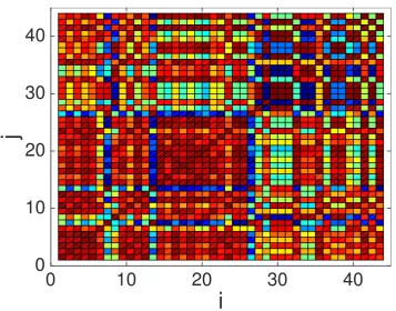
Figure 6. Color map showing the absolute value of the correlation coefficient,|ρij|, for theQ0 =44
average QRS waveforms. Dark red colors indicate values close to 1, whereas dark blue colors indicate values closer to 0.
Figure 7.K=6 atoms selected from theQ0=44 reliable average QRS complexes obtained from the Q=51 healthy patients in the PTB database, using a thresholdγ=0.9.
order to construct the multi-scale and over-complete dictionary. However, in Figure6we also notice that some waveforms exhibit low correlation values (as shown by blue points). This motivates us to explore here the performance as more than one atom is extracted from the pool of average QRS complexes shown in Figure5in order to construct the dictionary.
In order to build dictionaries composed of different waveforms, we have tested several threshold levels: γ = 0.1, 0.2, . . . , 0.9. Note that the largest the value ofγthe less restrictive the condition to
incorporate a new atom to the dictionary, and thus the largest the number of final atoms (K) used: forγ=0 we would always obtainK =1 atoms (since no new atoms can be incorporated after the
first one), whereas forγ=1 we would obtainK=Q0(as all waveforms would be considered valid).
Following this approach, we obtainK=1 atoms forγ≤0.2,K=2 atoms for 0.3≤γ ≤0.6,K =3
atoms whenγ=0.7,K=4 atoms whenγ=0.8, andK=6 atoms whenγ=0.9. Figure7shows the
six atoms selected forγ=0.9. Note that, since we follow a deterministic procedure, the first atom is
the one obtained forK=1 (i.e., whenγ≤0.2), the first and second ones are those obtained forK=2
(i.e., for 0.3≤γ≤0.6), and so on.
selected waveforms), the size of the matrix dictionary ranges fromN×11(N−M) =115200×1265440 forK=1 up toN×66(N−M) =115200×7592640 forK=6.
Figure 8.Multi-scale dictionary constructed using theK=6 most representative waveforms shown in Figure7.
4.2. Sparse ECG Representation
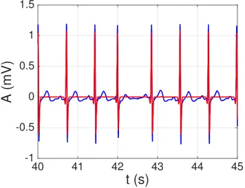
Now we test the constructed dictionary on 21 recordings corresponding to 17 healthy patients from the PTB database. Our main goal in this section is determining whether the constructed dictionary (which is not patient-specific) can be effectively used to perform a sparse representation of ECG signals from multiple patients. In order to solve (5), we use the CoSA (Convolutional Sparse Approximation) algorithm recently proposed in [21], which allows us to process theN≈115200 samples (almost 2 minutes of recorded time) of the whole signal at once (i.e., without having to partition it into several segments that have to be processed separately) in a reasonable amount of time. Since several signals showed a significant degree of baseline wander, before applying CoSA all signals were filtered using a third-order high-pass IIR (infinite impuse response) Butterworth filter designed using Matlab’s filterDesigner tool: stop-band frequency fstop = 0.1 Hz, pass-band frequency fpass = 1 Hz, minimum stop-band attenuation Astop = 40 dB, and maximun pass-band attenuation Apass = 1 dB. Forward-backward filtering was applied again to avoid phase distortion. An example of the reconstructed signal usingK=1 andλ=20 is shown in Figure9. Note that all the QRS complexes
(our main goal here) are properly represented by the sparse model. By increasing the number of signals (K), and especially by decreasing the sparsity factor (λ), a better model that also includes the P
and T waveforms can be obtained. However, let us remark that this is not our main goal. Indeed, a better option to model the P and T waveforms would be constructing specific dictionaries of P and T waveforms: either using synthetic waveforms (e.g., Gaussians) or applying the proposed approach to construct real-world dictionaries of P and T waveforms. We intend to explore this issue in future works.
In order to measure the effectiveness of the proposed approach, we use several performance metrics that measure both the model’s sparsity and its accuracy in representing the original signal. On the one hand, the sparsity is gauged by the coefficient sparsity (C-Sp),
C-Sp (%)= kβk0
(N−M)P×100 (17)
which measures how many coefficients (out of the total ones) are required to represent the signal, and the signal sparsity (S-Sp),
S-Sp (%)= kxk0
N ×100 (18)
which measures how many samples of the signal’s approximation (out of the total number of samples) are equal to zero. Note thatk · k0indicates theL0“norm” of a vector, i.e., its number of non-null elements. On the other hand, the reconstruction error is measured by the normalized mean squared error (NMSE) and its logarithmic counterpart, the reconstruction signal to noise ratio (R-SNR):
NMSE (%)= kx−Aβk 2 2
kxk2 2
×100 (19)
R-SNR (dB)=10·log10(NMSE), (20)
wherek · k2denotes theL2norm of a vector.
The results, for the four performance measured previously described, are displayed in Figure
t (s)
40
41
42
43
44
45
A (mV)
-1
-0.5
0
0.5
1
1.5
Figure 9.Example of sparse ECG representation with the derived dictionary for a segment of signal 121 from the PTB database. Real signal in blue; sparse representation (QRS complexes) in red.
patients in the training set: patients 104, 105, 117, 121, 122, 131, 150, 155, 156, and 169. On the right hand side, we show the results (mean value and standard deviation again) for the 11 signals in the test set: patients 116, 166, 172, 173, 233 (5 recordings), 255, and 266. Note the large sparsity attained in all cases (especially asλincreases), and the good reconstruction error for small/moderate values ofλ
(i.e.,λ≤5). Note also the improvement in performance when incorporating additional waveforms to
the dictionary (e.g., forλ=2 there is a 3.32 dB improvement in mean R-SNR for the patients in the
test set when usingK=6 instead ofK=1), although this comes at the expense of a reduction in the signal sparsity (e.g., for the same case, the mean S-Sp goes down by 4.2% when usingK=6 instead of K=1).
Finally, we applied the Pan-Tompkins algorithm to the reconstructed signal in order to test whether the sparse model introduced some distortion in the location of the QRS complexes. As a result, we found that all the QRS complexes were always properly detected and located within 2 samples (i.e.,±2 ms) of the QRS complexes found in the original signal, even in the sparsest case (i.e., with K=1 andλ=20). Therefore, if we are only interested in the QRS complexes or some analysis derived
from them (e.g., heart rate variability studies), the proposed model is a very good option to construct a sparse model that keeps all the relevant information.
Figure 10.Different performance metrics. Left hand side: results on signals from training set. Right hand side: results on signals from test set.
4.3. Sparse ECG Representation of Other Channels
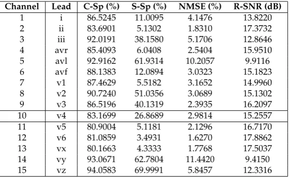
Finally, in this section we investigate the feasibility of using the dictionary learnt on lead V4 to represent ECGs recorded in other leads. In order to do so, we use the constructed dictionary to model all the 15 channels available for patient 104. Table1displays the results forλ=1 andK=2, showing
leads (ii, avr, v5, v6 and vx) in terms R-SNR is better than for lead v4, which was used to construct the dictionary, and poor R-SNR results were only attained for leads avl and vy. Similar conclusions were obtained when considering other values ofλandK. Overall, this shows the feasibility of constructing a
single multi-scale and overcomplete dictionary (possibly using QRS complexes extracted from several leads) for multiple channels.
Table 1.Performance of the constructed dictionary (using waveforms extracted from lead v4) on other leads from patient 104.
Channel Lead C-Sp (%) S-Sp (%) NMSE (%) R-SNR (dB) 1 i 86.5245 11.0095 4.1476 13.8220 2 ii 83.6901 5.1302 1.8310 17.3732 3 iii 92.0191 38.1580 5.1706 12.8646 4 avr 85.4093 6.0408 2.5404 15.9510 5 avl 92.9162 61.9314 10.2057 9.9116 6 avf 88.1383 12.0894 3.0323 15.1823 7 v1 87.4629 5.5182 3.1652 14.9960 8 v2 90.7240 51.0356 3.0689 15.1302 9 v3 86.5196 40.1319 2.3935 16.2097 10 v4 83.1699 26.8689 2.9814 15.2557 11 v5 80.9004 5.1181 2.1296 16.7170 12 v6 81.0859 3.4931 1.6270 17.8862 13 vx 80.1663 4.3333 1.7768 17.5037 14 vy 93.0671 62.7804 11.4420 9.4150 15 vz 94.0583 69.9991 5.8457 12.3316
5. Conclusions
In this paper, we have described a novel mechanism to derive a realistic, multi-scale and overcomplete dictionary from recorded real-world ECG signals. The dictionary is constructed offline, thus avoiding the computational burden of on-line approaches and ensuring the scalability of the proposed methodology for large data sets with many individuals and/or sample sizes. The obtained dictionary has then been used to obtain an accurate sparse representation of several ECGs recorded from healthy patients, showing that it is able to properly capture all the QRS complexes without introducing false alarms. Future lines include testing the proposed approach on a larger number of patients (especially including subjects with cardiac pathologies), the construction of dictionaries composed of multiple waveforms (e.g., P and T waveforms), and the combination of waveforms extracted from real patients with synthetic waveforms.
Author Contributions: Conceptualization, D.L.; methodology, D.L. and D.M.; software, D.L., D.M. and T.T.; validation, D.L.; data curation, D.M.; original draft preparation, D.L.; review and editing, D.M. and T.T.
This research was funded by Ministerio de Economía y Competitividad (Spain) through the MIMOD-PLC project (grant number TEC2015-64835-C3-3-R).
Conflicts of Interest:The authors declare no conflict of interest. The funders had no role in the design of the study; in the collection, analyses, or interpretation of data; in the writing of the manuscript, or in the decision to publish the results.
Bibliography
1. Sörnmo, L.; Laguna, P.Bioelectrical signal processing in cardiac and neurological applications; Academic Press, 2005.
3. Tibshirani, R. Regression shrinkage and selection via the Lasso. Journal of the Royal Statistical Society. Series B (Methodological)1996, pp. 267–288.
4. Elad, M.Sparse and Redundant Representations: From Theory to Applications in Signal and Image Processing; Springer, 2010.
5. Kreutz-Delgado, K.; Murray, J.F.; Rao, B.D.; Engan, K.; Lee, T.W.; Sejnowski, T.J. Dictionary learning algorithms for sparse representation.Neural computation2003,15, 349–396.
6. Rubinstein, R.; Bruckstein, A.M.; Elad, M. Dictionaries for sparse representation modeling. Proceedings of the IEEE2010,98, 1045–1057.
7. Tosic, I.; Frossard, P. Dictionary learning. IEEE Signal Processing Magazine2011,28, 27–38.
8. Billah, M.; Mahmud, T.; Snigdha, F.; Arafat, M. A novel method to model ECG beats using Gaussian functions. Proc. 4th IEEE Int. Conf. on Biomedical Engineering and Informatics (BMEI), 2011, Vol. 2, pp. 612–616.
9. Monzón, S.; Trigano, T.; Luengo, D.; Artés-Rodríguez, A. Sparse spectral analysis of atrial fibrillation electrograms. Proc. IEEE Int. Workshop on Machine Learning for Signal Processing (MLSP). IEEE, 2012, pp. 1–6.
10. Trigano, T.; Kolesnikov, V.; Luengo, D.; Artés-Rodríguez, A. Grouped sparsity algorithm for multichannel intracardiac ECG synchronization. Proc. 22nd European Signal Processing Conference (EUSIPCO), 2014, pp. 1537–1541.
11. Divorra-Escoda, O.; Granai, L.; Lemay, M.; Hernandez, J.M.; Vandergheynst, P.; Vesin, J.M. Ventricular and atrial activity estimation through sparse ECG signal decompositions. Proc. of the IEEE Int. Conf. on Acoustics, Speech and Signal Processing (ICASSP), 2006, Vol. II, pp. 1060–1063.
12. Fira, M.; Goras, L.; Barabasa, C.; Cleju, N. On ECG compressed sensing using specific overcomplete dictionaries. Advances in Electrical and Computer Engineering2010,10, 23–28.
13. Luengo, D.; Monzón, S.; Trigano, T.; Vía, J.; Artés-Rodríguez, A. Blind analysis of atrial fibrillation electrograms: a sparsity-aware formulation. Integrated Computer-Aided Engineering2015,22, 71–85. 14. Luengo, D.; Vía, J.; Monzón, S.; Trigano, T.; Artés-Rodríguez, A. Cross-products LASSO. Proc. IEEE Int.
Conf. on Acoustics, Speech and Signal Processing (ICASSP), 2013, pp. 6118–6122.
15. Wang, C.; Liu, J.; Sun, J. Compression algorithm for electrocardiograms based on sparse decomposition. Frontiers of Electrical and Electronic Engineering in China2009,4, 10–14.
16. Mailhé, B.; Gribonval, R.; Bimbot, F.; Lemay, M.; Vandergheynst, P.; Vesin, J.M. Dictionary learning for the sparse modelling of atrial fibrillation in ECG signals. Proc. of the IEEE Int. Conf. on Acoustics, Speech and Signal Processing (ICASSP), 2009, pp. 465–468.
17. Polania, L.F.; Barner, K.E. Multi-scale dictionary learning for compressive sensing ECG. IEEE Digital Signal Processing and Signal Processing Education Meeting (DSP/SPE), 2013, pp. 36–41.
18. Fira, M.; Goras, L.; Barabasa, C.; Cleju, N. ECG compressed sensing based on classification in compressed space and specified dictionaries. Proc. of the 19th European Signal Processing Conference (EUSIPCO), 2011, pp. 1573–1577.
19. Fira, M.; Goras, L.; Barabasa, C. Reconstruction of compressed sensed ECG signals using patient specific dictionaries. Proc. Int. Symp. on Signals, Circuits and Systems (ISSCS), 2013, pp. 1–4.
20. Fira, M.; Goras, L. On projection matrices and dictionaries in ECG compressive sensing — A comparative study. 12th Symposium on Neural Network Applications in Electrical Engineering (NEUREL), 2014, pp. 3–8.
21. Trigano, T.; Shevtsov, I.; Luengo, D. CoSA: An accelerated ISTA algorithm for dictionaries based on translated waveforms. Signal Processing2017,139, 131–135.
22. Luengo, D.; Meltzer, D.; Trigano, T. Sparse ECG Representation with a Multi-Scale Dictionary Derived from Real-World Signals. Proc. of the 41st International Conference on Telecommunications and Signal Processing (TSP), 2018, pp. 1–5.
23. McSharry, P.E.; Clifford, G.D.; Tarassenko, L.; Smith, L.A. A dynamical model for generating synthetic electrocardiogram signals. IEEE transactions on biomedical engineering2003,50, 289–294.
24. Goldberger, A.; others. Physiobank, physiotoolkit, and physionet. Circulation2000,101, e215–e220. 25. Hu, X.; Liu, J.; Wang, J.; Xiao, Z. Detection of onset and offset of QRS complex based a modified triangle
26. Bousseljot, R.; Kreiseler, D.; Schnabel, A. Nutzung der EKG-Signaldatenbank CARDIODAT der PTB über das Internet.Biomedizinische Technik/Biomedical Engineering1995,40, 317–318.
27. Israel, S.; others. ECG to identify individuals. Pattern Recognition2005,38, 133–142.
28. Gustafsson, F. Determining the initial states in forward-backward filtering. IEEE Transactions on Signal Processing1996,44, 988–992.
29. Pan, J.; Tompkins, W.J. A real-time QRS detection algorithm.IEEE Transactions on Biomedical Engineering 1985,32, 230–236.
![Figure 5. Q′ = 44 reliable average QRS complexes extracted from the Q = 51 healthy patients in thePTB database [26] after resampling, windowing and normalization.](https://thumb-us.123doks.com/thumbv2/123dok_us/1005214.1600378/10.595.121.476.89.365/reliable-complexes-extracted-patients-database-resampling-windowing-normalization.webp)