© 2015 IJSRST | Volume 1 | Issue 5 | Print ISSN: 2395-6011 | Online ISSN: 2395-602X Themed Section: Science and Technology
An Approach to Survival Analysis when Frailty is Evident
Jude Nwoji Oguejiofor
1, AbubakarBoyi Dalatu
2, KabiruYanusa Gorin Dikko
2 1Department of Computer Science, Waziri Umaru Federal Polytechnic Birnin Kebbi, Nigeria 2
Department of Statistics, Waziri Umaru Federal Polytechnic Birnin Kebbi, Nigeria
ABSTRACT
The problem with survival estimation using traditional life-table method alone is not only grouping of survival times, but also its insensitivity to existence of frailty in population. In this work, an approach has been proposed for the analysis of time from infection to occurrence of an event vis-à-vis the contributions of frailty along with some covariates. The approach involves the use of nonparametric product limit otherwise known as the Kaplan-Meier (KM) to estimate individual survivals and the use of frailty estimation method to estimate the hazard. In a simulation, the life-table and product limit methods were compared using the standard error estimates and plots of the empirical survivor function. While empirical estimates did not show significant differences, the product limit plot is more informative than the life table plots. The result of hazard estimation shows that event is largely caused by the baseline hazard with significant contribution from frailty and little contribution from age. There is also significant association between individual’s events possibly as a result of frailty. This procedure will find wider application in survival estimation in a population-based setting.
Keywords : Survival Estimation, Empirical Survivor Function Plot, Frailty
I.
INTRODUCTION
Survival data are summarized through the estimate of survival function and hazard function. Several non-parametric methods which do not require any specific assumption about the underlying distribution of survival time have been discussed by several authors during the past six decades or so Ramadurai et al( 2011). Many researchers have written reports about life table. Berkson et al(1950), Gehan, (1969). Petoet al (1976) has published an outstanding review of statistical methods related to clinical trials. The development of the field that have had the most thoughtful impact on clinical trials are the Kaplan-Meier (Product limit) (1958) method for estimating the survival function. A method developed by Mantel (1966) was used to compare two survival patterns in the life table analysis. This method was used by Myers (1969) to analyze the survival experience for male patients with localized cancer of rectum diagnosed in Connecticut from 1935 – 1944 and 1945 – 1954.
2.0 Existing Work
2.1 The Empirical Survivor Function
The survivor function ( )S t , is the probability that an individual survives for a time greater than or equal to t. The function can be estimated
Number of Individuals with survival times t ˆNumber of Individuals in the data set
S t
(2.1)
or
S t
ˆ
( ) 1
F t
ˆ
( )
, where ˆF (t) is the empirical cumulative distribution function, that is, the ratio of the total number of individuals alive at time t to the total number of individuals in the study. The estimatedsurvivor function
S t
ˆ( )
is assumed to be a constant2.2 Life-Table estimate of the survivor function
The life-table estimate of the survivor function is obtained by first dividing the period of observation into series of time intervals. Suppose that in the jth interval,
the probability of death is estimated by dj/ '
j
n
, so that thecorresponding survival probability is
(
n
'j
d
j) /
n
'j.
nowconsider the probability that an individual survives
beyond time
t k
k',
1, 2,..., ,
m
that is, until sometime after the start of the kth interval. This will be the product of the probabilities that an individual survives beyond the start of the kth interval and through each of the k – 1 preceding intervals, and so the life-table estimate of the survivor function is given by' ' 1 *( ) ( ) k j j j j n d S t n
(2.2)' '
1
,
1, 2,..., .
k k
t
t t
k
m
On the assumption that censoring occur uniformly over the intervals. A graphical estimate of the survivor function will then be a step-function with constant values of the function in each time interval. However, life table method requires grouping of survival times which may lead to loss of information and possible biasness. The method only finds the estimates of the survivor function. It does not address such important aspects as randomness and covariate effects.
2.3 Kaplan Meier (product-limit) estimate of the survivor function
To obtain the Kaplan- Meier estimate, a series of time intervals is constructed, as for the life-table estimate. However, each of these intervals is designed to be such that one death time is contained in the interval, and this death time is taken to occur at the start of the interval. We now make the assumption that the deaths of the individuals in the sample occur independently of one another. Then, the estimated survivor function at any time, t, in the kth constructed time interval from t(k) to
t(k+1) , k = 1, 2, …., r, where t(j+1)is defined to be ∞, will
be the estimated probability of surviving beyond t(k).
This is actually the probability of surviving through the
interval from
t
( )k to( )k (k 1),
1, 2,...., ,
ˆ
( ) 1
(1)t
t
t
k
r with S t
for t
t
and all preceding intervals, and leads to the Kaplan-Meier estimate of the survivor function, which is given by
*
1
ˆ
k j jj j
n
d
S t
n
(2.3)For
t
( )k
t
t
(k1),k
1, 2,...., ,
r with S t
ˆ
( ) 1
for t
t
(1), and where t(r+1) is taken to be ∞. However, this method alone cannot be used to estimate patients survival alongside the influence of covariates and frailty at a particular event time t.The standard error for the Kaplan-Meier estimate is given by
1 2 1ˆ ˆ k j
j j j j
d Se S t S t
n n d
for
t
k
t
t
k1(2.4) While the standard error (se) of the life table estimate is given by
1 2 * 1ˆ k i
j j j j
d Se S t S t
n n d
, Collet (2003)
(2.5)
II.
METHODS AND MATERIAL
3.0 Methodology
3.1 Simulation study
The simulation now gives a survival data set from a population with exponentially distributed baseline hazard (due to the distribution of the survival times) and gamma distributed frailty condition.
Below is a sample from the 500 generated survival data.
Each observation corresponds to α, the variable id being the patient’s code. The time (in days) from infection of an event or censoring is stored in time, while status is 1 when event has occurred and 0 for censored observations. Two other covariates may contribute: age, the age of the patient in years, and sex, being 1 for males and 2 for females. The variable frail is the frailty value for each individual which is assumed to have a gamma distribution.
The hazard of event (presented in frailty model form) will be modeled as a function of the patient’s age and sex. An R package parfm function is used to do the analysis.
3.2.0 Estimation of Frailty
Estimates of , , are obtained by maximizing the
marginal log-likelihood; this can be easily done if one is
able to compute higher order derivatives
L
q
of theLaplace transformed up to
q
max
d
1,...,
d
s
3.2.1 Gamma Frailty
A gamma frailty term is a random variable
*
~ Gam
z
with probability density function
1 1 1 exp / , 0, 1 z u f z
(3.1)where
is the gamma function. It corresponds to aGamma distribution Gam
,
with
fixed to 1 asstated earlier Collet (2003), Rotolo et al (2012) for identifiability. Its variance is then
. The associated Laplace transform is given by
11
,
0,
L s
s
s
(3.2)and it is easy to show that, for q1,
1
0
1 1 1 .
q
q q
q
l
L s
s l
L s
(3.3)Therefore, in equation (1.5), we have (i.e. the
log-likelihood)
1
0
1
log
1
log 1
log 1
q
q q
l
L
s
q
s
l
, Rotolo et al (2012) (3.4)
For the Gamma distribution, the Kendall’s Tau Hougaar et al (2000), which measures the association between any two event times from the same cluster in the multivariate case, can be computed as
0,1 2
(3.5)
III.
RESULT AND DISCUSSION
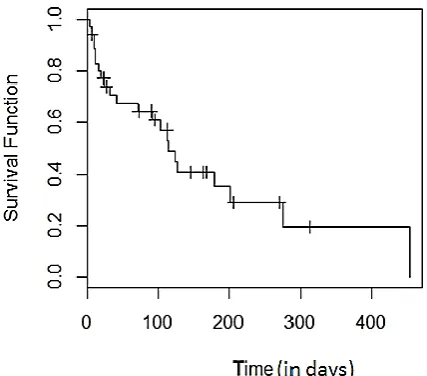
4.1 Plots of the Empirical Survivor Function Using the Product-Unit (K-M) Method
Fig. 4.2: KM Plot of Empirical Survivor Function, when sample size n = 100
Fig. 4.3: KM Plot of Empirical Survivor Function, when sample
size n = 285
Fig. 4.4: KM Plot of Empirical Survivor Function, when sample size n = 500
4.2 Plots of the Empirical Survivor Function Using the Life-table Method
Fig 4.2a. plot of the survivor function; sample size n=50
Fig 4.2b ; plot of the survivor function; Sample size n=500; interval length is 29
Fig 4.2c. plot of the survivor function, sample size n=500 ; interval length is 50
(in days)
(In days)
Fig 4.2d. plot of the survivor function, sample size n=500 ; interval length is 100
4.3 Discussion
When the sample size is at n50,n100the empirical
survivor function (esf) plot using K-M method displays good fit(fig 4.1, 4.2, 4.3, and 4.4). It shows decreasing step function behavior with survival function value (1) one at zero (0) survival time. As the survival time increases, the survivor function decreases with constant values between two adjacent death times. The plot of the function display similar behavior and pattern even with large samples as in n500and n285. The plot of the function maintained it defined characteristics i.e. decreasing step function.
On the other hand, when sample size is not large such as n=50, the life-table plot displays the decreasing, step function behavior (fig 4.2a ). But when sample size is large as n=500, the life-table plot though displays decreasing behavior, it is less informative about event times, i.e. it does not show the character of being constant between two adjacent event times. Moreover, when sample size is large, if intervals are not long enough, the life-table curve will be less meaningful.
Table 4.1: Comparison of some survival estimates and their standard error (from the results of the simulation ) of life-table vs Kaplan-Meier (product limit)
A comparative look at the results of the survivor estimates table 4.1 using the two methods (from results of the simulation) shows that when the number of patients at risk are 437, 405, 206 and 176, the respective life table survival estimates are 0.950, 0.913, 0.642 and 0.583; while that of K – M are 0.932, 0.910, 0.606 and 0.549 respectively.
The standard error, which is an essential aid for interpretation of precision, for the said values are; 0.009, 0.013, 0.024 and 0.025 for the life table estimation. While the K–M has 0.012, 0.013, 0.025 and 0.026, which does not show much difference between the survival estimates of the methods and so is the case with the standard error estimates.
4.4 Result of the frailty estimation alongside other covariates
Frailty – Gamma
Baseline hazard – Exponential Loglikelihood – 1625.279
The frailty is estimated alongside age and sex. The result (4.4) shows that age could have a significant impact on the hazard of total blindness given the frailty while it is
not affected by sex. The heterogeneity parameter
i.e. the frailty is estimated at 0.005 leading to a Kendall’s tau equal to 0.002, a value which indicates a very close association between two event times (in this case event between two individuals) in the cluster. The conclusiontherefore is that event in this study is largely caused by the baseline hazard and frailty. The frailty has a gamma distribution evidently because the generated data is a mixture of exponentially distributed times with Poisson status or censoring indicators. The baseline hazards has exponential distribution due to the fact that the survival times (observations) are generated exponentially.
IV.
CONCLUSION
The form of the estimated survivor function and the shape of its plot in life table method is sensitive to the choice of intervals. Though the survival estimates and the standard error estimates obtained using the two methods did not show much differences where the numbers at risk are equal, the empirical survival plot using Kaplan-Meier method is more informative, i.e. it tells more about event times and displays the good feature of being constant between two adjacent event times. Also in the simulated population with exponentially distributed baseline hazard and gamma frailty, the event of interest is found to be largely caused by the baseline hazard with significant contribution of frailty and the covariate age. The covariate sex was not found to have any influence on the occurrence of the event.
V.
REFERENCES
[1] Ardino, V., De Angelis, R., Francis, S. and Grande, E. (2007).Methodology for Estimation of Cancer Incidence Survival and Prevalence in Italian Regions. Tumore 93: 337 – 344.
[2] Berkson, J. and Gage, R. P. (1952).Survival Curve for Cancer Patients Following Treatment. Journal of The American Statistical Association, 47: 501 – 515.
[3] Baili, P., Micheli, A., Angelis, R. D., Weir, H. K., Francis, S., Santaguilic, M., Hakulinen, T., Quaresma, M., Coleman, M. P., and the Concord working group (2008). Life Tables for Worldwide Comparison of Relative Survival for Cancer (Concord Study).Tumori, 94: 658 – 668.
[4] Collet D (2003). Modeling Survival Data in Medical Research. Chapman & Hall/CRC
[5] Cox DR (1972). “Regression Models and Lifetables” Journal of the Royal Statistical Society Series B (Methodological) 34(2) 187 – 220.
[6] Dickman, P. W. (2010). An Introduction and Some Recent Development in Statistical Methods for Population-Based Cancer Survival Analysis. Statistical Methods for Population-Based Cancer Survival Analysis. Milan.
[7] Dickman PW, Hakilinen I (2001). Population Based Cancer Survival Analysis. Chapman & Hall.
[8] Duchateau L, Janssen P (2008). The Frailty Model. Springer-Verlag
[9] Duchateau L, Janssen P, Lindsey P, Legrand C, Nguti R, Sylvester R (2002). “The Shared Frailty Model and the Power of Heterogeneity Tests in Multicenter Trials.” Computational Statistics and Data Analysis, 40(3), 603 – 620. doi:10.1016/S0167-9473(02)00057 – 9.
[10] Geham, E. H. (1969). Estimating Survival Functions From the Life Table. Journal of Chronic Diseases, 21: 629 – 694.
[11] Hanagal D (2011). Modelling Survival Data using frailty models. Chapman & Hall/CRC Press. Taylor and Francis Group, LCC.
[12] Hougaard P (1995). “Frailty Models for Survival Data.” Lifetime Data Analysis,1(3), 255 – 273. doi:10.1007/BF00985760.
[13] Hougaard P (2000). Analysis of Multivariate Survival Data. Springer-Verlag.
[14] Kaplan, E. L., Meier, P. (1958). Nonparametric Estimation From Incomplete Observations. J Am. Stat. Association.55: 457 – 81.
[15] Mantel N (1966). Evaluation of Survival Data and Two New Rank Order Statistics Arising in its Consideration. Cancer Chemotherapy Report, 50, 163 – 170.
[16] Peto, R., Pike, M. C., Armitage, P., Breslow, N. E., Cox, D. R., Howard, S. V., Mantel, N., McPherson, K., Peto, J. and Smith, P. G. (1976). Design and Analysis of Randomised Critical Trials Requiring Prolonged Observation of Each Patient. Introduction and Design. British Journal of Cancer. 34: 585 – 612.
[18] Ravichandran, K., AlHandam, N., Al Dyab, A. (2006). Asian Pacific Journal of Cancer Prevention. Vol. 6.
[19] Rotolo F, Munda M (2012). Parfm; Parametric Frailty Models. R package version 0.66, URL http://CRAN.R-project.org/package=parfm
[20] Therneau TM, Grambsch PM (2000). Modeling Survival Data:Extending the Cox Model. Springer-Verlag.
[21] Vaupel JW, Manton KG, Stallard E (1979). “The Impact of Heterogeneity in Individual Frailty on the Dynamics of Mortality.” Demography, 16(3), 439 – 454.
[22] Wang ST, Klein JP, Moeschberger ML (1995). “Semi-parametric Estimation of Covariate Effects Using the Positive Stable Frailty Model.” Applied stochastic models and data analysis, 11(2), 121 – 133.