3160
PPGA: Partial-Partitioned Greedy Algorithm For
Routing In Mobile Sensor Networks
S. Hemalatha, Dr. E. George Dharma Prakash Raj
Abstract: mobile sensor network can defined as a wireless sensor network in which the sensor nodes are mobile. The mobile sensor networks are much more versatile than the static sensor networks. In this paper location-based routing protocol called Partial-partitioned Greedy Algorithm (PPGA), for mobile sensor networks that consist of frequently moving sensors is proposed. The protocol uses the location information of sensors and the base station to assign a cost function to each sensor node, which is close to the Euclidean length of a sensor node’s shortest path to the base station. A packet is forwarded to the base station using greedy forwarding whenever possible. When a packet reaches sensor nodes near local minimums, where greedy forwarding will be impossible after a number of hops, the packet is forwarded following the high-cost to low-cost rule. Extensive simulations are used to compare the performance of PPGA with Greedy Perimeter Stateless Routing (GPSR) and Ad-hoc On-demand Distance Vector protocol (AODV) in mobile sensor networks. Experimental results show that PPGA achieves higher packet delivery ratio, collision rate, lower average delay and lower energy consumption.
Index Terms: cost function, Euclidean length, high-cost to low-cost rule, hops, local minimums, partial partition. —————————— ——————————
1.
INTRODUCTION
Mobile Sensor Networks (MSNs) are progressively rising in different application spaces, from natural checking to astute modern computerization. In MSNs, the vitality effectiveness during directing activities has been an essential metric on the grounds that common sensor nodes have compelled battery control [1]. Not with standing, the mobility that outcomes from system natural impacts (e.g., wind and water) or from portable articles (e.g., human, creature, robot, and vehicles) can corrupt the vitality proficiency of sensors essentially [2]. Likewise, as mobility increments, directing plans are influenced in various ways. In proactive plans, for example, DSDV [3], the quantity of control messages expands drastically to keep up the course before the connection breaks paying little respect to whether information is being transmitted. Then again, in receptive plans, for example, AODV [4], the sensor nodes find the course to the goal just in the event that they are needed. These plans can likewise lessen the control overhead contrasted with proactive methodologies. Be that as it may, increasingly continuous changes of the topology can prompt a disappointment of the disclosure procedure even under a responsive plan.In this manner, an increasingly proficient and powerful directing plan reasonable for MSNs have to be structured. We center around a hybrid approach that depends on mobility data and accept that every sensor has diverse portability data in a blended sensor system comprising of static and mobile nodes albeit all sensors have a similar mobility model. Most half and half methodologies focus on traffic load thinking about the effect of the region. Be that as it may, in exceptionally versatile sensor arranges, the effect of portability could easily compare to the advantages of the region in light of the fact that most undelivered messages are brought about by broken connections because of node mobility, and the message misfortune can prompt various control messages from continuous course upkeep and monotonous course revelation
endeavors. So as to diminish the control overhead, proposed methodology uses a steady way that is built up between less portable elements using portability data. Partial partitioned greedy algorithm routing, as the name implies, is a routing mechanism that looks for the best opportunity to forward a message towards the destination also in the absence of a connected end-to-end route.
2.
LITERATURE
REVIEW
Alexandre and Antˆonio proposed ADHOP, an energy aware routing algorithm that makes routing decision through the ACO. ADHOP uses residual energy as heuristic information to make routing decisions [5]. ADHOP energy consumption is balanced over the network, the network traffic is distributed, thus reducing the possibility of congestion. Gianpaolo and Matteo proposed CCBR results a higher packet delivery with a low cost of routing, which potentially implies a low power consumption [6]. CCBR is analyzed under different conditions, we were also interested in comparing it with other protocols like gossip and uni. Gossip represents the simplest possible approach to manage a mobile network. Gossip is a structure-less protocol in which nodes send packets probabilistic decision: when a node hears a packet for the first time it retransmit it with a probability. Unicast uses routing tables towards the sink. Messages matching the interests of a sink S (considering both its context and content part) are sent, using link-layer unicast transmissions, hop by hop, up reaching S (different sinks are managed separately).
Xiaoxia, Hongqiang and Yuguang proposed robust routing protocol is capable of selecting the best path in a wide zone. RRP ensures to find the route failure in the wide range of sensor network, and establish the route for data transmission [7]. Siming and others proposed greedy algorithm on static and virtual network to enhance the packet delivery ratio, delay on nodes against traffic etc. This paper the sensor node forward the packet to its nearest node until the packet arrives at the destination [8]. Each node can obtain the locations of neighboring node from the global node location table. And nodes can get their neighbor information from the global link table. Le Zou, Mi Lu, Zixiang Xiong proposed (PAGER-M) Greedy forwarding may fail that has no closer neighbor to the base station. When a packet reaches sensor nodes near a concave node, the packet is forwarded to a neighbor following the high-cost-to low-cost rule. In paper Location information of ————————————————
Hemalatha.S Department of Information technology, Bishop Heber College, Tiruchirappalli-620 017,India. PH-00914312770136. E-mail: [email protected]
Dr. E.George Dharma Prakash Raj,School of Computer Science,
Engineering and Application,Bharathidasan University,
Tiruchirappalli – 620 023, India. E-mail:
3161 sensor nodes are updated in routing table the base station to
assign each sensor node a cost, which is close to a sensor’s shortest path from the base station [9]. PAGER-M reduces path redundancy, transmission failures due to node mobility factor. This algorithm prolong the network life time, reduce the node collision and overhead. Shahzad Ali and Sajjad Madani presented a Distributed Efficient Multi hop Clustering (DEMC) protocol for mobile wireless sensor networks [10]. It is an energy efficient, recovery mechanism used to reduce packet loss. DEMC propose less messages exchanges during cluster head selection. It improves high packet delivery ratio and network lifetime. This algorithm is applied in static and mobile networks. Munuswamy, Jothi Muneeswari and others, proposed virtual force-based intelligent clustering for energy-efficient routing in MWSNs has been proposed for effective and energy-efficient cluster-based routing of data packets collected by mobile sensor nodes in a MWSN. The major advantages of this algorithm are its capability in significantly extending the network lifetime and by managing the mobility of MSWN. VFICEER algorithm reduces the number of hops in routing and uses the Euclidian distance with the probability density function of normal distribution to fix the threshold for clustering, which is used to make effective decisions about routing. Spatiotemporal constraints are used in the form of rules for clustering, re clustering, and cluster head election and to perform routing through the cluster heads using intelligent rules. This algorithm utilize attractive and repulsive forces for finding the cluster members. VFICEER protocol [11] use of virtual force, spatial constraints, and temporal constraints to improve communication in MWSN.
3 PARTIAL
PARTITIONED
GREEDY
ALGORITHM
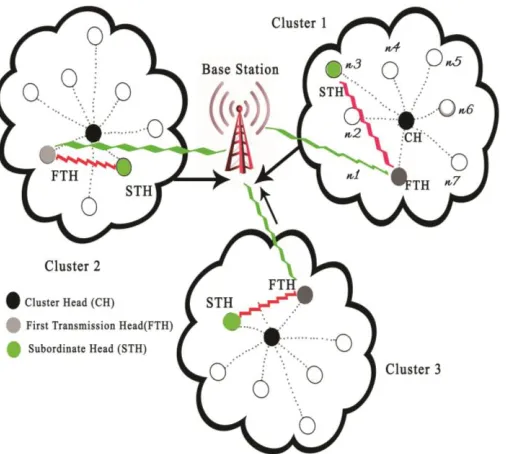
In spite of improving the security and precision of the gathered information, the checking scope of the sensor nodes in the observing region are covered with each other, so the information gathered by the nodes are repetitive . The cluster head selection, the transmission Head selection, choosing the nodes in double CH scenario, the transmission link between CH and TH, the role of TH and the work flow is given in fig 1. All the node in the cluster will be a CH or TH in any occasion but it should be recognized by the prior node with the proper specification. The cluster head will be act as a pioneer node in the cluster and it segregates the work or interlinks the nodes. The transmission head will act like CH but it will be like an agent between the clusters.
Fig1: CH and TH communicating Base station in multiple
clusters
In many cases the TH also acts like CH and in addition with the transmission head. There are few chances for every node to take a lead in the cluster. For that the node has to be scheduled in a proper way. The selection of nodes and the transmission of data’s within the data’s will be discuss clearly in the below case studies. Cluster forming and maintaining the clusters are the two most important categories in cluster scenario. Two circumstances can invoke the cluster upkeep stage, when there is node development outside of its cluster limit and when there is unnecessary battery utilization at the CH. At the point when a common node moves outside of its cluster limit, it is required to locate another cluster head to partner with. In the event that it finds another CH, it hands over to the better and brighter one group. If not, it proclaims itself as a cluster head. Each CH refreshes the measure of expended battery control when it sends and gets packets. On the off chance that the measure of expended battery control turns out to be in excess of a pre-characterized edge esteem then the cluster head leaves and turns into a protocol node. This calculation gives preferred execution over WCA as far as the quantity of reaffiliations, end-to-end throughput, overheads amid the underlying clustering set up stage, and the life expectancy of nodes.
3.1 CLUSTER ISSUES
3162 trades, handling, and vitality. Cluster heads ought to have
higher remaining vitality as contrast with different nodes inside its region.
3.2 CLUSTERHEADSELECTION
During cluster head selection each node calculates weight based on its residual energy and unique node identifier. Cluster Head Selection Algorithm
Start_CH_SelectionAlgorithm() 1. singclusweight=w1×E+w2×I 2. isclusterhead=1
3. maxweight=singclusweight 4. timer=1/singclusweight 5. if (timer<0)
6. CH_Announcment(myID,singclusweight)
ReceiveAnnouncment(SNid,weight) 1. If (isclusterhead==1){
2. If(ownweight<weight){ 3. isclusterhead=0 4. MyCH=SN id 5. maxweight=weight}} 6. else if(isclusterhead==0){ 7. If(maxweight<weight){ 8. MyCH=SN id
9. maxweight=weight}}
Send_Finalized_CH_Announcment() 1. If (isclusterhead==1)
2. Final_CHAnnouncment(myID,singclusweight)
The nodes whose clock terminates first, sends a communicates message 'CH_Announcment (myID,weight)' to its neighbour nodes. After accepting cluster head declaration messages, a node that gets 'CH_Announcment' verifies that whether its own weight is lower when contrasted with weight got from 'CH_Announcment' of neighbouring node or not. In the event that its weight is lower when contrasted with the publicized weight also, on the off chance that the banner 'isclusterhead=1', at that point it will set the banner 'isclusterhead=0' and discount the promoting node as its group head and for the current round it won’t communicate its 'CH_Announcment'.
3.3 ANALYSISOFCHANDTH
In the paper, we assume there are N nodes unevenly distributed in an D X D region, the network region is mentioned as L, k is mentioned as the number of Clusters, A is mentioned as hot area and the number of nodes in the network is mentioned as n . During single frame the energy used in the region of CH is
𝑬𝒏 = 𝑺(𝑬𝒏 + 𝑬 ) ( − 𝟐) + 𝑺(𝑬𝒏 + 𝜺 𝟐
) (2)
Where 𝐸𝑛 the energy is for CH, S is bit message, 𝐸𝑛 is the
energy elected within the region, 𝐷 is the distance between
CH and TH. The Transmission head energy deployed in the single frame is mentioned as
𝑬𝒏 = 𝑺(𝑬𝒏 + 𝑬 ) + 𝑺(𝑬𝒏 + 𝜺 )
𝐷 is the distance between TH and the base station BS. The distance between the non-cluster nodes is mentioned as
𝑬𝒏 = 𝑺(𝑬𝒏 + 𝜺 𝟐
) (4)
Where 𝐷 is the distance between Non cluster node and CH falls within the region.
3.4 MULTIPLE TRANSMISSION HEAD AND SUBORDINATES
The Transmission Head of each cluster receives the signal from the CH and precedes the value to the Base Station. In the absence of CH, Transmission Head (TH) will act as a cluster Head in the region. It will coordinates the other nodes and channelize the communication in the proper way. If the residual energy of the CH is lowered then the CH loses it power and not capable to receive or send the signal among other nodes. Moreover the CH can’t precede the communication to the BS with the minimum residual energy. So automatically the immediate subordinate nodes will do their interlinking process. In the absence of CH, TH may act as a cluster head and it will be called as FTH. FTH is nothing but First Transmission Head that automatically activates the work of CH and channelize the communication properly.
Fig 2: Formation of STH and FTH communication in the
absence of CH
While at the FTH communication to the BS, the Subordinate node of FTH called as STH take position to back up the communication process. This is given in fig 2. The Sub ordinate Transmission Head will do the process of FTH in its absence. It will support the First Transmission Head to do the communication among all the nodes. The Cluster head selects the STH by its high energy next to FTH. In the case of failing FTH residual energy, STH will be in the track to channelize the communication of the cluster. Then STH will get all the previous value of FTH from CH and communicates directly to the BS. The same process will be done simultaneously for all the nodes get diminished.
Possible Ways
3163 CH
TH Or
FTH STH BS
BSCHTH Y Y need No Y
BSCHFTH
STH Y Y N Y
BSFTHSTH N Y Y Y
Fig 3: Signal Indication of nodes
The Signal Indication of all the nodes is given in Fig.3. While in the communication process from the cluster to Base Station, the indication is mentioned in the reverse order. BSCHTH is the first possibility to transmit the signal from cluster to BS. Another possibility of communicating is mentioned as BSCHFTH STH., here the TH will be named as FTH. While FTH residual energy is start diminishing and another subordinate will be selected by the CH named as STH. The third possible way id BSFTHSTH, in the absence of CH automatically FTH and STH will be in the frontline to interlink the nodes communication. At that time FTH will be converted as CH and STH will converted as FTH. This process will be continue until all the nodes will be diminished in the network region.
3.5INTRAANDINTERCLUSTERCOMMUNICATION
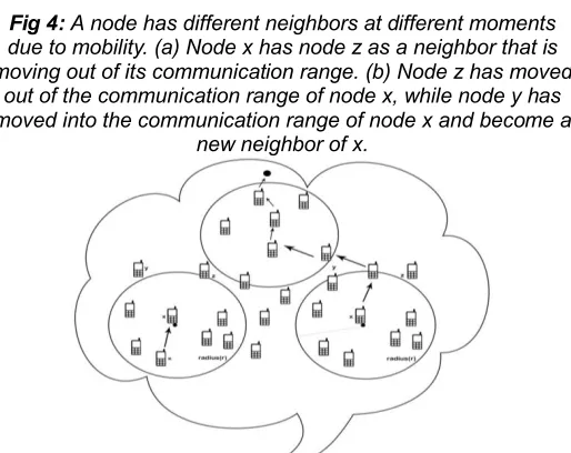
During intra-bunch correspondence, every typical node sends data to its group head (Cluster Head). It is seen during the re-enactments that most of packet loss happens during intra-cluster interchanges when typical nodes attempt to send data to their individual CH and because of node mobility either CH moves from the transmission scope of ordinary node or Vice versa. During this stage, each group head gathers data from its encompassing nodes that are related with that CH and after that sends the total information to the destination. During the Inter Cluster Communication, CH sends the information to neighboring node or the nearest high residual energy node. No two CH will be act in the cluster region. There won’t be a two Cluster heads in the cluster region; instead the above process of CH, TH, FTH, and STH will do the process in the prescribed way. The nodes moving inside and outside of the cluster region will happen normally. The below fig. 4 clearly demonstrates the nodes interlink among the cluster region.
Fig 4: A node has different neighbors at different moments
due to mobility. (a) Node x has node z as a neighbor that is moving out of its communication range. (b) Node z has moved
out of the communication range of node x, while node y has moved into the communication range of node x and become a
new neighbor of x.
Fig 5: Nodes moving among the different cluster regions
The MWSN region consists of 600 sensor nodes are partially partitioned into multiple clusters. Due to mobility the all nodes are not covered by the multiple clusters. Each clusters are is assigned with CH, TH and STH based on the residual energy of the nodes in the cluster. The homogeneous routing is established from source to sink through Euclidean path. Routing propagation is shown in Fig 5.
3.6SHADOWSPREADTECHNIQUE
3164
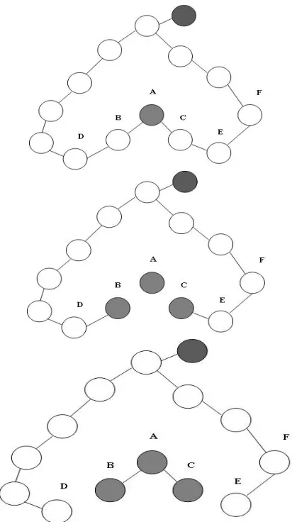
Fig 6 : Example of Shadow spread technique (a) Graph
contains concave node A (b) Disconnecting A from the graph, B and C becomes a concave node (c) After separating a sub graph consisted by A,B,C , there will be no conclave node in
the graph
In request to separate the first chart into shadow zones and bright nodes as appeared in Fig. 6(c), nodes ought to have the option to trade their status data (shadow/bright) alongside their area data. This data trade is acknowledged by intermittently communicating reference point messages that contain two fields: status and area. Each node on a chart ought to be ready to get the area data of the base station. In our system model, sensor nodes get the base station's area from it’s broadcast channel.
3.7COST–SPREADPROCEDURE
In view of the sub-graphs came about because of first (shadow-spread) stage, the second (cost-spread) stage starts. To outline this stage, we demonstrate a model in Fig. 7. At first every node on the diagram has a variable equivalent to its physical separation to the destination. We mark the variables on every node. In the initial step, each shadow node attempts to abstain from being encompassed by neighbors with larger variables. This is given in Fig 7(a).
Fig 7: Consider the shadow nodes as CH, TH & Sub ordinate
nodes
Fig 7(a) Shadow nodes A, B, C are determined
(b) Node A increases its cost to 22
3165
Fig 7 (C) Nodes B and C increases its cost due to mobility of nodes
Fig 7 (D) Node A increases its cost again into 28
As Fig. 7(b) appears, node A finds that every one of its neighbors have larger variables. To stay away from this circumstance, node expands its variable to 22 to be larger than the greatest expense of its neighbors by (Δ is set to 3 in this model). In the subsequent advance, nodes B and C locate that every one of their neighbors have larger variable (since node an expanded its variable). Because of this circumstance, they increment their variables to 25 and 24, separately, as Fig. 7(c) appears. This procedure finishes in the third step when node A builds it variable from 22 to 28, as appeared in Fig. 7(d).
Fig 7(E) All shadow nodes (A, B, C) are satisfied with their cost gradient from high to low cost
Presently, every shadow node (A, B and C) is fulfilled in light of the fact that they can at any rate discover a neighbor with a littler variable. We signify the variable kept up in every node as the expense. On the off chance that we provide every node a sending guidance to a neighbor following the high cost-to-low rule, as Fig. 7(e) appears, we build up ways over the entire chart to the base station. To make the procedure appeared in Fig. 7 conceivable, the cost data ought to be traded between nodes. Like status data utilized in the first (shadow spread) stage, this is acknowledged by adding the cost data to the intermittently communicated reference point messages. We should see that the procedure portrayed above is restricted in shadow regions rather than the entire system.
4.
SIMULATION
ANALYSIS
This simulation analysis has been directed utilizing NS3 modeler simulation. Be that as it may, NS3 is the best
simulation tool for differentiating the protocols, systems furthermore, advances especially in mobile network scenario. We simulate 100 nodes and 200 nodes for the simulation graph. The sensor nodes randomly deployed in 500 X 500 m area. The energy has been calculated in Joules. The comparative simulation analysis is carried with the existing protocols. The proposed work PPGA was compared with the above technique to get a better results. Likewise, it is intended to perform and dissect these innovations. The simulation has been done for various node to find the thickness. The energy consumption for load balancing has been measured by the unit Joules. In Fig. 7 the energy consumed for the various protocols has been analysed and compared with the mentioned time. In the above graph PPGA has the high energy level when compared with the other protocols. The packet delivery ratio will be maximum when compared with other protocols. The delivery of the nodes to the destination among the cluster region is very important.
Fig 7: Delivery Ratio of the nodes
3166 Fig 8: Collision rate of the nodes
Fig 9: Connection among the neighboring nodes and checking
delay status
In fig 9 the connectivity of the nodes has been mentioned clearly. In this paper the connectivity among the nodes plays a major role to reach the destination point. It helps to check the delay status of the nodes. The maximum delay of nodes leads to failure of connecting nodes. The proposed techniques delay of nodes will be minimum and the nodes can be connected
within the region in a successive manner.
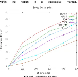
Fig 10: Consumed Energy
Fig 10 describes about the energy consumption of the nodes. The proposed technique consumes less energy to have a better network region. In the above diagram PPGA connect with the other nodes in a various above said methods. The node has been connected with other nodes through various techniques mentioned above. PPGA stands a good result in connecting with the nodes when compared with other protocols.
5.
CONCLUSION
In this paper, Partial Partitioned greedy Algorithm for Mobiles Sensor Networks (PPGA) is proposed. The Simulation results showed that the proposed algorithm PPGA performs better in terms of packet delivery ratio, collision rate, delay on nodes and energy consumption.
6.
REFERENCES
[1] J. Lian, K. Naik, and G. B. Agnew, ―Data capacity improvement of wireless sensor networks using non- uniform sensor distribution,‖ International Journal of Distributed Sensor Networks, vol. 2, no. 2, pp. 121–145, 2006.
[2] K. Ma, Y. Zhang, and W. Trappe, ―Managing the mobility of a mobile sensor network using network dynamics,‖ IEEE Transactions on Parallel and Distributed Systems, vol. 19, no. 1, pp. 106–120, 2008.
[3] C. E. Perkins and P. Bhagwat, ―Highly dynamic destination sequenced distance vector routing (DSDV) for mobile computers,‖ in Proceedings of the ACM Conference on Communications Architectures, Protocols and Applications (SIGCOMM ’94), pp. 234–244, 1994.
[4] Perkins, E. Belding-Royer, and S. Das, ―Ad hoc on demand distance vector(AODV) routing,‖ Tech. Rep. 3561, IETF MANETWorking Group, 2003.
[5] Alexandre Massayuki Okazaki and Antˆonio Augusto Fr¨ohlich ―ADHOP: an Energy Aware Routing Algorithm for Mobile Wireless Sensor Networks‖
Published 2012
https://www.semanticscholar.org/paper/ADHOP-%3A-an-3167 Energy-Aware-Routing-Algorithm-for-Okazaki-Fr%C3%B6hlich /
ff6066f2c01faf464d7fa5807cadeff7da720a2a
[6] Gianpaolo Cugola and Matteo Migliavacca ,‖ A Context and Content-Based Routing Protocol for Mobile Sensor Networks‖, European Conference on Wireless Sensor Networks EWSN 2009: Wireless Sensor Networks pp 69-85
[7] Xiaoxia Huang, Hongqiang Zhai and Yuguang Fang ―LIGHTWEIGHT ROBUST ROUTING IN MOBILE WIRELESS SENSOR NETWORKS‖ October 23 - 25, 2006, MILCOM'06 Proceedings of the 2006 IEEE conference on Military communications pages 2362-2367.
[8] Siming Li∗ Wei Zeng† Dengpan Zhou∗ David Xianfeng Gu∗ Jie Gao,‖ Compact Conformal Map for Greedy Routing in Wireless Mobile Sensor Networks‖ Dec 30, 2016
[9] Le Zou, Mi Lu, Zixiang Xiong,‖ PAGER-M: A Novel Location-based Routing Protocol for Mobile Sensor Networks ―2016, https://www.semanticscholar.org
[10]Shahzad Ali and Sajjad Madani,‖ Distributed Efficient Multi Hop Clustering Protocol for Mobile Sensor Networks‖, The International Arab Journal of Information Technology, Vol. 8, No. 3, July 2011