2009, 1–16, iFirst
Modal similarity
Ronaldo Vigo*
Cognitive Science Department, Indiana University at Bloomington, Bloomington, Indiana, USA
(Received 8 May 2007; final version received 4 February 2008)
Just as Boolean rules define Boolean categories, the Boolean operators define higher-order Boolean categories referred to asmodal categories. We examine the similarity order between these categories and the standard category of logical identity (i.e. the modal category defined by the biconditional or equivalence operator). Our goal is 4-fold: first, to introduce a similarity measure for determining this similarity order; second, to show that such a measure is a good predictor of the similarity assessment behaviour observed in our experiment involving key modal categories; third, to argue that as far as the modal categories are concerned, configural similarity assessment may be componential or analytical in nature; and lastly, to draw attention to the intimate interplay that may exist between deductive judgments, similarity assessment and categorisation. Keywords: similarity; modality; higher-order similarity; Boolean relational categories; Boolean metacategories; Boolean operators; modal categories
1. Introduction
In recent years, there has been renewed interest in the study of Boolean concepts (i.e. categories defined by Boolean rules): in particular, on how the formal properties of such categories account for their learnability (Feldman 2000; Vigo 2006; Lafond, Lacauture and Mineau 2006, Vigo 2008). The Boolean expressions or rules that define Boolean concepts are built with the building blocks of logic: namely, Boolean operators or logical relations such as conjunction, disjunction, equivalence, implication and exclusive-or. These operators are the ‘glue’ that keeps a set of objects bound as a category. Although they play a fundamental role in concept formation, categorisation, syntax and in reasoning, their cognitive roots have seldom been questioned. They remain abstract constructs of the highest order, able to organise our world in mysteriously fundamental ways, which prompt us to ask: What makes these Boolean relations so fundamentally important to our understanding of the world?
Like the Boolean relations, similarity relations have played a fundamental role in cognitive science. Indeed, long regarded as a core process of human cognition, similarity assessment has been central in understanding categorisation and object recognition behaviour. For example, similarity is the basis of Luce’s choice model of similarity (Luce 1952), the generalised context model of categorisation (Nosofsky 1984), and Shepard’s law of generalisation (Shepard 1987). More recently, it has been suggested
*Email: [email protected]
ISSN 0952–813X print/ISSN 1362–3079 online ß2009 Taylor & Francis
DOI: 10.1080/09528130802113422 http://www.informaworld.com
that similarity judgments may operate at multiple levels of comparative analysis. Under this view, categorisation and concept formation are processes mediated by similarity and dissimilarity comparisons at multiple levels of attention (Herrnstein 1990; Love 2000; Kroger et al., 2005). This is consistent with the view held by the analytic philosopher Rudolf Carnap (1928) who argued that abstract concepts could be derived from fundamental core experiences via the primitive formal relations of similarity and modality (the logical relations). In Carnap’s framework, similarity and logic combine to yield the primitive abstract relations necessary for forming higher-level concepts from our primitive experiences.
The connection between similarity and the logic operators is further enhanced by the fact that categorisation based on similarity judgments and on the construction of logical rules, both have been offered as core explanatory principles underlying human concept formation (Nosofsky, Palmeri and McKinley 1994). Perhaps more compelling is the fact that key models of similarity have relied on the the logical relations to do their work in the first place; most notable among these is Tversky’s (1977) model of similarity assessment based on the logic of sets. In what follows, we propose the inverse of this characterisation of similarity in terms of logic. We wish to show that the meaning of the Boolean operators themselves, the building blocks of Boolean logic and of Boolean concepts, is found in a similarity relation. One of the reasons why this is not an easy hypothesis to prove stems from the highly abstract meaning attributed to the connectives in the propositional calculus in the terms of either propositions (intensional entities) or truth values (extensional entities). Such representations may suffice for philosophical analysis but not for cognitive science.
Accordingly, to address this problem successfully, we follow the well-known approach of using Boolean expressions as Boolean rules that in turn define well-defined categories (Vigo 2006). This approach has been the staple of Boolean concept research and has led to a number of significant advancements in the field such as the SHJ learning difficulty ordering (Shepard, Hovland and Jenkins 1961) and the learning difficulty ordering of concepts defined by basic Boolean rules involving a single connective (Haygood and Bourne 1965). For example, in the latter research, Haygood and Bourne presented subjects with four dimensional stimuli and two focal attributes related by some rule unknown to the subjects. The rules tested were a conjunctive rule, a disjunctive rule, a conditional rule,
and a rule of joint denial (i.e. only objects that are neitheranorbare positive examples of
the concept). Subjects were then asked to identify the rule in question.
Subject performance was measured by the number of errors made before achieving 16 correct responses in a row. It was discovered that conjunctive rules were the least difficult to learn, followed by disjunctive rules, joint denial rules, and finally conditional rules. The result that disjunctive rules are more difficult to learn than conjunctive rules was consistent with a number of previous empirical findings: most notably those of Hunt and Hovland (1960), Welles (1963) and Conant and Trabasso (1964). Like in the work of these researchers, we identify Boolean constructs with categories. However, our approach differs in that the Boolean operators themselves, alone, define specific Boolean metacategories referred to as ‘modal categories’. As we shall see, there are only 16 possible types of modal categories corresponding to the sixteen possible binary Boolean operators. These are rich in structure and when compared to the standard category of logical identity (i.e. the modal category defined by the logical equivalence Boolean operator), they yield a clearly defined similarity order.
The layout of this article is as follows. Under Section 2, we introduce a representation of the modal categories as vectors of functions with two possible values. In Sections 3–5, we introduce a componential modal similarity measure on these representations that yields a degree of similarity for each modal category in respect to the standard category corresponding to logical equivalence. The approach taken here is one of step by step construction in the tradition of analytic philosophy. Section 6 of the article introduces the experimental paradigm used to test the predictions made by the measure. Also, it is here that we show that our model of modal similarity makes the correct empirical predictions. Based on our results, we propose that the logical connectives may be simply a shorthand for expressing degrees of modal similarity; these degrees correspond to different strengths of the conceptual ‘glue’ described above. This interpretation gives a highly plausible answer to why disjunctive concepts are more difficult to learn than conjunctive concepts. The answer is that disjunctive glue is weaker! Tacit to this point of view is the idea that deductive reasoning, and indeed other forms of human inference, may depend substantially on similarity assessment and categorisation. As such, we conjecture that language-based representations – such as propositions and truth-values – may not be necessary for deductive thought. Finally, in the conclusion we discuss some open problems and some suggestions for further research.
2. Modal categories
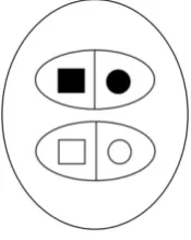
A modal category is a relational category or metacategory (i.e. a category of categories) consisting of up to four subcategories. Each subcategory contains a pair of objects and each object in each pair possesses or lacks a certain specified single feature. Figure 1 below illustrates a perceptual instance of the modal category described by the logical equivalence operator in respect to the feature ‘black’.
This category consists of two subcategories. In the first subcategory, we see two objects that bear a simple relation in respect to a pre-specified feature: namely, both objects are black. In the second subcategory, the same two objects bear a similar simple relation: namely, the colour black is absent from both. Together, these two subcategories form the modal relational category of logical equivalence since the relationship between its two subcategories is definable completely by the logical equivalence or biconditional operator. Recall that the biconditional operator assigns a value of true or 1 to two of four possible states: that is, when both objects (usually propositions) have the value true or 1, and when
Figure 1. Modal relational category (metacategory) in respect to the feature ‘black’ and corresponding to logical equivalence.
both objects (usually propositions) have the value false or 0. To the remaining two states of (1, 0) and (0,1), the equivalence operator assigns a value of false or 0.
More generally, a binary Boolean operator is a function from the cross product
O¼{1, 0}{1, 0}¼{(1, 1), (0, 0), (0, 1), (1, 0)} to the set {1, 0}. There is a total of 24ways
of assigning values to the four pairs in {1, 0}{1, 0}. Hence, there are 16 possible binary
Boolean operators. For example, the modal category in Figure 1 above is defined by the following function in extension (i.e. in terms of sets): {((1, 1), 1), ((0, 0), 1), ((0, 1), 0), ((1, 0), 0) }. By interpreting the pairs to which the function assigns a zero value (i.e. each pair of arguments with a zero next to it in the previous set) as the pair not being present in the category, we can further reduce this set to the set {(1, 1), (0, 0)}. These two pairs represent the two subcategories of the modal category of logical equivalence discussed above (Figure 1).
Using Boolean operators as descriptions of modal categories suggests that modal categories, and the objects comprising them, may be construed as functions from features to the modal states of presence and absence. This qualitative characterisation of a modal category will prove useful in defining our similarity measure. Thus, we shall say that
a stimulus-objectsis endowed – in respect to a specified attended property or feature’–
with a binary dimension of modality whose possible values areA(whenever the property or
feature is absent) and P (whenever the property or feature is present). For example,
suppose that the stimulus in question is a sphere and the property in question is the
property ‘red’. Letsstand for the sphere and’for the property ‘red’; then, the stimuluss
acts as a function on’ and is defined as follows:
sð’Þ ¼ Pif’ is present in respect tos
Aif’is absent in respect tos ð1Þ
In other words, when the sphere is red its modal dimension value isP (standing for the
property being present); whenever the sphere is not red, its modal dimension value is
A(standing for the property being absent). More generally, the modal dimension values of
a stimulus are those aspects of the stimulus that indicate, in respect to some property or feature, the presence or absence of that feature. This contextual (i.e. in respect to some property) definition characterises what it means for an object to be in a modal state in
respect to one of its possible features. Also, please note that’in the definition above could
be a set of features rather than a single feature, but for the purpose of our analysis and for
the sake of simplification,’ for the time being should be interpreted as a single feature.
Henceforth, we shall use the symbolsi(’) (where i2{A,P}) to denote the possible modal
dimension values or modal states ofs(’). For example,sA(’) means that’is absent insand
sP(’) means that’is present ins.
Under this representation of stimuli as functions, modal categories can be represented qualitatively by a vector of distinct pairs of modal values. Moreover, since the set C¼{(p
P(’),qP(’)), (pA(’),qA(’)), (pA(’),qP(’), (pP(’),qA(’))} of all possible distinct pairs of
modal values consists of four elements, then the power set of Cis the set of all possible
modal categories, 16 in total (2jCj
). These 16 are isomorphic to the Boolean operators as can be clearly seen from our definition of a Boolean operator above. For example,
E¼ h(pP(’),qP(’), (pA(’),qA(’))i is the vector representation of the modal category
corresponding to logical equivalence (Figure 1) since it stands for two-ordered pairs of
objects, one in which the feature’ is present in both objects (p andq) and the other in
which the feature’is absent in both stimuli.
A more succinct way of expressing this is by specifying the values of the functions
explicitly as follows: E¼ h(P,P), (A,A)i. Henceforth, we shall use upper case Greek
alphabet symbols as variables standing for the vector representations of modal categories and upper case Roman alphabet symbols as constants standing for vector representations
of specific categories. Lastly, for any modal category,(i) is theith pair of the modal
category(wherei2{1, 2, 3, 4}). If such a component does not exist in, then the value
of (i) is Ø. For example, forE¼ h(P,P), (A,A)i, E(1)¼(P,P), E(2)¼(A,A),E(3)¼Ø,
andE(4)¼Ø.
Now that we have a more natural formal representation of modal categories we proceed to define modal similarity. Modal similarity is the similarity relation between the
modal categories (24¼16 in total) and the logical categoryEof logical equivalence. But
why E as a prototype or standard? This stems from the assumption that similarity
measures purport to measure the degree of identity between two objects. But if these two objects are made of parts (as modal categories are), then the relationship between those parts should enter into the determination of overall similarity. Then, in essence, what we are comparing are relationships. We know that the equivalence operator expresses the
relation of logical identity. Thus, the relationship between the two subcategories of E
corresponds to the relationship of logical identity. In other words, by judging how similar
each modal category is toE, we are in effect determining the degree of logical equivalence
between their subcategories. As such, E is the ideal point for systematic comparison.
This will become clearer in the experimental section of this article.
Finally, it is important to recognise that the standard modal categoryEis not exactly a
prototype for similarity judgments. Prototype models are models in which exemplars are
compared to some central tendency value. In modal similarity theory, E is not a
central tendency but a high limit or absolute upper boundary representing maximal similarity among members of a Boolean metacategory. Likewise, the complimentary or
opposite logical category E0¼ h(p
P(’),qA(’)), (pA(’),qP(’))i (i.e. exclusive-or or negative
biconditional) ofErepresents the corresponding lower limit or absolute lower boundary
representing minimal similarity. Let us say that it is the 0 point of our scale. This way of
characterising the similarity relation is conceptually more along the lines of a bounded
prototypeorlimit prototypemodel of similarity.
3. A modal similarity measure
Next, we introduce a measure for determining the degree of similarity between any modal
category and the modal category E in respect to some property or feature ’.
Two features of our measure will stand out: first, its componential nature; second, the intimate interplay that similarity and dissimilarity plays at a lower level of comparative analysis. The measure depends on two primitive measures on the four basic pairs of items
(in setCabove) that define the contents of a modal category:
SimMðE;; ’Þ ¼fðsimpðpP;qPÞ;simpðpA;qAÞ;dispðpP;qAÞ;dispðpA;qPÞÞ ð2Þ
Here, the modal similarity SimM(E,,’) between the two modal categories E and in
respect to’ is a function of the values of two primitive partial measures simpand disp
(one similarity measure and one dissimilarity measure) on the four component pairs of the
modal category generated by the lower-order objectspandq(e.g. in Figure 1pandqare a
rectangle and a circle). Note that simp(pP,qP) above should have be written as
simp(pP,qP,’), and similarly for the other primitive measures. We have not specified’ to avoid extremely long equations.
Clearly, the ternary modal similarity measure SimM and the primitive measures are
functionals(i.e. functions from functions to scalars) since their arguments are objects or vectors of objects and in our framework objects are functions. The partial similarity
measure simp and the partial dissimilarity measure disp represent primitive similarity
judgments and primitive dissimilarity judgments consistent with our intuitions.
For example, when ’ is present in both stimuli agents should judge the highest degree
of modal similarity. It also seems reasonable that the next highest degree of primitive
modal similarity should be judged when’ is absent from both stimuli.
However, for the partial dissimilarity measure disp, whenever ’ is absent in p and
present inq we have a degree of modal dissimilarity that would seem to be equal to the
case where’is present inpbut absent inq. Nonetheless, the order of the stimuli must bear
on the dissimilarity measure since p and q are different objects. This assumption is
supported by numerous experimental results that suggest that human similarity assessment is not symmetric (Tversky 1977). In these experiments we find evidence that in going from the first stimulus to the second in a comparison task, the eventual presence of a property is less grounds for dissimilarity than its eventual absence. Thus, we assign the higher degree
of dissimilarity to disp(pA,qP) and the lower degree to disp(pP,qA).
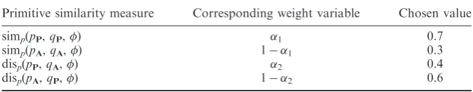
As is often done with similarity measures, we shall assign them a value in the real number interval [0, 1]. Furthermore, the two primitive similarity measures will be the
weights of the higher-order functionMedefined in (3) and (4) below. As such, they act as
two parameters1and2within our model. Intuitive values under the above criteria are
illustrated in Table 1 below.
Correspondingly, the first two weights contribute to a total similarity of 1, while the
other two contribute to a total dissimilarity of 1. Hence, the choice ofiand 1iin the
table. Next, we need to be able to describe within our formalism the presence or absence of
the four possible subcategories or pairs of objects that may make up a modal category.
We do so with the following higher-order functionMe:
e
Mðði;jÞÞ ¼ 1 ifði;jÞis present in
0 ifði;jÞis absent in ð3Þ
Or equivalently,
e
Mððsð’Þ;rð’ÞÞÞ ¼ 1 ifðsð’Þ;rð’ÞÞis present in
0 ifðsð’Þ;rð’ÞÞis absent in ð4Þ
The purpose of this higher-order function is to indicate and count the presence or absence of a particular subcategory in the modal category in question. A cognitive interpretation of this function is that modal similarity judgments involve metaprocessing.
Table 1. The four primitive similarity measures act as parameters at a lower level. Intuitive parameter values under our criteria are given below.
Primitive similarity measure Corresponding weight variable Chosen value
simp(pP,qP,) 1 0.7
simp(pA,qA,) 11 0.3
disp(pP,qA,) 2 0.4
disp(pA,qP,) 12 0.6
Now that we have the corresponding weights defined by our primitive similarity and dissimilarity relations, we see a broader picture of degrees of modal similarity as a function
of these two primitives. EachMewill act as a coefficient that determines which primitive
similarity and dissimilarity values should contribute to overall similarity. The following
formulation, where is a logical category, illustrates the role ofMe:
SimMðE;; ’Þ ¼simpðpPð’Þ;qPð’ÞÞMeðpPð’Þ;qPð’ÞÞ þsimpðpAð’Þ;qAð’ÞÞMeðpAð’Þ;qAð’ÞÞ
dispðpPð’Þ;qAð’ÞÞMeðpPð’Þ;qAð’ÞÞ dispðpAð’Þ;qPð’ÞÞMeðpAð’Þ;qPð’ÞÞ
ð5Þ
Or equivalently,
SimMðE;; ’Þ ¼simpðEð1ÞÞMeðEð1ÞÞ þsimpðEð2ÞÞMeðEð2ÞÞ
dispðE0ð1ÞÞMeðE0ð1ÞÞ dispðE0ð2ÞÞMeðE0ð2ÞÞ ð6Þ
By using the parameters 1 and 2 in place of the primitive similarity–dissimilarity
measures, we get the more succinct formula below:
SimMðE;; ’Þ ¼1MeðEð1ÞÞ þ ð11ÞMeðEð2ÞÞ 2MeðE0ð1ÞÞ ð12ÞMeðE0ð2ÞÞ
ð7Þ
But this function will not do. The measure must include an additional parameter
responsible for the relative emphasis of similarity over dissimilarity (as determined byMe,
E(k) andE0(k)). We select higher-order weights and 1 to compute the emphasis on
similarity or dissimilarity by an agent. The addition of such weights at a higher level makes the measure non-linear. This feature is consistent with experiments showing that in respect to relational comparisons, similarity and dissimilarity are not perfect compliments or linear inverses of each other (Medin, Goldstone, and Gentner 1990). In fact, our model provides a possible explanation for such lack of symmetry. Namely, that at a metacognitive processing level there is considerably more information to process (e.g. to compare), and that this change in complexity changes the character of the relationship between similarity and dissimilarity from linear to non-linear. Thus, with this additional modification to formula (7) above we get:
SimMðE;; ’Þ ¼½1MeðEð1ÞÞ þ ð11ÞMeðEð2ÞÞ
ð1Þ½2MeðE0ð1ÞÞ þ ð12ÞMeðE0ð2ÞÞ ð8Þ
One more definition is needed to finalise the construction of our modal similarity measure.
Modal categories whereE(1) is present are called positive modal categories. Accordingly,
modal categories where E(1) is not present are called negative modal categories.
The complements of the positive modal categories are the negative modal categories
and vice versa. For example, the positive modal category D¼ h(P,P), (P,A), (A,P)i
defined by the Boolean disjunction operator has the negative modal categoryD0¼ h(A,A)i
as its complement. Likewise, the positive modal category E¼ h(P,P), (A,A)i has the
negative modal categoryE0¼ h(P,A), (A,P)ias its complement. There are a total of eight
positive categories and eight negative ones. This leads us to the final assumption underlying our measurement. For complements of positive modal categories, i.e. for
negative modal categories, the 1 and 2 values for the primitive similarity and
dissimilarity measures are switched.
This means that when the modal category is negative, the difference between 1and
11 is greater for primitive dissimilarity than for primitive similarity. This seems
reasonable since the presence ofE(1) inshould contribute more to increasing the overall
judged similarity to Ethan its absence should contribute to lowering its overall judged
similarity toE. In turn, the presence ofE0(1) under the absence ofE(1) should subtract
more from our perceived overall similarity than its absence. In essence, these are contextual effects that will prove essential to the measure’s predictive performance. We invite readers to test for themselves the feasibility of this assumption by examining the experiment under Section 5. To account for this contextual property, Equation (7) above must be extended. This is accomplished by defining the measure as a step function in terms
of the absence or presence of E(1). Let b be the decimal representation of the binary
sequence hMeðpP;qPÞ;MeðpA;qAÞ;MeðpP;qAÞ;MeðpA;qPÞi, then we can finally define
modal similarity as follows:
SimMðE;; ’Þ ¼
½1MeðEð1ÞÞ þ ð11ÞMeðEð2ÞÞ
ð1Þ½2MeðE0ð1ÞÞ þ ð12ÞMeðE0ð2ÞÞ ifb2 f8;. . .;15g
½2MeðEð1ÞÞ þ ð12ÞMeðEð2ÞÞ
ð1Þ½1MeðE0ð1ÞÞ þ ð11ÞMeðE0ð2ÞÞ ifb2 f0;. . .;7g
Note that the order of the parameters1and2above have been switched, as planned, for
the second condition b2 f0;. . .;7g. This reverses the similarity and dissimilarity
primitives according to whether the modal category is positive or negative. We have listed this and other key assumptions underlying the above measure in the Technical Appendix at the end of this article.
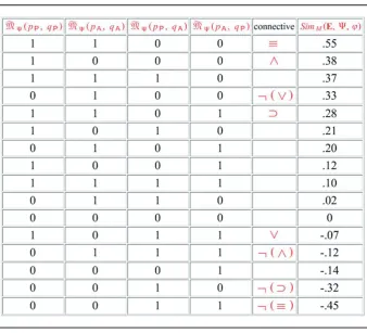
The degrees of modal similarity between stimuli for each of the 16 modal categories corresponding to the 16 Boolean operators in the propositional calculus can now be
computed. For example, when we let ¼0.55 (a slight emphasis on similarity over
dissimilarity), 1¼0.7, and 2¼0.4, we can generate the values shown in Table 2. This
slight emphasis is consistent with the idea that subjects have a bias towards modal similarity over modal dissimilarity comparisons. Note that the measure yields a linear order for the set of all 16 possible modal relations. This shows by construction that the linear completeness property (property 7 in the Technical Appendix) has been satisfied. If we look at each Boolean operator or logical connective in terms of the modal similarity measure assigned to the modal category that it defines, some interesting intuitive patterns emerge regarding their meaning: for one, conjunctions, implications and biconditionals may be regarded as expressing subsymbolically high degrees of modal similarity between stimuli, while disjunctions, and particularly ‘exclusive-or’ (equivalent to the negation of the biconditional connective), may be expressing subsymbolically low degrees of modal similarity. This seems to conform with the pragmatic notion that cognitive agents need to be able to express pronounced modal distinctions as well as pronounced modal likenesses in everyday life. More compelling is the connection to categorisation. Perhaps the reason why Boolean categories defined by disjunctive rules are more difficult to learn than conjunctive ones (Haygood and Bourne 1965) is because the categorical ‘glue’ provided by a disjunctive operator is weaker!
Those operators with modal similarity values that lie at the middle of the scale close to zero or neutrality, do not have much expressive power in this respect and consequently, may not play an overt role in natural language discourse. Second, the table confirms that
modal similarity is non-linear. These are but a few of the observations one may draw from this table; we leave it to other researchers to draw others. Regardless, the general representational approach introduced here for the modal categories and modal similarity can yield useful results by choosing appropriate values for the three discussed parameters as will be seen under the experiment under Section 5.
4. Comparisons to Tversky’s featural similarity measure
Clearly, our approach to measuring similarity judgments differs considerably from similarity distance measures that are dependent on representations of stimuli as
n-dimensional points in an n-dimensional psychological space (Shepard 1974). This
geometric approach is illustrated by Equation (10) below where n is the number of
dimensions in some psychological space,xpiis the value of theith dimension of stimulusp
andris a positive integer that allows for different spatial metrics. The Euclidean metric
(r¼2) is the best known of these.
Clearly, in these representations dissimilarity is measured by the sum of the distances (i.e. differences) between points across their dimensions. It has been convincingly argued by Shepard (1987) that subjective similarity is an inverse exponential function of this psychological distance. Perhaps the best known objection to this representational
Table 2. Modal similarity measure predictions when1¼0.55.
approach comes from Tversky (1977) who argues that the metric axioms on which the measure is based are not psychologically plausible. In addition, the measure does not account adequately for the very distinct contributions that similarity and dissimilarity comparisons between stimuli make to the total similarity measure.
dðp;qÞ ¼ X
n
i¼1
xpixqi
r
" #1=r
ð9Þ
In contrast, Equation (12) illustrates Tversky’s (1977) featural approach to measuring
similarity between stimuli. Here, objects are represented by sets of features P and Q.
By determining what the two sets have in common (i.e. their intersection) and determining
their differences, one can determine the overall degree of similarity between objects p
and q. In this formula, f is a function that assigns a number value to the set theoretic
expressions and i (i2{1, 2, 3}) are weights that adjust the degree of emphasis of the
measure of commonality and differences between sets.
Simðp;qÞ ¼1fðP\QÞ þ2fðPQÞ þ3fðQPÞ ð10Þ
But this approach, among other things, does not: a) yield a discriminating and meaningful result for sets with a single feature and b) capture the dynamic quality of the possible modal dimension values of stimuli in respect to attended features.
In contrast, our representation of stimuli as functions tacitly suggests the process of attention in the sense that modal similarity has no meaning unless it is defined contextually relative to the feature that is being attended to by the agent. In other words, our modal similarity relation is not a binary relation as in the above models, but a ternary one. In this respect, it has been argued by Goodman (1951) that the similarity relation only makes sense as a ternary relation, and as far as modal similarity is concerned, we tend to agree.
Some readers have probably wondered whether or not we can dispense with the introduced modal similarity measure by extending Tversky’s featural similarity measure. Such an extension is possible but only to the point where Tversky’s approach will no longer be recognised for what it is. In this section, I shall attempt such an extension to show its inadequacy. First, Tversky represents stimuli as sets of their features. Instead, in accordance with our aim, I shall substitute these sets of features with modal categories. In Tverky’s notation, we have the following measure.
SimðE;Þ ¼1fðE\Þ þ2fðEÞ þ3fðEÞ ð11Þ
If we letfbe the cardinality function (as is often done with this measure), this clearly will
not do since the measure then does not distinguish between the four modal pairs present or
absent in . Thus, it cannot assign unique values to them. Trying to remedy this by
defining some esoteric function f on sets, the measure would still not account for the
contextual effects induced by the complements of the modal categories. Finally, the use of set interception contributes nothing to the measure as is plainly apparent upon examination of the eight properties listed in the Technical Appendix.
However, we could be more inventive. Suppose instead that we modify the above
measure by including only two set operations, two functionssanddand the weightsand
1as seen below.
SimðE;Þ ¼X
x
sðx2 ½EÞ ð1Þ X
y
dðy2 ½EÞ ð12Þ
This formulation is far more promising. By definingsanddas functions that assign each
element ofEandEa specific value from {1, 11} and {2, 12}, respectively
(i.e. the values corresponding to the primitive similarity measure and the primitive dissimilarity measure defined in the previous section), the resulting measure is equivalent to our modal similarity measure minus the ability to account for negative modal categories. The obvious criticism here is that such a measure is not along the lines of what Tversky (1977) had intended in the first place.
5. The experiment
To determine the empirical similarity order of the key subset of the modal categories and to determine how well such an order is predicted by the similarity measure introduced in Section 3 above, we ran a simple perceptual experiment involving visual modal categories. In our experiment, we tested the modal categories corresponding to the commonly used Boolean operators: namely, equivalence, implication, conjunction, disjunction, exclusive-or and their negative counterparts or compliments.
5.1. Participants
A group of 25 undergraduate students from introductory psychology courses at Indiana University at Bloomington participated in the experiment. Subjects earned course credits for their participation. The data from an additional four participants were excluded for failure to follow the instructions adequately.
5.2. Apparatus
The experiment was conducted with the E-prime presentation software v. 2.0 (2005) running on a Dell Pentium 5 PC using a Dell 15’ LCD monitor.
5.3. Procedure
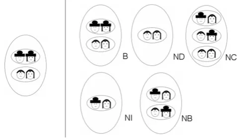
Prior to running the experiment, participants were given instructions on two screens. The first screen explained the comparison task. The second screen contained a specific example of the comparison task. The subjects were instructed to compare cultures in terms of the hat-wearing behaviour of marital couples. Each screen displayed a target culture to the left of a vertical line and five cultures to the right of the same line. The target culture was always that corresponding to the standard modal category defined by the logical equivalence operator. Four of the five cultures to the the right of the line were cultures corresponding to the positive modal categories defined by the following operators or connectives: implication, disjunction and conjunction, and as controls, the negative equivalence (i.e. exclusive-or) modal category and the equivalence or biconditional modal category.
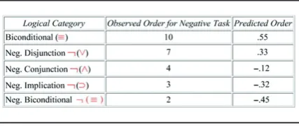
In addition to the positive task, a negative task was tested. Accordingly, for the
negative task, the five cultures to the the right of the line were cultures
corresponding to the negatives of the five modal categories displayed in the positive
task: negative implication, negative disjunction, negative conjunction, negative
equivalence and again as control the equivalence modal category. For both the positive and negative tasks, the subjects were asked to judge the degree of similarity between
each of the cultures to the right of the line to the target culture to the left of the line in terms of the hat-wearing behaviour of the cultures (i.e. on whether or not a hat was present on the head of a male or a female for the sets of marital couples). Subjects were asked to make the comparison on a scale from 1 to 10, 1 being least similar and 10 being identical. Figures 2 and 3 above show sample screens of the positive and negative tasks.
Figure 2. Experimental Display for the common positive modal categories: B stands for biconditional, C stands for conjunction, I stands for implication, D stands for disjunction and NB stands for negative biconditional or exclusive-or. The B and NB modal categories were used as controls in this positive set. These labels were not present in the actual displays seen by subjects.
Figure 3. Experimental Display for the common negative modal categories: B stands for biconditional and serves as a control, ND stands for the negative of the disjunction NC stands for the negative of the conjunction, NI stands for the negative of implication, and NB stands for the negative of the biconditional or exclusive-or. These labels were not present in the actual displays seen by subjects.
Subjects were presented with 20 trials of the positive tasks and 20 trials of the negative tasks where the order of the cultures was displayed at random in each trial. Also, for each trial the pairs of marital couples were permuted randomly within each culture. Subjects were asked to enter their responses using a prompt located at the lower left hand side of the screen. Furthermore, they could edit their entries in order to correct mistakes before moving to the next trial.
5.4. Results and discussion
We assessed the underlying similarity ordering by taking the average responses for the 20 positive trials and the 20 negative trials. The similarity ordering for the tested logical categories is given in Tables 3 and 4 above. Since in the experimental paradigm the positive and negative tasks were given separately, we obtained two separate orders: one for the positive logical categories and one for the negative logical categories. As can be seen in Tables 3 and 4 above, both orders are predicted by the modal similarity measure
introduced in Section 3. The parameters1¼0.7,2¼0.4, and1¼0.55 chosen earlier in
our theoretical discussion turned out to be the correct ones to make these predictions. These values are seen also in Table 2 under Section 3 above.
6. Conclusions and future research
We have proposed a modal similarity measure for simple key metacategories defined by the Boolean operators. The proposed similarity representation differs from geometric and featural representations in several ways: first, stimuli are represented as functions into two possible modal-dimensions or modal states of presence or absence. Second, the representation is componential in nature. This kind of parameterised component model of similarity, as far as we know, is new to the literature. Its design is consistent with the
Table 3. Predictions for positive logical categories.
Table 4. Predictions for negative logical categories.
hypothesis that similarity judgments are the result of compounding lower-level similarity judgments based on modal aspects of the pair of stimuli. Third, our modal similarity measure is a functional from vectors to real numbers rather than a function. Fourth, similarity and dissimilarity are treated as separate and competing contributors to the similarity judgment process. Fifth, the measure, as a ternary relation, suggests selective attention processes in that it defines similarity relative to a feature or a set of features
(i.e. ‘is similar toEin respect to’’).
Another unique aspect of the proposed measure is that it derives a degree of similarity
for each of the logical categories not as a value within [0, 1] but as a value within [1, 1].
We feel that this is the correct choice since it stresses the importance of treating similarity and dissimilarity as independent contributors to total similarity (or more accurately, total ‘collation’). Moreover, the resulting similarity order for the modal categories also conformed to our intuitions regarding the well-known Boolean operators that define them. More specifically, if we think of Boolean operators as expressions of degrees of modal similarity, then this would explain why some are more useful than others in daily discourse. This hypothesis can have a great impact on categorisation. As mentioned, it might explain why Boolean categories defined by disjunctive rules are more difficult to learn than conjunctive ones (Haygood and Bourne, 1965). The answer, according to our model, is simple: the categorical glue (modal similarity) provided by a disjunctive operator is much weaker!
As importantly, the proposed model of similarity was able to predict the empirical similarity order for the key modal categories. These are key categories in that they correspond to the most widely used connectives. A possible extension of this research is to determine an empirical order for the remaining modal categories and see whether or not the proposed model can predict this larger order as well. Notwithstanding the success of our measure, we attempted to extend Tversky’s (1977) featural similarity measure to accommodate the modal categories. Although after considerable manipulation of some fundamental ideas, we were able to obtain a measure equivalent to our modal similarity measure, it bore little or no resemblance to Tversky’s original measure.
Although we restricted our discussion to objects possessing a single property or feature, the theory can be easily extended to objects possessing a finite number of properties or features. This extension is interesting since it can provide a more robust link to the role that attention processes may play in modal similarity judgments. Another possible research direction is to extend the measure so that it can predict the similarity order of other types of metacategories beyond those defined by Boolean operators: for example, such as those obtained by increasing the number of objects in the modal category from two to three and beyond. These scenarios are worth exploring from the standpoint of a theory of combined ‘atomic measures’ relative to each feature in the set of relevant features. Such a theory could help establish the desired link between similarity-based categorisation and categorisation based on logical rules by the systematic decomposition of rules into atomic similarity components.
In conclusion, there seem to be aspects of similarity that are still uncharted and that conceptually fall somewhere between the widely-known featural and dimensional approaches to similarity. Central to these uncharted aspects are the notions of higher-order dimensions (e.g. modal dimensions), lower-level components of relational or metacatego-rical stimuli, and modal categories. Meanwhile, it is hoped that the questions raised in this article as well as their proposed solutions pave the way and shed some light on the cognitive nature of the logical operators and on the nature of configural similarity.
Acknowledgements
I would like to thank John Krusche for his helpful advice regarding my experiment. I would also like to thank Robert Nosofsky for his continued support throughout this project and Colin Allen, James Townsend and Robert Goldstone for their helpful comments and suggestions. This article is dedicated to the memory of my advisor, Alonzo Church. This research was supported in part by National Institute of Mental Health Grant R01MH48494.
References
Carnap, R. (1928),Der Logische Aufbau der Welt. Leipzig: Felix Meiner Verlag. (Rolf A. George, 1967, English trans.), The Logical Structure of the World. Pseudoproblems in Philosophy, Berkeley and Los Angeles, CA: University of California Press.
Conant, M.B, and Trabsso, T. (1964), ‘Conjunctive and Disjunctive Concept Formation under Equal-information Conditions’,Journal of Experimental Pychology, 67, 250–255.
Feldman, J. (2000), ‘Minimization of Boolean Complexity in Human Concept Learning’,Nature, 407, 630–633.
Medin, D.L., Goldstone, R.L., and Gentner, D. (1990), ‘Similarity Involving Attributes and Relations: Judgments of Similarity and Difference are not Inverses’, Psychological Science, Research Report, 1(1), 64–69.
Goodman, N. (1951),The Structure of Appearance, Cambridge, MA: Harvard UP.
Haygood, R.C., and Bourne Jr., L.E. (1965), ‘Attribute-and-rule Learning Aspects of Conceptual Behaviour’,Psychological Review, 72, 175–195.
Herrnstein, R.J. (1990), ‘Levels of Stimulus Control: A Functional Approach’,Cognition, 37, 133–166. Hunt, E.B., and Hovland, C.I. (1960), ‘Order of Consideration of Different Types of Concepts’,
Journal of Experimental Psychology, 59, 220–225.
Kroger, J., Holyoak, K., and Hummel, J. (2004), ‘Varieties of Sameness: The Impact of Relational Complexity on Perceptual Comparisons’,Cognitive Science Journal, 28(3), 335–358.
Lafond, D., Lacouture, Y., and Mineau, G. (2006), ‘Complexity Minimization in Rule-based Category Learning: Revising the Catalog of Boolean Concepts and Evidence for Non-minimal Rules’,Journal of Mathematical Psychology, 51(2), 57–74.
Love, B.C. (2000), ‘A Computational Level Theory of Similarity’, inProceedings of the Cognitive Science Society, USA, 22, pp. 316–321.
Luce, R.D. (1959),Individual Choice Behavior: A Theoretical Analysis, New York: Wiley.
Nosofsky, R.M. (1984), ‘Choice, Similarity, and the Context Theory of Classification’,Journal of Experimental Psychology: Learning, Memory, and Cognition, 10, 104–114.
Nosofsky, R.M., Palmeri, T.J., and McKinley, S.C. (1994), ‘Rule-plus-exception Model of Classification Learning’,Psychological Review, 101(1), 53–79.
Shepard, R.N. (1974), ‘Representation of structure in similarity data: Problems and prospects’, Psychometrika, 39(4), 373–422.
Shepard, R.N. (1987), ‘Toward a universal law of generalization for psychological science’,Science, 237, 1317–1323.
Shepard, R., Hovland, C.L., and Jenkins, H.M. (1961), ‘Learning and Memorization of Classifications’,Psychological Monographs: General and Applied, 75(13), 1–42.
Tversky, A. (1977), ‘Features of Similarity’,Psychological Review, 84(4), 327–352.
Vigo, R. (2006), ‘A Note on the Complexity of Boolean Concepts’, Journal of Mathematical Psychology, 50, 501–510.
Vigo, R. (2008), ‘Categorical Invariance and Structural Complexity in Human Concept Learning’, Journal of Mathematical Psychologyin press.
Welles, H. (1963), ‘Effects of Transfer and Problem Structure in Disjunctive Concept Formation’, Journal of Experimental Psychology, 65, 63–69.
Technical Appendix
Modal similarity analytic postulates
Please note that the following analytic postulates are not meant as the basis for an axiomatic representation theory of modal similarity; instead, they are meant to summarise
the basic assumptions underlying the modal similarity measure. Below,E¼ h(pP(’),qP(’)),
(pA(’),qA(’))i,is a modal category, and’is a property or feature. (Readers should refer
to section 3 of this manuscript for a detailed explanation of the rest of the notation used below.)
(1) Existence Property I (of Primitive Similarities and Dissimilarities). For any pair of
objects p and q there exist two primitive modal similarity measures and two
primitive modal dissimilarity measures from which our total measure will be
derived: namely, simp(pP(’),qP(’)), simp(pA(’),qA(’)), disp(pP(’),qA(’)), and
disp(pA(’),qP(’)). These two measures are real-valued functions between zero and
one that satisfy postulates 3 and 4 below.
(2) Compositional Property. Total modal similarity is a real-valued function of
primitive similarity and dissimilarity: SimM(E,,’)¼f(simp(pP(’),qP(’)),
simp(pA(’),qA(’)), disp(pP(’),qA(’)), disp(pA(’),qP(’)))
(3) Order Property. The primitive similarity and dissimilarity measures are ordered
as follows: simp(pP(’),qP(’))4simp(pA(’),qA(’)) and disp(pA(’),qP(’))4
disp(pP(’),qA(’))
(4) Summation Postulate. Partial similarity adds up to 1 and partial dissimilarity
adds up to 1: simp (pP(’),qP(’))þsimp(pA(’),qA(’))¼1; disp(pP(’),qA(’))þ
disp(pA(’),qP(’))¼1
(5) Maximal and Minimal Modal Similarity Property. Maximal and minimal
similarity values for the modal similarity measure are given by:
Max(SimM(E,,’))¼SimM(E,E,’) and MinðSimMðE;; ’ÞÞ ¼SimM E;E; ’
whereE¼ h(pP(’),qA(’)), (pA(’),qP(’))i.
(6) Zero Property. The modal similarity value for the empty vector h i or Ø is zero:
SimM(E, Ø,’))¼0.
(7) Contextual Reversal Property. Suppose that simp(pP(’),qP(’))¼1and disp(pP(’),
qA(’))¼2 if E(1)2, then simp(pP(’),qP(’))¼2 and disp(pP(’),qA(’))¼1 if
E(1).
(8) Existence Property II (of metafunction Me). For any pair of modal dimensional
values (p(’),q(’))2{(pP(’),qP(’)), (pA(’),qA(’)), (pP(’),qA(’)), (pA(’),qP(’))}, there
exists a metafunctionMe such that:
e
Mððpð’Þ;qð’ÞÞÞ ¼ 1 ifðpð’Þ;qð’ÞÞis present in
0 ifðpð’Þ;qð’ÞÞis absent in
Please note that postulate 6 simply states that the empty modal relation Ø expresses neither a degree of similarity nor a degree of dissimilarity: this means that in some sense it expresses ‘‘comparative’’ neutrality – or perhaps better yet, it expresses nothing in respect to similarity or dissimilarity. Postulate 7 simply states that the measure must do what we expected it to do: namely, to assign to each modal category corresponding to each of the logical connectives a unique degree of modal similarity.
In the appendix, postulate 7 has a proper subset symbol where there should be a "not an element of" symbol. Also, the sentence before equation 10 on page 10
was mistakenly truncated by the typesetter. It should say: "...and differences between sets, where the parameters alpha 2 and alpha 3 are negative real numbers."
These errors were introduced by the typesetter.