Modeling and Detecting Gravitational Waves from Compact Stellar Objects

(1)

Modeling and Detecting Gravitational Waves

from Compact Stellar Objects

Thesis by

Michele Vallisneri

In Partial Fulﬁllment of the Requirements

for the Degree of

Doctor of Philosophy

California Institute of Technology

Pasadena, California

2002

(2)

c

2002

Michele Vallisneri

(3)

Acknowledgements

As I sit down to write these acknowledgments, I realize what a happy journey the last four years

have been, how many special and talented people I have met here at Caltech, and how many equally

special people have supported me from afar. I am so lucky!

So, ﬁrst of all, I wish to thank Kip Thorne, who has been everything that an advisor can be,

and more. I hope I can live up to his enthusiastic and painstaking eﬀorts to teach me, mostly by

example, how to be a good scientist, how to do sound, thorough and timely research, how to live in

the scientiﬁc community, and how to write clear English prose.

Kip is ﬁrst, but during these years I have had other wonderful teachers. I thank Lee Lindblom

for our daily chats: I never came away from them without learning something new. I thank Joel

Tohline for introducing me to the wonderful world of numerical simulations, and for being a perfect

host on my visit to Baton Rouge. I thank Massimo Pauri for his unfailing support of my American

adventure, and for revealing to me the charm and surprise of spacetime physics. Of the other Caltech

faculty that I had the good luck of interacting with, I wish to thank in particular Tom Prince, Ken

Libbrecht, Marc Kamionkowski, Roger Blandford, and Sterl Phinney.

Alessandra Buonanno was a precious collaborator and a valued friend. I am thankful to her, and

to Yanbei Chen, for the tremendous nonstop effort they put into the final rush to finish Chap. 4 of

this thesis. As one point, I would work in the morning, Alessandra would elaborate on my output

during the afternoon, and make lists of things for Yanbei to do at night. At Caltech research can

truly be a 24/7 endeavor!

For support, inspiration, friendship and useful discussions (in any combination), I thank also

C. Alabiso, B. Allen, L. Bildsten, L. Blanchet, L. Burko, M. Casartelli, D. Chernoﬀ, G. M. Cicuta,

R. Co¨ısson, J. Creighton, C. Cutler, E. D’Ambrosio, T. Damour, R. De Pietri, J. Frank, J.

Fried-man, S. Gon¸calves, G. Gonzalez, V. Kalogera, D. Kenneﬁck, A. Lazzarini, L. Lehner, Yu. Levin,

G. Mambriani, J. Mason, D. Meier, E. Onofri, M. Ortaggio, B. Owen, F. Piazza, R. Price, J. Pullin,

C. Rovelli, B. Sathyaprakash, M. Scheel, A. Scotti, N. Stergioulas, K. Strain, L. Superchi, M. Tinto,

G. Ushomirsky, A. Vicer`e, and everybody else that I forget about now.

For kindling my love of the English language, and for helping me conceive and realize the dream

(4)

I wish to thank also all the fellow Tapirs of the last four years, and in particular the other Kiplings,

Kashif Alvi (a true friend if there is one), Mihai Bondarescu, Teviet Creighton, Scott Hughes, Patricia

Purdue, Yuk Tung Liu, and Richard O’Shaughnessy. We have shared many scientiﬁc discussions

and many nonscientiﬁc ones. I loved both kinds.

For making my life in California much happier and fuller that it could have been otherwise, I

thank all the wonderful friends I met here, and in particular my trio of pals, Alexei, Ed and Jason;

and then Tina, Andrew, Rob, Bill (especially Bill!), and all the Phys. Rev. Netters. My roommate

Mika was a lot of fun to live with, and an inexhaustible resource on literally any computing machine

ever made or conceived.

Chris Mach was a friend and a teacher; he taught me system administration and he fed me

garlic breadsticks with Alfredo sauce. What more can you ask? Shirley Hampton, Donna Driscoll

and Jo-Ann Hasbach always joined their utmost professionality with the warmest welcoming smile.

Jo-Ann Ruﬀolo’s advice was perhaps the strongest element in my favor during my job search; and

her kindness andjoie de vivre were always refreshing in the middle of that otherwise anxiety-ridden

process.

My thanks a my love go to my family, back in Italy (Dad, Mom, Cecilia, my aunts Alberta and

Maria, my mother-in-law Vittoria and brother-in-law Francesco) and here in the States (Ted and

Mada). Finally, thanks to my best men, faithful friends, and fellow travelers through life, Kola and

Filippo. All that is gold does not glitter, not all those who wander are lost.

Last but most important of all, I thank my love, Elisa, for being always on my side, for marrying

me, and for making my life happier every day. It is possible that this thesis might have been

completed even without her—but it would have been a joyless and somber exercise.

Now for the institutional acknowledgments: I thank CACR for access to the HP V2500 computers

at Caltech, where the primary simulations featured in Chap. 3 were performed; Mark Bartelt in

particular was always very helpful. Through the years, this research was supported by NSF grants

AST-9731698, AST-9987344, PHY-9796079, PHY-9900776, PHY-9907949, and PHY-0099568, and

by NASA grants NAG5-4093 and NAG5-8497, and NAG5-10707. I thank also Caltech for awarding

me a Special Institute Fellowship during my ﬁrst year of graduate school, and the PMA Division for

(5)

Abstract

In the next few years, the ﬁrst detections of gravity-wave signals using Earth-based

interferomet-ric detectors will begin to provide precious new information about the structure, dynamics, and

evolution of compact bodies, such as neutron stars and black holes, both isolated and in binary

systems. The intrinsic weakness of gravity-wave signals requires a proactive approach to modeling

the prospective sources and anticipating the shape of the signals that we seek to detect. Full-blown

3-D numerical simulations of the sources are playing and will play an important role in planning

the gravity-wave data-analysis eﬀort. This thesis explores the interplay between numerical source

modeling and data analysis, looking closely at three case studies.

1. I evaluate the prospects for extracting equation-of-state information from neutron-star tidal

disruption in neutron-star–black-hole binaries with LIGO-II, and I estimate that the

obser-vation of disrupting systems at distances that yield about one event per year should allow

the determination of the neutron-star radius to about 15%, which compares favorably to the

currently available electromagnetic determinations.

2. In collaboration with Lee Lindblom and Joel Tohline, I perform numerical simulations of the

nonlinear dynamics of the r-mode instability in young, rapidly spinning neutron stars, and I

ﬁnd evidence that nonlinear couplings to other modes will not pose a signiﬁcant limitation to

the growth of ther-mode amplitude.

3. In collaboration with Alessandra Buonanno and Yanbei Chen, I study the problem of detecting

gravity waves from solar-mass black-hole–black-hole binaries with LIGO-I, and I construct two

families ofdetectiontemplates that address the inadequacy of standard post-Newtonian theory

(6)

List of Figures

2.1 Plot of noise spectral density for diﬀerent LIGO conﬁgurations . . . 24

2.2 NS radiusR vs. disruption-onset frequencyftd, form= 1.4M andM = 2.5–80M. 26 3.1 Evolution of ther-mode amplitude in a slowly rotating star . . . 39

3.2 Real and imaginary parts of the current multipole momentJ22for run C1 . . . 40

3.3 Frequency of them= 2 r-mode for run C1 . . . 41

3.4 Numerical evolution of ReJ22 in production run C3 . . . 42

3.5 Numerical evolution of ther-mode amplitudeαin production run C3 . . . 42

3.6 Evolution of total mass, total angular momentum, and total kinetic energy in produc-tion run C3 . . . 43

3.7 Theoretical and numerical evolution of the total energy in production run C3 . . . 44

3.8 Isodensity surfaces showing breaking waves near the end of production run C3 . . . . 45

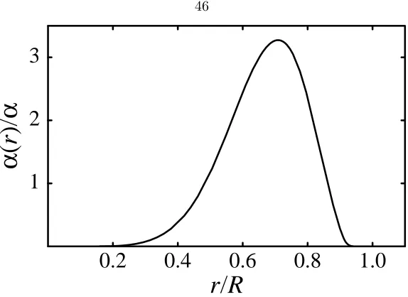
3.9 Radial amplitude densityα(r) of them= 2r-mode in production run C3 att= 22.5P0 46 3.10 Evolution of the phase-coherence function ∆φ in production run C3 . . . 47

3.11 Numerical evolution of ther-mode frequencyω in production run C3 . . . 47

3.12 Numerical evolution of the average stellar angular velocity ¯Ω in production run C3 . . 48

3.13 Numerical evolution of the diﬀerential rotation ∆Ω in production run C3 . . . 49

3.14 Meridional structure of the diﬀerential rotation in production run C3 . . . 49

3.15 Numerical evolution of the mass momentQ32 and of ther-mode amplitudeαin pro-duction run C3 . . . 52

3.16 Numerical evolution of ther-mode amplitudeαin low-resolution run C3* and in run C3 55 3.17 Numerical evolution of ther-mode amplitudeαin production runs C3–C5 . . . 57

3.18 Numerical evolution of ther-mode frequencyω in production runs C3–C5 . . . 57

3.19 Numerical evolution of the diﬀerential rotation ∆Ω in production runs C3–C5 . . . . 58

3.20 Numerical evolution of ther-mode amplitudeαin production runs C6–C8 . . . 59

3.21 Numerical evolution of ther-mode frequencyω in production runs C6 and C7 . . . . 60

3.22 Numerical evolution of the diﬀerential rotation ∆Ω in production runs C6–C8 . . . . 60

3.23 Numerical evolution of ther-mode amplitudeαin the extended run C4 . . . 62

(10)

3.25 Diﬀerential rotation ∆Ω through the extended run C4 . . . 63

3.26 Meridional structure of diﬀerential rotation at the end of production run C4 . . . 64

4.1 Square root of the noise spectral densitySn(f) for LIGO-I and VIRGO . . . 83

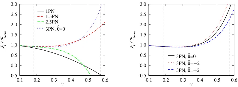
4.2 (i) Normalized flux functionFT_N/FNewt at various PN orders for η= 0.25. (ii) Effect of the parameterθon the normalized flux function at 3PN and 3.5PN orders . . . 85

4.3 (i) Energy functionET_N at diﬀerent PN orders forη= 0.25. (ii) Percentage diﬀerence in the energy function at the LIGO-I peak-sensitivity GW frequency . . . 86

4.4 Frequency-domain amplitude for T models at diﬀerent PN orders . . . 89

4.5 (i) Normalized flux functionFP_N/FNewt at different PN orders. (ii) Percentage differ-ence in the flux function between the T- and P-approximants . . . 90

4.6 (i) Energy functionEP_N at diﬀerent PN orders. (ii) Percentage diﬀerence in the energy function between 2PN and 3PN P-approximants . . . 91

4.7 Percentage diﬀerence between T- and P-approximants to the energy function, at the LIGO-I peak-sensitivity GW frequency . . . 93

4.8 Frequency-domain amplitude for the P models . . . 94

4.9 Frequency-domain amplitude of the HT and HP models . . . 97

4.10 Frequency-domain amplitude of the EP models . . . 104

4.11 Binding energyE(v) for equal-mass BBHs . . . 105

4.12 Signal-to-noise ratio at 100 Mpc versus total massM for selected PN models . . . 106

4.13 Iso-match contours for the functionh(ψ0, ψ3/2), h(ψ0+ ∆ψ0, ψ3/2+ ∆ψ3/2); values of ∆fcut(versusfcut) required to obtain matchesh(fcut), h(fcut+ ∆fcut)of 0.95, 0.975 and 0.99. . . 110

4.14 Projection of the ET(2,5/2) waveforms onto the frequency-domain detection template space . . . 111

4.15 Projection of the PN waveforms onto the Fourier-domain detection templates . . . 113

4.16 Projection of PN waveforms onto the P(2,5/2) detection template space . . . 119

4.17 Projection of PN waveforms onto the EP(3,7/2) detection template space . . . 120

(11)

List of Tables

1.1 Qualitative summary of the Newtonian simulations of NS tidal disruption in NS–BH

binaries . . . 9

1.2 Estimated coalescence and detection rates for compact binaries . . . 15

2.1 Fractional uncertainty ∆R/R, averaged over the range 10 km< R <15 km . . . 28

3.1 Physical parameters for the equilibrium models . . . 38

4.1 Location of the MECO for T-approximants . . . 87

4.2 Cauchy convergence of the T-approximants . . . 87

4.3 Location of the MECO for P-approximants . . . 91

4.4 Cauchy convergence of the P-approximants . . . 92

4.5 Cauchy convergence of the HP-approximants . . . 96

4.6 Fitting factors for the projection of the L model onto several PN models . . . 99

4.7 Location of the ISCO for the EOB-improved Hamiltonian . . . 101

4.8 Cauchy convergence of the EP-approximants . . . 102

4.9 End-to-end matches and number of templates (for MM0.98) along the mass lines of Fig. 4.15 . . . 112

4.10 Ranges for the ending frequencies of PN waveforms along the mass lines of Fig. 4.15 . 114 4.11 Estimation of the chirp massesMfrom the projections of the PN target models onto the Fourier-domain detection template space . . . 117

4.12 Fitting factors between T and ET models, at 2PN and 3PN orders . . . 124

4.13 Fitting factors for the projection of EP(3,7/2,0) templates onto themselves, for various choices of the parametersz1 andz2 . . . 125

4.14 Fitting factors between several PN models, at 2PN and 3PN orders . . . 126

4.15 Fitting factors for the projection of the target models onto the Fourier-domain detection template family . . . 127

(12)

4.17 Fitting factors for the projection of the target models (in the rows) onto the EP(3,7/2,0)

(13)

Chapter 1 Introduction

In the course of the next decade, the inception of gravity-wave (GW) astronomy will open an

exciting new window on the physics of compact, strongly gravitating bodies, such as neutron stars

(NSs) and black holes (BHs), both as isolated objects and in binaries; it will provide information

complementary to that available from electromagnetic and neutrino observations; and it will produce

important insights into unsolved questions such as the equation of state (EOS) of matter at nuclear

densities, the evolutionary channels that create NSs and BHs, and the mechanisms behind

gamma-ray bursts.

Meanwhile, sophisticated three-dimensional numerical simulations of GW sources are coming

of age, allowing unprecedented investigations into the eﬀect of the internal dynamics of compact

objects on their GW emission, and slowly but surely moving toward the goals of modeling the fully

relativistic dynamics of close and merging NS and BH binaries. Learning to interface numerical

simulations with other general-relativistic approximation techniques and with the GW data-analysis

algorithms will be of paramount importance as detector data become available. At the same time,

the theory of GW detection and data analysis has become ﬁrmly established as a mature subﬁeld

of GW science. Yet the very sources that arguably give us our best chance of detecting GWs in the

ﬁrst ground-based searches (binary BHs with total mass∼10–40M) lie at the very boundary of

the current data-analysis capabilities.

The interplay between analytical and numerical source modeling and data analysis is the

un-derlying theme of this thesis. Chapter 2 and (brieﬂy) Sec. 1.1.2 below deal with the prospects for

extracting EOS information from NS tidal-disruption waves. Chapter 3 and Sec. 1.1.3 below

dis-cuss the numerical simulations of the NSr-mode instability that I have completed in collaboration

with Lee Lindblom and Joel Tohline. Finally, Chapter 4 and Sec. 1.2.2 below report my work (in

progress, and in collaboration with Alessandra Buonanno and Yanbei Chen) on providing detection

(14)

1.1 Gravitational waves as a probe into the structure and

dynamics of neutron stars

Neutron stars are truly wondrous objects. They pack the mass of our Sun within diameters of 20–30

km; and they manage to be both a bona ﬁde test case for the theory of general relativity, and a

laboratory for the physics of matter at extreme density and temperature. Although more than a

thousand NSs are known today from electromagnetic observations (most of them detected as radio

pulsars), the ﬁrst GW detections of these objects are eagerly awaited.

1.1.1 Neutron stars as GW sources

Detailed reviews of GW sources, of the expected event rates, and of the physics that these sources

could teach us are available elsewhere [1, 2, 3]. Here I shall list brieﬂy the most promising types of

astrophysical systems from which we could learn about NSs using ground-based GW interferometers,

such as LIGO and VIRGO.

1. NS–NS and NS–BH binaries in the last few minutes of their inspirals. For a long time, these

inspiraling systems have been the prototype for the category of short-lived chirp signals

de-tectable using ground-based interferometers. The reason, of course, is that NS–NS binaries

have actually been observed in our galaxy [4], but also that the part of the inspiral accessible

to the interferometers (with GW frequencies between 40 and 1000 Hz) sits well before the ﬁnal

merger of the binary, so it is described very accurately by the well-developed post-Newtonian

equations for point masses (see Chap. 4). The successful observation of GWs from these

in-spirals will teach us about the masses, spins and locations of NSs, but not about their internal

structure.

By contrast, the detection of GWs from the endpoint of NS–BH inspirals should produce

detailed information about NS structure and EOS. For a wide range of binary parameters, the

NS will be torn apart by the tidal ﬁeld of the BH well before the ﬁnal plunge into the hole,

and the tidal-disruption waves will be well inside the frequency range of good interferometer

sensitivity. NS–BH binaries have also been proposed as engines for gamma-ray bursts [5] and

as suitable environments for the production of heavy nuclei in r-processes [6]. These systems

are the subject of Sec. 1.1.2 and Chap. 2. The expected measured-event rates are shown in

Table 1.2 and discussed brieﬂy in Sec. 1.2.1.

2. Rapidly spinning, deformed NSs. This class includes the known and unknown pulsars (when

their gravitational ellipticity is high enough to provide strong GWs), and the systems known

as low-mass X-ray binaries (LMXB), where the NS is accreting matter and angular momentum

(15)

3 ms; it is conjectured that the angular momentum being accreted is lost to the emission of

GWs [7].

To detect rapidly spinning NSs, it will be necessary to integrate the GW signal for times up to

several months, so the Doppler frequency modulations caused by the earth’s spin and motion

(both around the Moon and the Sun) will make it much harder to detect previously unknown

sources [8]. At the same time, the shapes of these modulations will make it possible to obtain

the position of the source in the sky [9], and in some cases to match the GW source with one

of the objects known from electromagnetic observations.

If any GWs are detected from spinning NSs, their features will be very informative, in particular

when examined in correlation with electromagnetic signals from the same source. For instance,

the ratio of the GW frequency to the NS angular frequency could give information about the

nature of the inhomogeneities that give rise to the GW emission, and the evolution of the

GW amplitude and frequency could provide interesting data about NS physics such as crust

structure and dynamics, crust–core interactions, magnetic ﬁelds, viscosity, superﬂuidity, and

more [3].

3. Proto-neutron stars. Finally, NSs could be observed as the rapidly spinning, strongly

asym-metric remnants of stellar-core collapse, or as the proto-NSs produced by the accretion-induced

collapse of white dwarfs. Proto-NSs that spin very fast can hang up centrifugally at a stage

where their radius is still large compared to that of the ﬁnal NS. Such a conﬁguration might be

unstable to a bar mode, giving rise to an elongated object that would emit very strong GWs

[10]. The newborn NSs might also develop a GW-induced instability in their r-modes [11]. I

will discuss this possibility more extensively in Sec. 1.1.3 and Chap. 3.

For the NS in all these systems, GWs would provide information complementary to that made

available by neutrino observations, focusing on the density structure and asymmetry of the collapsed

stellar core rather than on its thermal structure.

1.1.2 Neutron-star tidal disruption as a probe into the equation of state

of dense nuclear matter

Although modern equations of state for dense nuclear matter have beneﬁted greatly from

sophis-ticated theoretical computations and experimental measurements of nucleon–nucleon interactions

[13, 14], our knowledge of the internal structure of NSs is still plagued by a considerable uncertainty

that will be resolved only by setting stringent observational constraints.

All measurable NS parameters are relevant to this task, but it is especially promising to exploit

(16)

is possible. The relativistic model of nonrotating NSs may be considered as a mapping from the

(barotropic) NS EOS,p(ρ), through the Oppenheimer–Volkoﬀ (OV) equations,

dm(r)

dr = 4πr

2_ρ₍_r₎_, dρ(r)

dr =−[ρ(r) +p(r)]

m(r) + 4πr3_p₍_r₎

r(r−2m(r)) , (1.1)

to equations that involve macroscopic NS quantities, such as a mass-radius curve M(R). [In Eq.

(1.1)ρ(r) andp(r) are the density and pressure of the spherically symmetric NS at the radiusr, and

m(r) is the mass inside the radiusr.] Let us work through the details of this mapping. First, we set

the central densityρc; then, we solve the OV equations and compute the NS radiusR=R(ρc) and

total massM =M(ρc); ﬁnally, we eliminate ρc from these two equations, completing our mapping

of the EOSp(ρ) into the mass–radius relationM(R).

Lindblom [15] has shown how to invert the OV mapping using even a fewM(R) data points (see

also [14]). If p(ρ) is known up to a certain densityρmax from other observations and experiments,

we can start with the least dense observed NS, and integrate the OV equations backward, from the

surface of the star [where we knowR andM(R)] down to the radius whereρ=ρmax. We are left

with a stellar core of known mass and radius, and we can use an analytic approximation for the

solution of the OV equations (or a numerical shooting technique) to get pc and ρc; we then add

the point pc(ρc) to the EOS, and repeat for the next NS. The result is a sequence of points along

the curve p(ρ). This analysis can be generalized to include rotationally deformed models, and to

account for the statistical uncertainty in theM(R) data1_.

Unfortunately, although many parameters, including mass and radius, have been measured for

most of the ∼ 1200 known NSs [13, 14, 17], to date there are no joint determinations of M and

R, and the few values available for the radius are woefully imprecise, as we discuss in the next

subsection.

The electromagnetic determination of NS masses

The masses of more than twenty NSs in binary pulsars have been measured by studying the

modu-lations in the pulsar signal induced by the orbital dynamics [4]. The best measurements come from

the six known NS–NS binary pulsars, but less accurate determinations are still possible for binaries

where the companion is a white dwarf or a main-sequence star. This is because the measurement

of both masses from orbital eﬀects alone (except for eclipsing binaries) requires the detection of at

least two of the post-Keplerian parameters that characterize relativistic eﬀects such as periastron

advance, second-order Doppler eﬀect and gravitational redshift, Shapiro time delay, and orbital

de-cay due to GW emission. Relativistic eﬀects are easier to measure in short-period, eccentric NS–NS

1_{Recently, Harada [16] has shown how other macroscopic parameters of NSs (such as moments of inertia, baryonic}

(17)

binaries, while binaries with white dwarfs or main-sequence stars tend to have larger periods and

smaller eccentricities. In this case, the NS mass can be recovered if the companion mass is

deter-mined reliably from its electromagnetic spectrum. In any case, all results are compatible with a very

narrow underlying Gaussian distribution,M = 1.36±0.04M[4].

The measurement of NS masses is also possible in X-ray pulsars and bursters. The former

are believed to be NSs accreting matter from a high-mass companion (Mc10M); the pulses are

emitted from the matter accreting on the magnetic poles, modulated with the period of the accreting

star. Masses are measured from X-ray pulse delays, optical radial velocities and X-ray eclipses. X-ray

bursts, by contrast, are believed to originate from the thermonuclear explosion of matter accreted

onto the surface of an NS from a low-mass companion (M 1.2M). The determination of masses is obtained from a combination of time-delay eﬀects, optical radial-velocity curves, and constraints

on the inclination from X-ray eclipses. According to recent determinations, the X-ray pulsar Vela

X-1 has M = 1.87+0₋₀._.23₁₇M [18], while the X-ray burster Cygnus X-2 has M = 1.8±0.4M [19]. These masses are higher than the values determined in radio pulsars, and they probably reﬂect the

presence of the matter accreted from the companion. Last, NS masses can be constrained from the

quasi-periodic oscillations (QPOs) of X-rays emitted from the gas accreting onto NSs from nearly

circular orbits in binaries with low-mass companions. There is evidence that the oscillations mirror

the orbital frequency of the accreting matter, which sets a tentative constraint on the NS mass [20].

The electromagnetic determination of NS radii

The determination of NS radii is much harder. The best prospects come perhaps from the direct

measurement of the so-calledthermal radius for objects like Geminga (RX J1856.5-3754). This is

the nearest known NS candidate (estimated at 120 pc from parallax and circumstantial evidence),

and it is not a pulsar, which should prevent contamination of the thermal emission by magnetic

eﬀects2. The surface temperature is6·105K, and the application of the Stefan–Boltzmann law yields a red-shifted radiusR_∞=R/1−2GM/R= 15 km, which impliesR12 km [21] (but the

1σerror forRis 7 km!). Quite interestingly, a recent reinterpretation [24] of the Chandra data for

Geminga using a nonmetallic atmospheric model (as seems appropriate given that no distinct lines

were found in the spectrum) suggests thatR_∞3.8–8.2 km, too small for most current NS models,

but not for an even denser object such as astrange star.

In June 2003, Geminga will pass within 0.3 sec of a background star of magnitude 26.5, displacing

the apparent position of this star by aboutδϕ= 0.6 mas. This displacement is proportional to the

NS mass; so ifδϕcan be measured to a precision ∼0.1 mas (as might be feasible with the Hubble

Space Telescope enhanced by the Advanced Camera for Surveys), the NS mass will be determined

with an error∼15% ([22]; see however [21]).

(18)

The thermal radius can also be derived from the measured ﬂux of X-ray bursts, if the distance

to the star is known and if the spectrum can be considered approximately thermal; however, the

bursts are likely to come from restricted hot spots on the NS surface, which will result in the

underestimation of thephysical radius. Perhaps more promising is the extraction ofM/Rfrom

X-ray–burst oscillations. The burst amplitude is always strongly modulated by the rotational period

of the NS; however, even when the hot spot is on the far side of the star, the signal received on

Earth does not vanish completely, because of the strong light bending in the gravitational ﬁeld on

the NS. The strength of this eﬀect constrains the value ofM/R, and therefore the value ofR ifM

is already known; for the binaries 4U 1636-53 and 4U 1728-34,M/R0.16 with a 90% conﬁdence [23].

Finally, it was hoped that absorption lines in the photosphere of NSs would provideM/R and

M/R2 _{through, respectively, gravitational redshift and pressure broadening (a simple hydrostatic}

argument shows that in stellar atmospheres pressure is approximately proportional to gravity).

However, in practice it has been very hard to detect any usable absorption lines [17]. The bottom

line is that, to date, NS radii have not been determined by electromagnetic observations with errors

better than a factor of two.

The gravity-wave determination of NS masses and radii

In 1987, Thorne suggested that the GWs from the NS–BH inspirals that end in the tidal disruption

of the NS can be used to determine the NS radius [25]. NS–BH mergers are one of the standard GW

sources for second-generation interferometers (see Table 1.2). The waveforms generated by these

events will contain two kinds of information. The early part of the inspiral (during which the NS

and BH are still relatively distant, and the dynamics can be described accurately by post-Newtonian

equations of motion in the point-mass approximation) will tell us about the masses and the spins of

the NS and BH. The late part of the inspiral, depending on the binary parameters, can see the BH

tidal ﬁeld become so strong that it disrupts the NS on a dynamical timescale. Physical intuition

then suggests that the details of the disruption process, as encoded in GWs, should carry useful

information about the internal structure of the NS, and in particular about its EOS. In Chap. 2

(and, brieﬂy, in the next subsection) I present my estimation of the prospects for extracting this

information from the GWs that could be measured from a realistic event.

Saijo and Nakamura [26] have suggested that it might be possible to measure the NS radius

directly from the spectrum of the GWs emitted in NS–BH coalescences. These authors have used

BH perturbation theory to compute the spectrum of GWs emitted by a disk of dust inspiraling into

a rotating BH. When the radiusRdiskis larger than the wavelength of the quasi-normal modes of the

(19)

NS–BH binaries, providing direct information about the radius. However, two key issues are left

unaddressed. First, the particles of the disk move along geodesics, and the large relative deviation

of the geodesics in the vicinity of the BH seems to be a necessary condition for the appearance of the

spectral features; but in reality, NS matter is strongly constrained by the gravitation and pressure

of the star (except, perhaps, in the regime of severe tidal disruption). Second, for coalescence

events that happen at realistic distances the signal strength might be too low to let us resolve the

form-factor structure in the spectrum.

A simple analytical model for NS tidal disruption

In the next few paragraphs I present a short synopsis of my analysis of the prospects for the GW

measurement of NS radii, which I carry out in Chap. 2.

The simplest possible representation of an NS inspiraling into a BH is a quasi-equilibrium

se-quence of relativistic Roche-Riemann ellipsoids. These ellipsoids are equilibrium conﬁgurations of

a self-gravitating, polytropic, Newtonian ﬂuid, moving on circular, equatorial geodesics in the Kerr

spacetime, and subject to the BH relativistic tidal ﬁeld [27]. For these conﬁgurations, once the

orbital separationrand the BH massM and spinaare set, we can still choose the NS massmand

radiusR.

As it inspirals toward the BH, an NS with parametersm and R would be represented by the

appropriate Roche-Riemann ellipsoid at each separationr, until we reach acriticalrcr, beyond which

no more equilibrium conﬁgurations exist. I identify this end of the equilibrium sequence with the

onset of dynamical tidal disruption, and from rcr I obtain the GW frequency at tidal disruption,

ftd=ftd(m, R, M, a). I ﬁnd thatftddepends strongly on the NS radius, and that, for the standard

NS mass 1.4M and for a variety of likely BH masses, the disruption waveforms lie in the band of

good interferometer sensitivity for the advanced interferometers such as LIGO-II. It follows that, in

principle, we could use the waveforms from an NS tidal-disruption event to measure both the NS

mass and the NS radius.

To see how well we could measure them, I call on the theory of matched-ﬁltering parameter

estimation([28]; see also Chap. 4). The general idea is that GWs will be detected by correlating the

measured signalsto a bank of theoreticaltemplates {ui}, which represent our best approximation of the realistic GW signal as a function of the binary parameters (labeled byi). If thematch s, ui

(the correlation betweenui ands) is much higher than the matchui, n that the template would

give, on the average, with noise alone, then we claim that we have a detection. To know how well we

can estimateR, we ask how probable it is that a particular realization of detector noise would lead

us to mistake the templateuR(appropriate for the NS radiusR) with the nearby templateuR+∆R:

the answer is given in terms of the matchuR, uR+∆R.

(20)

be correlations in the ways that diﬀerent parameters modify the templates. In my simple model,

I assume that all parameters except ftd (and consequently, R) are already known well from of

the early part of the inspiral signal, so all that is left to do is to ﬁnd R. Thus, to compute the

matchuR, uR+∆RI construct a bank of signal templates that diﬀer only in the GW frequency at

the onset of tidal disruption. Because I am not interested in modeling accurately the relativistic

dynamics of the binary, but only the eﬀects of tidal disruption, I choose to generate my waveform

templates from simple quadrupole-governed Newtonian inspirals [29], cutting oﬀ the signal more or

less abruptly3 when the instantaneous GW frequency reachesftd. Computing the match between

nearby templates, I estimate the granularity to whichftdcan be measured for a given signal strength

(inversely proportional to distance), and propagate this error to the NS radius. The ﬁnal result of

this exercise is that, employing advanced ground-based interferometers, such as LIGO-II [3], we

should be able to measure the NS radius to 15%, for tidal-disruption events at distances that may

yield from∼10−2_{to 20 events per year (see Table 1.2 below). This estimated 15% error seems very}

competitive with respect to the electromagnetic determinations ofRsurveyed above. Lattimer and

Prakash [14] argue that a single determination of an NS radius with error∼10% might be enough

to constrain the NS EOS signiﬁcantly.

Numerical simulations of neutron-star tidal disruption

Detailed relativistic numerical simulations are still needed to conﬁrm these prospects, and will be

essential as a foundation to interpret any tidal-disruption waveforms that might be measured in

reality. The ﬁrst Newtonian simulations [31] of NS–BH systems, carried out using both smooth

particle hydrodynamics [6, 32] and Eulerian techniques [5, 33], show that the ultimate fate of the

system depends strongly on the stiﬀness of the EOS, and conﬁrm that disruption events have much

to teach us about the NS EOS.

Speciﬁcally, Lee and Kluzniak [6, 32] have performed smooth-particle–hydrodynamics (SPH)

simulations, where the NS is modeled as a self-gravitating Newtonian polytrope, and the BH is

represented by an M/r potential with an absorbing membrane at the event horizon; the NS is

subject to an eﬀective radiation-reaction force computed from the motion of its center of mass.

These authors have considered both irrotational and tidally locked initial conﬁgurations (where,

respectively, the NS has no spin, or is rotating with the orbital angular velocity), with mass ratios

of a few.

Janka and colleagues [5, 33] have performed Eulerian simulations where the NS is modeled as

a self-gravitating Newtonian ﬂuid with a physical equation of state, and the BH is again an M/r

potential with absorbing membrane; a radiation-reaction force is introduced in the approximation

3_{Bildsten and Cutler [30] estimate that complete disruption would take place in}_∼_{1–3 orbital periods, while the}

(21)

NS EOS tidal disruption accretion disk tidal tails GW after disruption

very stiﬀ

incomplete; light remnant on elliptical orbit

for higher

mass ratios never

lower-amplitude inspiral signal from remnant

stiﬀ almost complete always in irrotational

binaries sudden shutoﬀ

soft complete always always sudden shutoﬀ

Table 1.1: Qualitative summary of the Newtonian simulations [6, 32, 5, 33] of NS tidal disruption in NS–BH binaries.

we just mentioned. These authors considered irrotational, tidally locked and counterrotating initial

conﬁgurations, with mass ratios of a few.

The behavior observed in these simulations is summarized in Table 1.1. Simply put, the loss

of angular momentum to GWs decreases the orbital separation until Roche overﬂow occurs; then

a mass-transfer stream appears and there is a rapid, violent accretion episode onto the BH. What

follows depends on the stiﬀness of the NS EOS:

1. For very stiﬀ EOSs (with polytropic index n = 0.5), the NS is not completely accreted and

survives as a remnant (probably unstable) in an eccentric orbit; secondary accretion episodes

are possible; and an accretion disk is formed, but only ifMNS/MBH>0.5.

2. For stiﬀ EOSs (n= 0.66), the NS is almost completely disrupted, and there is always a thick

accretion disk of 0.2–0.3M; irrotational initial conﬁgurations lead to more violent encounters

where larger tidal bulges deform the NS, and eventually long tidal tails are formed with enough

energy to escape the binary.

3. For soft EOSs (n > 0.66), tidal disruption is always complete regardless of the initial mass

ratio; both a massive accretion disk and a large one-armed spiral are formed.

Altogether, these simulations show that hydrodynamical eﬀects play an important role in the global

behavior of the system at small separations; the mass-transfer process is always unstable, and it can

by itself destabilize the orbit. The outcome of the coalescence process is very sensitive to the assumed

stiﬀness of the EOS, which bodes well for the extraction of EOS parameters from tidal-disruption

waveforms; and except for the stiﬀest EOS, the gravity-wave shutoﬀ at tidal disruption is sudden

and complete, which shows that the sudden-shutoﬀ approximation, used in my simple models (see

Sec. 2 above and Chap. 2), might not be too far oﬀ the truth.

It is possible to improve on these simulations; indeed, in collaboration with Lee Lindblom and

Joel Tohline, I have begun to work toward this goal. We are setting up a framework for Eulerian

numerical simulations that will follow the evolution of the NS in its freely falling reference frame,

(22)

of our computational power (and memory) to modeling the hydrodynamics of the NS, which is the

most important and interesting aspect of the tidal-disruption process. We plan to obtain the orbital

evolution of the binary by solving post-Newtonian expanded equations for the general-relativistic

two-body problem; and we plan to model the star as a Newtonian, polytropic ﬂuid that is evolving in

the inertial reference frame centered on the NS center of mass, and that is subject to the relativistic

tidal ﬁeld of the BH. We should improve on the Lee et al. [6, 32] simulations because Eulerian

hydrodynamics is inherently more accurate than SPH in modeling violent processes involving ﬂuid

interfaces, such as the surface of the NS; and we should improve on the Janka et al. [5, 33] simulations

because we will be able to resolve the NS more ﬁnely; ﬁnally, we should improve on both sets of

simulations by including relativistic corrections to the orbital evolution and to the BH potential that

acts on the NS.

1.1.3 Gravity waves from the

r

-mode instability of nascent neutron stars

All rotating stars possess a class of circulation modes (r-modes) that are driven toward instability by

gravitational radiation reaction; in hot, rapidly rotating young NSs, this destabilizing eﬀect might

be so strong that it dominates viscous dissipation. Once an r-mode achieves suﬃcient amplitude,

the star is quickly spun down as angular momentum is lost to gravitational radiation [11, 12]. For

stars with initial angular velocity Ω∼1000 Hz, the timescale for the growth of the most unstable

r-mode is ∼ 40 s. In recent years, r-modes have attracted considerable interest as a promising

GW source for ground-based detectors, and as a possible explanation for the failure to observe any

young pulsars that are rotating at angular velocities close to their theoretical spin limit (such rapidly

rotating NSs were expected, but not by everybody, in supernova remnants).

However, the astrophysical relevance of r-modes is still in doubt, pending judgment on two

separate issues. First, this instability (discovered by analyzing the linearized Euler equations for

perfect ﬂuids) might not be conﬁrmed after all the complicated physics that occurs in NSs is taken

into account, including relativistic effects, physical-EOS effects, solid crust effects, magnetic fields,

rotation laws, exotic sources of viscosity, and so on [11, 12]. Second, the amount of angular

momen-tum removed from the star and the strength of the GW radiation emitted depend critically on the

maximum mode amplitude that can be reached; but the growth of the mode might be limited to a

very small saturation amplitude by magnetic-field effects [34], by turbulent boundary-layer effects

at the crust-core interface [35], or by leakage of energy to other (damped) modes through nonlinear

hydrodynamical couplings.

There have been several attempts to investigate the nonlinear dynamics of ther-modes, including

leakage of energy to other modes, by means of second-order Lagrangian perturbation theory ([36],

(23)

In addition, in collaboration4 _{with Lee Lindblom and Joel Tohline, I have carried out Newtonian}

numerical simulations that include radiation reaction as an eﬀective force. Much in the spirit of this

thesis, this work is a good illustration of how numerical techniques can be employed to supplement

analytical work in the modeling of GW sources, and to guide data-analysis strategies. It is the

subject of the next section and, more in detail, of Chap. 3.

Numerical evolutions of nonlinearr-modes in neutron stars

The simulation of NS instabilities is a diﬃcult task. First, the hydrodynamical timescale (which,

through the Courant condition, determines the lengths of time that can be explored within a given

allotment of CPU time) is much shorter than the timescales for the growth of instabilities (in

the case of r-modes, this is the GW radiation-reaction timescale). Second, the microscopic and

macroscopic physics of NSs can be very complex, with important eﬀects arising from such diﬀerent

physical ingredients as the proton/neutron fractional composition of the nucleon gas, the possibility

of superﬂuid phases, the presence of strong magnetic ﬁelds, and so on. Third, relativistic corrections

can be important, but fully relativistic hydrodynamics (with the Einstein metric being evolvedon a

par with the ﬂuid variables) is still somewhat beyond the capabilities of current codes and machines

[43]. Even the less ambitious codes that implement the Cowling approximation [43] (where the

dynamics of the ﬂuid are played out in a ﬁxed background metric) are still rather unwieldy, and

saddled by very large numerical viscosities with respect to their Newtonian counterparts.

Lindblom, Tohline, and I address the second and third concerns by choosing to work with a simple

Newtonian polytropic ﬂuid. Our rationale is that the structure of r-modes is not very sensitive to

the underlying EOS, and we expect that the qualitative features of the nonlinear hydrodynamics

should also be essentially correct in our simpliﬁed model. Other physical processes (magnetic ﬁelds,

superﬂuidity) can be very important for the overall picture of the instability, but they probably have

little bearing on the issue of nonlinear couplings. We do need to include at least one relativistic eﬀect:

radiation reaction, which drives the mode unstable, is added as an eﬀective force [44] proportional

to the derivatives of the current multipole moments.

We address the ﬁrst concern (the long instability timescale) by increasing the strength of the

ef-fective radiation-reaction force by a factor of about 4500, to bring down ther-mode growth timescale

to values comparable to the rotation period. Even with this kludge, the physical behavior that we

ob-serve should still be realistic,if the nonlinear dynamics of the mode (including its couplings to other

modes) happens at the hydrodynamical timescale, which is modeled correctly in our simulations.

(However, see Sec. 4 below.)

4_{The respective contributions to this project can be characterized as follows. Joel Tohline provided his proven}

(24)

Our simulations were based on a second-order–accurate ﬁnite-diﬀerence code developed at LSU

by Tohline and his students [38] to tackle a variety of astrophysical problems. The LSU code was

parallelized [39] in the domain-decomposition paradigm using the well-known MPI [40] library. We

ran it for a 128×64×128 cylindrical grid on 16 nodes of the HP V-2500 supercomputers at Caltech’s

Center for Advanced Computing Research [41].

We solved the Newtonian Euler and Poisson equations, after setting up the initial equilibrium

conﬁguration as a simple, rigidly rotating polytrope (with n = 1, M = 1.4M, R = 12.5 km,

and rotation periodP0 = 1.21 ms), obtained by solving self-consistently the Bernoulli and Poisson

equations [42]. We then added a seed mode (a small-amplitude, slow-rotation approximation to the

most unstabler-mode, the one with l =m= 2) to the initial velocity distribution of the NS. The

seed mode was set to the dimensionless amplitudeα= 0.1 (equivalent to mode velocities ∼10% of

the rigid-rotation velocity).

We then let the star evolve, and we monitored the r-mode amplitude by extracting the (l =

2, m= 2) current multipole from the NS velocity ﬁeld. Ther-mode frequency was determined from

the quasi-periodic oscillations of this multipole. The behavior that we observed was very surprising.

The mode grew exponentially (in good accord with theory) until α∼2; then the growth began to

be limited by some unidentiﬁed nonlinear process; eventually, the amplitude peaked atα = 3.35,

and then fell down to very low values within few rotation periods. Our movie of the growing, then

crashingr-mode can be found on the Web [46].

What nonlinear process was responsible for limiting the growth of ther-mode, and for causing

its rapid demise? We discovered a clue when we examined the evolution of the energy and angular

momentum in the course of the simulation. Even after the emission of angular momentum into GWs

fell to zero, the star continued to lose energy; surely, something other than GWs must be responsible

for this loss. Our explanation was the following. To ﬁrst order in its characteristic amplitude, the

r-mode is only avelocitymode; to second order, however, there is an associated density perturbation

that appears as a traveling wave with four crests (two in each hemisphere) on the surface of the

star; see our movie [46]. As the amplitude reached its maximum, these propagating crests turned

into large, breaking waves, and the edges of the waves developed strong shocks that began to dump

kinetic energy into thermal energy, eventually killing ther-mode.

In the traditional scenario for GW emission fromr-modes [47], the unstabler-mode would grow

until it reached a dimensionless amplitude of about one, and then it would saturate and persist

at that amplitude (for several months) until it would have lost most of its angular momentum;

during that time, the frequency of the r-mode would decrease in proportion to the NS spin. The

prospective picture ofr-mode GW signals that emerges from our evolutions is quite diﬀerent. Most

interestingly, ther-mode spindown episodes are faster (only a few minutes), and the GW frequency

(25)

r-mode signals changes from a month-long, pulsar-like search (which must account for the Doppler

shifts generated by Earth’s movement in the solar system) to an easier, shorter chirp-like search,

with encouraging prospects for detection [48].

Our code provided a nice laboratory to perform several more evolutions and tests.

1. We performed basic tests of the robustness of the code and of our diagnostics, evolving stars

with diﬀerent angular velocities, with or without r-mode perturbations, and at diﬀerent grid

resolutions.

2. We investigated the dependence of the saturation amplitude on the artiﬁcial ampliﬁcation

of radiation reaction. Our computing budget made it impossible to increase the

radiation-reaction timescale; instead, we reduced it even more, ﬁnding that ther-mode saturated faster,

but at essentially the same amplitude.

3. We studied the unforced evolutions of unit-amplitude r-modes, ﬁnding that they were

es-sentially stable for as long as we could evolve them. These results are compatible with the

relativistic evolutions (also unforced) performed by Stergioulas and Font [37].

Recent developments

In two recent papers, Arras and colleagues [36] study the saturation of r-modes by three-mode

nonlinear coupling to other inertial (Coriolis-restored) modes in neutron stars. They identify two

relevant saturation mechanisms: in the weak driving limit, the unstable parent r-mode transfers

energy by way ofparametric resonance[49] to a pair of quasi-resonant, overdampeddaughter modes.

When the parent mode becomes large enough, it starts to excite these daughter modes. Eventually,

they get to amplitudes such that essentially all the energy that the radiation reaction imparts to

the parent mode is immediately transferred to them and dissipated. The saturation amplitude of

the parent mode depends on the strength of the parent-mode driving, and on the daughter-mode

damping coeﬃcients and quality factors.

In the strong driving limit, the nonlinear energy transfer is faster than the damping of the

daughter modes; eventually a large family of daughter modes (spread over an inertial range)

be-comes excited, and the parent mode is saturated by leakage of energy out of the inertial5 _{range to}

other damped modes; in this case, the saturation amplitude of the parent mode depends only on

the eﬃciency of nonlinear energy transfer to the daughter modes. After evaluating the nonlinear

coupling coeﬃcients and the damping rates for inertial modes, Arras and colleagues conclude that

this strong driving scenario is relevant to the case of r-modes, both for rapidly spinning nascent

stars and for recycled stars in low mass X-ray binaries; they obtain a saturation amplitude of

(26)

∼0.7·10−2₍_ν

star/1kHz)5/2, or∼0.4·10−2for the star in our simulation [64]. They also argue that

the results discussed in the previous section are artifacts of our unphysically large driving force.

Also recently, Jones suggested [51] and Owen and Lindblom veriﬁed [50] that, if the NS core

contains hyperons in addition to neutrons and protons, then bulk viscosity due to the nonleptonic

weak interactions

n+n⇔p+ Σ−, n+p⇔p+ Λ (1.2)

will suppress the r-mode instability after the core temperature drops below 3·109 _{K. Now, the}

standard modiﬁed URCA process6 _{will cool the NS to 3}_·₁₀9 _{K in one day; however, for modern,}

proton-rich EOSs, direct URCA will cool the NS to 3·109 _{K within a few s. It seems that the}

window of opportunity for ther-mode instability is shrinking more and more.

Still, in the end, I believe it is fair to argue that there is such uncertainty about the structure and

dynamics of NSs that the ﬁnal verdict on ther-mode instability will come only from their detection

with GW interferometers, or from the failure to detect them; so it is reasonable to devote some

resources to GW searches forr-mode signals (perhaps with shapes similar to those predicted by our

simulations).

1.2 Gravitational waves from coalescing binaries of compact

stellar objects

Binaries of compact stellar object are the standard source for the class ofchirp signals that will be

sought by ground-based GW interferometers. There are many reasons for this, not least the fact

that the eﬀects of GWs have been ﬁrst observed (albeit indirectly) in such a binary, the Hulse–

Taylor pulsar. But there is more to it: because they are the incarnation of the (unsolved)

general-relativistic two-body problem, binaries have come to represent the very essence of Einstein’s theory

of gravitation. This is especially true for binaries consisting of two BHs, objects made of pure

spacetime curvature.

6_{Direct URCA processes are simply}_{β-decay and its inverse,}

n⇔p+e−+ ¯νe, p⇔p+e++νe, (1.3) or the similar processes involving a hyperon. On the other hand, modiﬁed URCA sees the participation of a spectator nucleon,

(27)

LIGO-I LIGO-II

system event rate visible to det./yr visible to det./yr

NS–NS 1 to 500 GEM 20 Mpc 3×10−4to 0.3 300 Mpc 1–800

NS–BH 0.1 to 100 GEM 43 Mpc 4×10−4to 0.6 650 Mpc 1–1500

BH–BH (ﬁeld) 0.1 to 10 GEM 100 Mpc 4×10−3_{to 0.6} _z_{= 0}_.₄ _30–4000

BH–BH (clusters) 1 to 10 GEM 100 Mpc 0.04–0.6 z= 0.4 300–4000

Table 1.2: Estimated coalescence and detection rates for compact binaries [GEM ≡(events in our galaxy)/Myr]. From [52, 3]. LIGO-II numbers are for a wideband optical conﬁguration and sapphire test masses. The rates for BH–BH binaries distinguish between sources in standard galaxies and in globular and other star clusters, which can act as incubators for binaries (single BHs, heavier than most stars in the cluster, sink to the center via tidal friction, where they ﬁnd and capture other BHs; three-body interactions then harden the resulting binaries, and often eject them from the cluster [53]; recent investigations [54] suggest that four-body interactions might actually cause the binaries to coalesce within the clusters, creating a hierarchy of BHs with masses∼100–1000M).

1.2.1 The statistics of coalescing binaries

The estimated galactic coalescence rates for binaries of compact objects are shown in Table 1.2,

together with their expected detection rates, computed for ﬁrst- and second-generation LIGO

inter-ferometers by extrapolating out through the universe [52, 3]. The rates for NS–NS binaries, which

have actually been observed as radio pulsars in our galaxy [4], are best estimated by modeling the

selection eﬀects intrinsic to pulsar surveys. For each observed binary i, Phinney ([55]; see also

Kalogera et al. [52]) computes the scale factor

Si=

Volume(galaxy)

Volume(searched), (1.5)

which gives (roughly) the number of systems similar toithat are present in the galaxy. The galactic

coalescence rate is then approximated as _iSi/τi, where τi is the lifetime of the binary i. The

determination of the Si is very delicate, because it must account for all the selection eﬀects that

limit the observability of pulsars from Earth surveys (such as beaming, faintness, spatial distribution,

and so on). This procedure is fragile also because of the very limited sample of observed objects. It

gives the galactic event rate, 1 to 500 GEM, shown in Table 1.2.

Because no BH–NS or BH–BH binaries have yet been identiﬁed reliably, predictions on their

coalescence rates can be obtained only from theoretical population-synthesis models [52]. These

involve complex Monte Carlo computations that must include reasonable representations of poorly

understood processes, such as the formation of stars and binaries, and their evolution (including

single-star evolution, orbital evolution and decay, mass transfer episodes, core collapse and supernova

explosions, and so on). As a consequence, the resulting event rates are very uncertain. For NS–

NS binaries the theoretical predictions are in good agreement with the extrapolations from pulsar

(28)

To extrapolate the galactic event rate to the volume of universe accessible to GW interferometers,

we assume that the coalescence rate is proportional to the rate of formation of stellar progenitors,

and that the properties of primordial binaries in other galaxies are similar to those in ours. Then

we can use scaling arguments based on B-band luminosity density, galaxy number density, or cluster

number density. Kalogera and colleagues [52] obtain a scaling factor∼10−2_{Mpc for}_h_{= 0}_._65.

The last step toward detection rates is the determination of the volume of universe where GW

detectors can actually observe a given source. The distance from Earth that can be probed by a

given detector is inversely proportional to the strength of the signal, which scales as M5/6 [for a binary with masses m1 and m2, the chirp mass M is given by M = (m1m2)3/5/(m1+m2)1/5].

This scaling gives an intrinsic advantage, detection-wise, to the heavier NS–BH and especially BH–

BH binaries over NS–NS binaries. Barring surprises, if LIGO-I detects a coalescing binary, it will

probably be made of two BHs.

1.2.2 Detecting BH–BH binaries with LIGO-I

The ﬁnal chapter of this thesis reports my work (in collaboration7 _{with Alessandra Buonanno and}

Yanbei Chen) on templates for the detection of GW signals from the coalescence of nonspinning

BH–BH binaries with total masses between 10 and 40M. These are among the most promising

sources for ﬁrst-generation ground-based interferometers, but the possibility of detecting them with

standard matched-ﬁltering techniques is seriously imperiled by our ignorance about the gravitational

waveforms that they generate. The spins of the two BHsareexpected to play a very signiﬁcant role

in the late stages of the inspiral [57], so the analysis of nonspinning binaries reported in Chap. 4 is

preliminary to considering the eﬀects of spin, which is currently work in progress.

Most GW signals sought by ground-based GW interferometers are so weak that they can be

detected only8 _{if we have a previous knowledge of their shape, by} _correlating _{the interferometer}

output with a theoretically determined signal template ([28]; see also Sec. 4.2). The higher the

correlation, the more conﬁdence we have that a signal closely resembling the template is actually

present in the experimental data. This detection scheme (and the estimation of upper limits if no

detection is made) depends on the assumption that the equations used to compute the theoretical

templates represent faithfully the evolution of the actual physical system.

The present knowledge of the weak-gravity regime of GR justiﬁes the assumption that the

post-Newtonian (PN) approximation [59] can model accurately the inspiral stage of NS–NS coalescences,

at least for GW frequencies within the range of good interferometer sensitivity. [The PN

approxima-7_{All three authors have contributed to all the diﬀerent analytical and numerical tasks inherent in this project,}

but I have been responsible most especially for assembling aMathematicapackage capable of synthesizing waveform templates from several phasing and orbital equations and of evaluating theoverlapsbetween template families, while Alessandra Buonanno has paid attention especially to the analytical framework.

8_{The principal exception is merger waves for BH–BH binaries, if they last for very few cycles. In this case, ﬁltering}

(29)

tion is essentially a perturbative expansion of the Einstein equations in the characteristic Keplerian

velocity v= (πM fGW)1/3, whereM is the total mass of the binary, andfGW is the instantaneous

GW frequency.] Since NS–NS binaries have been for a long time the standard chirp source, this

assumption has in fact guided the development of the theory of GW data analysis.

Unfortunately, the same does not hold true for BH–BH binaries with total masses between 10

and 40M. These enter the LIGO frequency range at a very late stage in their inspiral, when only

50–800 orbits are left before the merger, and when the post-Newtonian expansions used to compute

waveform templates fail to converge properly. Several techniques have been suggested to accelerate

the convergence of the PN series, but they have been shown to lead to very diﬀerent waveforms, so

no particular template family based on any such technique can be trusted to represent adequately

the physical signals.

To address this concern, we considered all the PN approximation schemes (fornonspinning BHs)

that have appeared in the literature, including:

1. Adiabatic models, where we apply the energy balance equationd(PN energy)/dt=−(GW ﬂux)

to evolve the binary through a sequence of quasi-stationary circular orbits; diﬀerent ways to

resum the PN energy and ﬂux functions generate distinct models [60].

2. Hamiltonian schemes, where we solve the Hamilton equations obtained from the PN

Hamilto-nian (possibly resummed) [60].

3. Direct schemes, where we use the PN analog of the Newtonian equations of motion, including

radiation-reaction terms [61].

Under the hypothesis (admittedly, a strong one) that the variety of signals thus obtained spans

enough volume in signal space to encompass the actual physical signals, we then looked for an

eﬀective family of templates that can approximate all of these target models equally well, and

interpolate between them. With luck (if, as it were, the various PN models are not all wrong in

the same direction) the eﬀective family will also be a reasonable approximation to the true physical

signals.

The eﬀective family need not be one of the PN models, and in general it will not be indexed by

the same physical parameters [such as total massM and mass ratio ν=m1m2/(m1+m2)2] as the

PN models are. Instead, we should see the eﬀective family as a collection of signal shapes selected

phenomenologically to approximate the physical waveforms (at least in our wishful thinking). Such a

family will be useful mainly for the purpose of signal detection, rather than for parameter estimation.

Under the same hypothesis, we can use thedistance (in signal space) that separates the eﬀective

template family from the target models to estimate the distance between the eﬀective family and

the real physical signals. As we shall see in Chap. 4, in the theory of matched-ﬁltering detection

Modeling and Detecting Gravitational Waves from Compact Stellar Objects