R E V I E W
Open Access
Patch-based models and algorithms for
image denoising: a comparative review
between patch-based images denoising
methods for additive noise reduction
Monagi H. Alkinani
1and Mahmoud R. El-Sakka
2*Abstract
Background: Digital images are captured using sensors during the data acquisition phase, where they are often contaminated by noise (an undesired random signal). Such noise can also be produced during transmission or by poor-quality lossy image compression. Reducing the noise and enhancing the images are considered the central process to all other digital image processing tasks. The improvement in the performance of image denoising methods would contribute greatly on the results of other image processing techniques. Patch-based denoising methods recently have merged as the state-of-the-art denoising approaches for various additive noise levels. In this work, the use of the state-of-the-art patch-based denoising methods for additive noise reduction is investigated. Various types of image datasets are addressed to conduct this study.
Methods: We first explain the type of noise in digital images and discuss various image denoising approaches, with a focus on patch-based denoising methods. Then, we experimentally evaluate both quantitatively and qualitatively the patch-based denoising methods. The patch-based image denoising methods are analyzed in terms of quality and computational time.
Results: Despite the sophistication of patch-based image denoising approaches, most patch-based image denoising
methods outperform the rest. Fast patch similarity measurements produce fast patch-based image denoising methods.
Conclusion: Patch-based image denoising approaches can effectively reduce noise and enhance images.
Patch-based image denoising approach is the state-of-the-art image denoising approach.
Keywords: Patch-based image denoising, Bilateral filter, Non-local means filtering, Probabilistic patch-based filtering, Dictionary learning filtering, K-SVD, Gaussian patch-PCA filtering, BM3D
1 Review
1.1 Introduction
The noise level in digital images may vary from being almost imperceptible to being very noticeable. Image denoising techniques attempt to produce a new image that has less noise, i.e., closer to the original noise-free image. Image denoising techniques can be grouped into two main approaches: pixel-based image filtering and patch-based
*Correspondence: [email protected]
2Department of Computer Science, Middlesex College, Western University, 1151 Richmond Street, N6A 5B7, London, Ontario, Canada
Full list of author information is available at the end of the article
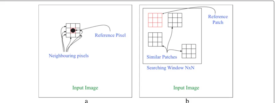
image filtering. A pixel-based image filtering scheme is mainly a proximity operation used for manipulating one pixel at a time (pixel-wise) based on its spatial neighbor-ing pixels located within a kernel. On the other hand, in patch-based image filtering, the noisy image is divided into patches, or “blocks,” which are then manipulated separately in order to provide an estimate of the true pixel values (patch-wise) based on similar patches located within a search window. This approach utilizes the redun-dancy and the similarity among the various parts of the input image. Figure 1 shows the mechanism of the two approaches.
Fig. 1Image denoising approaches:afiltering based on neighboring pixels located within a kernel in pixel-based denoising schemes andbfiltering based on patches located within a search window in patch-based denoising schemes
It is now common in image denoising field to uti-lize patch-based models and algorithms instead of pixel-based approaches to produce most promising estimate of the noise-free images. However, there are both advan-tages and disadvanadvan-tages in the use of patch-based models and algorithms. There are several advantages of patch-based approaches. Smoothing flat regions is the most important aspect. Redundancy between patches enable patch-based approaches to properly smooth flat reigns. A second advantage of using patch-based models and algo-rithms approaches is that it can preserve fine image details and sharp edges. However, there could be some disad-vantages for patch-based models and algorithms. First, although similarity between patches assists in estimating flat regions, so is the averaging. It is, therefore, quite time-consuming to group and compare similar patches. This might mean that each patch has multiple estimates and patches are overlapped. Secondly, while it may be that patterns and textures seem clear with less noise, patch-based models and algorithms usually exploit large number of parameters, which can be extremely difficult to adjust properly. We believe that the advantages of patch-based methods far outweigh their disadvantages, as modern computers are significantly fast, and have large memory spaces.
In this work, the patch-based image denoising schemes are analyzed from two different aspects: (1) the perfor-mance of patch-based denoising techniques in terms of image denoising quality and (2) the performance of patch-based denoising techniques in terms of computational time, where various patch-based denoising techniques are addressed.
A literature survey was conducted to evaluate the most recent patch-based denoising improvements for additive
noise. Following the literature survey, there is an empirical study, which is used to evaluate the performance of var-ious patch-based denoising techniques in terms of their accuracy and run times at various noise levels.
2 Patch-based image filtering
In patch-based denoising techniques, the input noisy image is divided into patches (i.e., blocks). The blocks are then manipulated separately in order to provide an estimate of the true pixel values. In this section, various patch-based image denoising algorithms are presented and their efficiency with respect to image denoising are studied.
2.1 Averaging patch-based: non-local means
Fig. 2Similarity between patches.aNL-Means patches as a raster scan in a search window.bPatch P3 is similar to P1 more than patch P2; hence, P3 will get a weight larger than P2 weight
P1 and P3, should be assigned a larger weight than that to be assigned to P2. The edges in NL-Means filtering are preserved regardless of their direction.
The estimated value NL-Means[v]i, for a pixeli, is
com-puted as:
NL-Means[v]i=
j∈I
ω(i,j)[v]j, (1)
where [v]i and [v]j are pixel intensities at locationsiand j, respectively, andω(i,j)is a similarity measure between the pixelsiandj. The similarity measure weight satisfies the condition 0 ≤ ω(i,j) ≤ 1 and jω(j,i) = 1. The similarity weight depends on the gray level similarity and the Euclidean distance between vectorsN[v]i andN[v]j,
whereN[v]k denotes a square neighborhood of fixed size
and centered at a pixelk. The weights are described as:
ω(i,j)= 1 Z(i)e
−(N[v]i)−(N[v]j)2
h2 , (2)
where Z(i) is a normalization factor and his a filtering parameter set depending on the noise level.
The level of noise determines the sizes needed for the search window and patches. For a robust comparison between patches, the size of the patches increases when the noise level is high. Accordingly, the value of the fil-tering parameter hincreases as the size of the patch is increased. Meanwhile, the size of the search window must be increased in order to find more similar patches.
NL-Means filter is considered the cornerstone of many patch-based denoising methods. It can be adapted eas-ily to many other applications, such as, multi-view image denoising. Nevertheless, there are some disadvantages of NL-Means filter. The filter is computationally expensive
due to the large amount of weight computations between similar patches. Another disadvantage is that the NL-Means filter is a spatial domain filter though convolution can be easily implemented in the frequency domain.
NL-Means filter has too many modifications. Improving the way of assigning the weights between patches would improve the performance of the NL-Means method. Hed-jam et al. [25] improved the process of adjusting the weights in the NL-Means by using Markovian clustering. Wu et al. [63] used a statistical shrinkage perspective when assigning the weights in NL-Means via using James-Stein [30] shrinkage estimator. Lai and Dou [35] introduced an improved neighborhood pre-classification strategy for optimized weight kernels of NL-Means filter. Khan and El-Sakka [32] introduced a variant of the NL-Means scheme by using a thresholding step to reduce the number of similar patches before weight averaging the patches.
NL-Means filter could be adapted to improve other image processing applications (e.g., segmentation, recog-nition, and video denoising). Zhan et al. [66] introduced an extension to the NL-Means method for ultrasonic speckle reduction. They assigned the patch similar-ity weights iteratively in a lower dimensional subspace using principal component analysis (PCA). Xu et al. [65] adapted the NL-Means to be use for microscopy cell images via a frequency transform. Genin et al. [20] adapted a modified version of the NL-Means filter for detecting small objects by background suppression. Background pixels are estimated by a weighted average depending on the similarity between neighborhoods pix-els. Kim et al. [33] adapted the NL-Means filter for noise reduction and enhancement of extremely low-light video. They use a motion adaptive temporal filter using gamma correction with adaptive thresholds before the NL-Means filter. Xu et al. [64] adapted the idea of patching from the NL-Means for filtering polarimetric synthetic aperture radar (POL-SAR) images; they use simultaneous sparse coding for transferring the patches into the frequency domain before assigning the weights.
2.2 Probabilistic patch-based filter
The probabilistic patch-based (PPB) filter, which works in the spatial domain, was proposed by Deledalle et al. [12] as an extension of the NL-Means filter. The PPB approach is one of a few denoising techniques that can provide a general denoising methodology for various noise mod-els. Thus, it is more general than the NL-Means and can be applied where there is additive noise or multiplicative speckle noise. The PPB filter is a statistically based similar-ity scheme that depends on the distribution model of the noise. The weighted average is used for the Gaussian noise distribution in the NL-Means, but the PPB filter applies smoothing based on the maximum likelihood estimator (MLE). The PPB is expressed as a weighted maximum likelihood estimation (WMLE) problem. The weight is derived from the data by improving the isotropy of the filter—non-iterative probabilistic patch-based filter (Non-iPPB)—and it can be iteratively defined based on the sim-ilarity of the patches—iterative probabilistic patch-based filter (It-PPB).
2.2.1 Weighted maximum likelihood estimator
Using a weighted maximum likelihood estimation for image denoising is not a new technique; it was first used for image denoising by Polzehl and Spokoiny [51, 52]. PPB redefined the weights in term of a patch-based approach. PPB image denoising is considered to be an estimationuˆ
of the true imageuwhich originates from the noisy image υ. The images are defined over a discrete regular grid. A pixel value is described asi, and its neighbor isjat the location(x,y)∈. The noise model is considered as being
defined by the parametric noise distribution “likelihood”
p(i|θi∗), whereθi∗is an unknown space-varying parame-ter. The denoising of an image is equivalent to finding the best estimationθˆi forθi∗for all pixels. The MLE at each
location(x,y)estimatesθˆifrom a setSθ∗
i of the distributed
random variables around it by:
ˆ
θi = arg max
θi
j∈Sθ∗ i
logpj|θi
, (3)
= arg max
θi
j δSθ∗
i(j)logp
j|θi
,
whereδSθ∗
i is an indicator function forSθ ∗
i (i.e.,δSθi∗ =1 if j ∈ Sθ∗
i or 0 otherwise). The indicator function has been
derived from the data as weightsω(i,j) ≥ 0 in Polzehl and Spokoiny [52] and Polzehl and Tabelow [51], where it is used as weight for adaptive pixel-wise filters. However, the indicator function in PPB is used as weight function to form the WMLE:
ˆ
θi=arg max
θi
j
ω(i,j)logp(j|θi). (4)
2.2.2 Defining the weight between patches
In Subsection 2.1, the weights in the non-local means fil-ter are defined by comparing the similarities of the two patches [v]iand [v]jcentered around the two locationsi
andj, respectively. A weighted Euclidian distance between the two patches defines the level of similarity. The objec-tive of the PPB filter is to generalize and extend the idea of the Euclidean distance weight used in the non-local means filter so that it can be adapted to non-additive noise models. The weights used in the probabilistic patch-based method are estimated using the probability of the two patches in a noisy image having the same parameters. By following the same idea as the weight in the non-local means filter and assuming equal values foriandjin the two statically similar patches [v]i and [v]j, PPB weights
would be defined as:
ω(i,j)(PPB)=p
θ[∗v]i=θ ∗ [v]j |υ
1/h
, (5)
where θ[∗v]
i and θ ∗
[v]j are the patches extracted from the
imageθ∗andhis larger than 0 , which indicates the size
of the patch in PPB. The h acts as σ in the NL-Means
algorithm in order to control the filtering amount. The probability of the similarity of the patches pixels is decom-posed into a product of the probabilities ofk neighbors:
kp
θ∗
i,k =θj∗,k |υi,k,υj,k
.
2.2.3 Iterative WMLE denoising
product of two terms: (1) the probability of the similar-ity between the noisy patches as described in Subsection 2.2.2 and (2) the probability of the similarity derived from the previous iteration.
Assume that the previous estimation at t iteration is
ˆ
θt−1forθ∗. Then, the formula in Eq. 5 can be expressed as:
ω(i,j)(It−PPB)=pθ[∗v] i=θ
∗ [v]j |υ,θˆ
t−11h
. (6)
This is similar to what was achieved in Subsection 2.2.2, where the probability of the similarity is decomposed into a product of the probabilities of the k neighbors:
kp
θ∗
i,k=θj∗,k|υi,k,υj,k,θˆt−1
.
From the Bayesian framework, the naïve Bayes model can be fitted with the maximum likelihood concept. The probability is estimated using the prior probability and can be presumed to be proportional to the likelihood:
pυi,k,υj,k,θˆt−1|θi∗,k=θj∗,k. (7)
The similarity likelihood is computed using:
pθi∗,k =θj∗,k |υi,k,υj,k,θˆt−1
∝ p
υi,k,υj,k |θi∗,k =θj∗,k
likelihood
×p
θi∗,k=θj∗,k| ˆθt−1
prior
. (8)
The likelihood term is to compute the degree of similar-ity between the patches, and the prior term is to compare the two probability distributions from the previous itera-tion, similar to Polzehl and Spokoiny [51].
The scheme, Fig. 3, shows the procedure of iteratively competing the weights in the PPB algorithm. The proce-dure for defining the weights is estimated iteratively by (1) the PPB weights estimator (PPBWE) uses the like-lihood term and the estimated value from the previous iteration in order to compute the prior term (Eq. 8), (2) WMLE uses the PPBWE estimation and the noisy image in order to estimate the new weight (Eq. 4), and (3) the
PPBWE and the WMLE steps are repeated until there is no difference in the estimations made from the two steps.
2.2.4 Algorithm used in the case of Gaussian noise
The PPB filter can be used for filtering additive white Gaussian noise (AWGN). By assuming the AWGN model, the values of the pixelsI of the patch [v]iare distributed
based on the Gaussian distributionℵu,σ2. Here,u is
the noiseless image andσ the noise variance. The noise-less imageucan be estimated by the weighted average that maximizes the WMLE defined in Eq. 4:
¨
ui(WMLE)=
jω
i,jIj2
jω
i,j . (9)
In order to estimate the weighted averageωi,j, two terms are considered: the likelihood and the prior terms. The likelihood function is discretized as:
pIi,k,Ij,k| ¨ui,k = ¨uj,k
likelihood
∝exp
−|Ii−Ij|2
4σ2
, (10)
and the prior term is discretized as:
pu¨i,k = ¨uj,k | ¨ut−1 prior ∝exp −1 T
| ¨uti−1,k − ¨utj,−1k |2
σ2
.
(11)
By combining the two terms in Eqs. 10 and 11, the weight at any iteration is defined as:
ω(i,j)(It−PPB)=
exp − n 1 h
|Ii−Ij|2 4σ2 +T1
|¨uti−,k1−¨utj−,k1|2
σ2
,
(12)
wherenis number of pixels andTis a constant similar to
hin Eq. 2. When there is no iteration “posterior term = 0,” the filter performs similar to the NL-Means filter.
PPB filter has several advantages and disadvantages. The main advantage of PPB filtering is that it is a statistical-based approach, which can be utilized for suppressing additive Gaussian noise and/or multiplicative speckle noise. Also, this filter can be adjusted as an iterative fil-ter or not. Nevertheless, the main drawback of this filfil-ter is the suppression of fine and dark details when denoising. Another disadvantage of the filter is the high computa-tional cost when used as an iterative filter.
A further extend patch log likelihood (EPLL) filter, similar to probabilistic patch-based filter, was proposed recently by Papyan and Elad [47] via considering a multi-scale prior.
2.3 Dictionary learning
Dictionary learning (DL) is utilized as a replacement for the use of a fixed dictionary for representing data. From the 1970s, data can be represented by using a fixed dictio-nary, for instance, Fourier of Boussinesq [5] and Wavelets of Haar [23]. In 1996, Olshausen and Field [45] proposed an approach to learn the dictionary from a data in order to optimize the sparsity of the data. The dictionary learn-ing or k-means slearn-ingular value decomposition (K-SVD) was first adapted to image denoising in 2006 by Aharon et al. [1]. Dictionary learning method finds the best dic-tionaryD = (di)zi=1ofzatomsdi ∈ Rnthat sparses the setY = yjmj=1 ∈ Rn×mof signalsyj ∈ Rm. In order to filter a noisy image, each signalyjis considered as a patch extracted from the noisy image. The sparse code of signal datay = yjforj = 1,. . .,nis obtained by minimizing a constrained optimization0:
min
x0≤k
= 1
2y−Dx
2
, (13)
where k > 0 controls the amount of sparsity, and 0 pseudo-norm is defined by:
xo= {i:xi=0}. (14)
In dictionary learning, optimization is performed on the dictionaryDand the coefficientsX=xj
m
j=1∈Rp×mfor j= 1,. . .,n, where the set of coefficients isxjof the data yj. The joint optimization is written as:
arg min
D∈ ,X∈χk
E(X,D)= 1
2Y−DX
2= 1
2
m
j=1
yj−Dxj2,
(15)
where is the constraint set:
=D∈Rn×p:∀i D.,i ≤1. (16) The sparsity constraint is set onχk , which is the unit
normalization of the dictionary columns: χk =
X∈Rp×m:∀i X.,i0≤k. (17)
Peyré and Fadili [49] proposed using a block-coordinate descent minimization approach used by Tseng [59] in order to minimizeXandD.
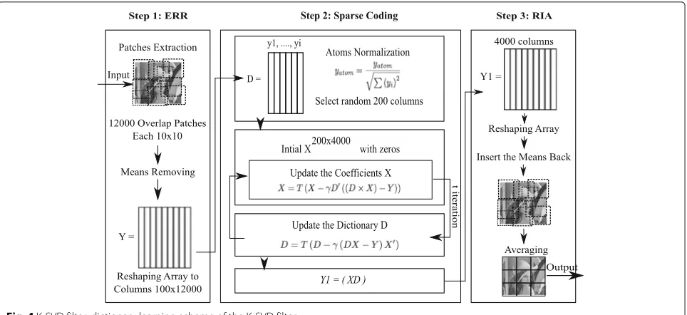
The dictionary learning algorithm depends mainly on three steps: (1) patch extraction, (2) sparse coding, and (3) patch construction. In the first step, several patches are randomly extracted from the whole input image. In the sparse coding step, the energies of theXandD dic-tionaries are iteratively minimized. Patch averaging and reconstruction occurs in the patch reconstruction step. Each of the three steps has stages:
1. Patch extraction step:
• The mean of each patch is removed from each
pixels value.
• Patches are sorted based on their energy, those
with a high level of energy are kept by thresholding.
• Patches are reshaped as columns in order to
formY.
2. Sparse coding step:
• Each atom in the columns is normalized in
order to form the initial dictionaryD.
• Number of the columns is reduced again, before
computing theX coefficients.
• TheX dictionary is initially started with zeros.
• The coefficients of dictionaryX is updated by:
X=TX−γD((D−X)−Y),
whereT is the thresholding.
• The dictionaryD is updated again by:
D=TD−γ(DX−X)−X.
• K is the number of iterations, which is used to
minimize theX and D dictionaries by updating
them iteratively.
• Finally, the coefficients of dictionaryX are
multiplied by dictionaryD.
3. Patch construction step:
• The result of the multiplication is a new array,
Y1.
• The columns ofY1are reshaped to form
patches.
• Re-inserting the averages to the patches comes
before averaging the patches to replace the noisy patch.
The scheme in Fig. 4 shows the steps of the dictionary learning method for denoising images.
Fig. 4K-SVD filter: dictionary learning scheme of the K-SVD filter
of the DL is the low number of parameters when com-pared to other patch-based denoising methods. However, DL has some drawbacks. The main disadvantage of DL is the computational burden due to several iterations for computing the singular value decomposition. Moreover, DL does not handle images with many flat patches very well because the singular value decomposition is more sensitive to textured patches.
The DL method has many modifications. Tian and Wang [57] made DL more sparsely representative in the case of less observation values by proposing an adap-tive orthogonal matching pursuit to adapadap-tively ensure the sample size. Some of the modifications aim to adapt the idea of denoising based on dictionary learning to other image processing applications. Chen et al. [10] general-ized the idea of the learning dictionary to explore identity information in multiple frames of videos. They gener-ated a sparse representation from multiple video frames for face and body part recognitions. Fu et al. [19] pro-posed an effective model based on DL for hyperspectral image (HSI) denoising by considering sparsity across the spatial-spectral domain, high correlation across spectra, and non-local self-similarity over space. Kang et al. [31] proposed a feature-based approach for assessing sim-ilarity between images. After extracting feature points from an image, they utilize dictionary learning. Then, they measured the similarity between images in terms of sparse representation. A novel self-learning based image decomposition framework was presented by Huang et al. [27]. Their framework performs unsupervised cluster-ing on the observed dictionary via affinity propagation that allows effectively to identify images components with similar context information. The framework can
automatically determine the undesirable random noisy components from true image components directly from a noisy image. Dictionary learning algorithm was adapted to filter Chinese character images by Shi et al. [54]. They divided the image frequency to low and high frequen-cies. While a Butterworth low-pass filter was utilized to filter low frequency, the K-SVD dictionary learning algo-rithm was proposed to filter high-frequency parts which consists of structure of Chinese characters.
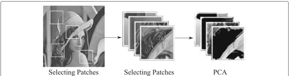
2.4 Patch-based PCA
Recently, over-complete dictionaries with sparse repre-sentation techniques became very widespread in image denoising [1, 40, 41], and they are one of the state-of-the-art denoising algorithms. These methods use over-complete dictionaries derived from enormous image sets or from the noisy image itself. They outperform other denoising techniques due to their ability to provide an appropriate basis for separating noisy signals from the true image signals, so they suppress more noise and preserve edges. Despite the fact that over-complete dic-tionaries are frequently used for image denoising, such dictionaries are sophisticated and quite expensive in terms of memory usage and time. However, patch-based princi-pal component analysis (PB-PCA) of Deledalle et al. [13] is a modification of the dictionary methods.
component analysis. The next step is to threshold the patches’ coefficients in the dictionaries. This idea is simi-lar to the wavelet denoising methods used in [8, 9, 14], in which they use either hard thresholding or soft threshold-ing for zerothreshold-ing the coefficients. Figure 5 shows extractthreshold-ing patches used in the PB-PCA method from an image and grouping them before computing the PCA.
For the problem of denoising an image that is inter-rupted by AWGN, the patch model has the following formula:
[v]i=[u]i+zi,i=1, ..,n−1, (18)
where [u]iis the true image patch,ziis the AWGN noise,
[v]iis the noisy patch, andnis the number of patches. By
assuming [v]i, .., [v]i−1are a group of overlapped patches
of size N × N extracted from the noisy image υ, the
covariance matrix is the sum of:
= 1
n n
i=1
[v]i[v]i− ¯υυ¯, (19)
where
¯
υ= 1 n
n
i=1
[v]i.
In PCA, the singular value decomposition (SVD) of
the covariance matrix is processed. Moreover, the
eigenvaluesg1,· · ·,gn−1of the covariance matrix and the corresponding eigenvectorsG1,· · ·,Gn−1are calculated. Eigenvectors are called the principal components “axis” of the processed data and are used to form an orthogonal basis,Giis the theith principal axis of the data. Due to the
orthogonal basis of the principal components, an image patch can be decomposed as [v]i= ni=1[v]i|GiGi.
Figure 6b, c shows the first and last 16 principal axes of the all patches obtained from the house image shown in Fig. 6a.
By assuming that the true image pixels have a low-dimensional subspace and the noise is spread in all direc-tions, projecting the axes into the first axis would suppress the noise in the noisy image. Projecting the axes is called
coefficient thresholding, and it is done by using an appro-priate shrinkage function. A general formula for estimat-ing a true image is:
ˆ
[u]i= ¯υ+ n
i=1
η ([v]i− ¯υ |Gi)Gi, (20)
whereηis the shrinkage function.
PB-PCA filtering method has been tested with four shrinkage functions: (1) soft thresholding (ST); (2) hard thresholding (HT); (3) Keep or Kill (KoK), and (4) Wiener filter [62]. Figure 7 shows a comparison between the four different projection methods into the basis by PCA for the
House andCameramanimages. From Fig. 7, it can be seen that hard thresholding with a large number of axes is the best of the four projection methods. Using a Wiener filter as a shrinkage function for the PCA has been pro-posed by Muresan and Parks [44, 67]. The Zhang et al. [67] algorithm will be discussed in Subsections 2.4.1.
PB-PCA has three variants based on how each set of patches is collected from the input noisy image before the PCA process. In PB-PCA, the three variants for collect-ing patches are globally, locally, or hierarchically. Figure 8 shows the best means of collecting the patch sets globally, locally, or hierarchically. These variants are discussed in the following subsections.
2.4.1 Patch-based global PCA
Collecting patches for a PCA can be done globally from the entire noisy image in patch-based global PCA (PGPCA). This approach is faster than the other approaches, which need time to divide the image into sub-images before computing the PCA coefficients. However, it has less filtering quality. Collecting patches globally for PCA filtering has been used in Bacchelli and Papi [2] and Zhang et al. [67]. The Bacchelli and Papi algorithm uses a linear transformation, “a wavelet transform,” before com-puting the PCA in order to achieve better results. The Zhang et al. algorithm collects patches globally, but it computes the PCA in two stages.
Fig. 6The principal components “axis” of the house image:ais the input image,bis the first 16 principal axes of the all patches obtained from the house image, andcis the last 16 principal axes of the all patches obtained from the house image [13]
The PGPCA approaches cannot compete with other local or semi-local approaches, which consider the high level of redundancy occurring between neighboring patches. In the global PGPCA, one original basis for the whole image, which impacts negatively on the denoising process. The global PGPCA does not identify the rare patches because they do not exert a strong influence on the total variance. However, an allowance can be made for these limitations by considering the local redundancy between patches.
2.4.2 Patch-based local PCA
In the patch-based local PCA (PLPCA) approach, patches are collected locally in order to overcome the limitations of the global PGPCA approach. The local collection of patches means that the patches are collected within a small region of interest in the noisy image. A fixed search windowN ×N is applied to the whole image. Since the patches are overlapped in PLPCA, there will be multiple estimates for a single pixel. Averaging is used to compute a single pixel’s value.
The advantage of this approach is that the orthonor-mal basis is adapted only to the sub-image and not to the whole image. However, this approach has two limitations: the overfitting and the fact that it is time-consuming. The overfitting problem is due to the limited number of patches on which to compute the PCA. PLPCA is extremely time-consuming because the PCA needs to be computed repeatedly.
Fei et al. [18] collected patches locally, but they improved their approach by using geometric structure clustering to guarantee that only patches with similar properties were gathered. Pal et al. [46] considered patch redundancy in order to improve on the global two-stage PCA approach of Zhang et al. A sliding window that
moves with a step s = Wp−1
2 , where s is the step size
andWpis the window’s current location was utilized as a
modification in order to reduce the time-consuming ele-ment of the PLPCA approach. The computational time is divided bys2without losing the denoising quality. Zhang et al. [68] proposed using similar patch-based local PCA
Fig. 8Collecting a set of patches in PB-PCA filtering:aglobal PCA,blocal PCA, andchierarchical PCA
filter with an extended step where a Wiener filter is finally applied.
2.4.3 Patch-based hierarchical PCA
In the patch-based hierarchical PCA (PHPCA) approach, an algorithm builds a hierarchy cluster of the patches. Clustering is the task of grouping a set of patches into the same cluster, i.e., set. There are different cluster models; each model has several clustering algorithms. The models include connectivity models (e.g., hierarchical cluster-ing) and centroid models (e.g., k-means). The hierarchi-cal clustering is based on the concept of the grouping of patches according to a maximum distance between patches. Patches are represented as a dendogram, which is a Greek word meaning a tree diagram that illustrates the arrangement of the patches. In centroid models, vectors are assigned usually to a numberkof fixed clusters. For more information about the clustering models, readers are referred to Chapter 17 inIntroduction to Information Retrievalby Manning et al. [42].
The objective of the PHPCA approach is to offer a solu-tion that can provide a result between the PGPCA and PLPCA approaches, which is less time-consuming than the local approaches and is more adapted to local sub-images. PHPCA uses a geometric partitioning to first divide the image into four areas, and then it estimates the
principal axis for each area. Each area has its own prin-cipal components. This process is repeated until the end of the tree is reached. Several dictionaries share the first axes. Figure 8c shows how an image can be divided to sub-images.
The most important advantage of patch-based PCA fil-ter is its ability to produce a solution for image denoising using a modest orthogonal dictionary with PCA of the input data. Moreover, a patch-based PCA filter provides various grouping stages to fit user needs—local, global, or hierarchical. The main disadvantage of PB-PCA is its susceptibility to overfitting due to few training patches when performing the PCA locally. Also, PB-PCA is quite expensive in terms of time since PCA needs to be per-formed repeatedly.
2.5 Sparse 3D transform-domain collaborative filtering Block matching 3D algorithm (BM3D) is the state-of-the-art denoising technique by Dabov et al. [11]. It is based on modified sparse representation in the frequency domain. BM3D groups the patches into 3D data arrays instead of into 2D arrays, then it applies a modified sparse repre-sentation in the frequency domain. Collaborative filtering is used to deal with the 3D arrays. BM3D’s algorithm depends on two steps: (1) collaborative hard thresholding and (2) the collaborative Wiener filtering. The two steps
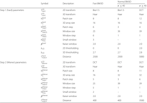
Table 1Parameters set for the original BM3D
Symbol Description Fast BM3D Normal BM3D
σ ≤40 σ ≥40
Step 1 (hard) parameters T2D
hard 2D transform Bior1.5 Bior1.5 DCT
T3D
hard 3D transform Haar Haar Haar
Nhard
1 Patch size 8 8 12
Nhard
2 3D array size 16 16 16
Nhard
step1 Patch step 6 3 4
Nhard
search Window size 25 39 39
Nhardstep2 Window step 6 1 1
NhardPrev. Small window 3 – –
βhard Kaiser window 2.0 2.0 2.0
λ2D 2D thresholding 0 0 2.0
λ3D 3D thresholding 2.7 2.7 2.8
Tmatchhard Distance 2500 2500 5000
Step 2 (Wiener) parameters TWiener2D 2D transform DCT DCT DCT
TWiener3D 3D transform Haar Haar Haar
NWiener1 Patch size 8 8 11
NWiener2 3D array size 16 32 32
NWienerstep1 Patch step 5 3 6
NWienersearch Window size 25 39 39
NWiener
step2 Window step 5 1 1
NWiener
Prev. Small window 2 – –
βWiener Kaiser window 2.0 2.0 2.0
TWiener
match Distance 400 400 3500
allow the BM3D to suppress more noise and to preserve more detail. The amount of noise is suppressed in the thresholding step, and the details are restored in the sec-ond step. Collaborative hard thresholding has three func-tions: (1) 3D transform, (2) shrinkage, and (3) 3D inverse transform. The patches in the 3D arrays are overlapped, so a weighted average is used to obtain one estimation for each pixel. Aggregation is the averaging procedure. A sig-nificant filter is obtained by using the BM3D algorithm. The scheme in Fig. 9 shows the two steps of BM3D fil-tering. Below, the two steps of the BM3D algorithm are described. First, the collaborative hard thresholding step is explained. Then, using the collaborative Wiener filtering is discussed.
2.5.1 Step 1: thresholding
Grouping: Similar to the NL-Means, a search window is used to determine the similarity between the patches. The search window is used in order to benefit from the high redundancy among the neighboring patches. There are several different grouping techniques. A number of these techniques have been discussed in this survey. Some other useful techniques for grouping could be considered for
patch grouping, such as vector quantization [21],k-means clustering [39], self-organizing maps [34], and others dis-cussed in this survey [29]. However, grouping in BM3D is based on the similarity distance between patches, the “Euclidian distance.” The grouping stage is the first of the two steps in which similar patches are gathered to form 3D arrays. Similarity is computed according to the dis-tances between the patches. Patches with a distance that is below a fixed threshold are considered to be similar and are grouped into the 3D array. Before measuring the distance, a coarse pre-filtering is used to linearly trans-form the patches using a 2D linear transtrans-formation such as multiple wavelet transforms [15, 53]. The formulation in Eq. 21 is used to compute the similarity distance between patches,
Dst[v]i, [v]j
= γ2D
T2D
hard([v]i)
−γ2DT2D hard([v]j)22
Nhard 1
2 ,
(21)
where [v]i, [v]jare respectively the reference patches ati
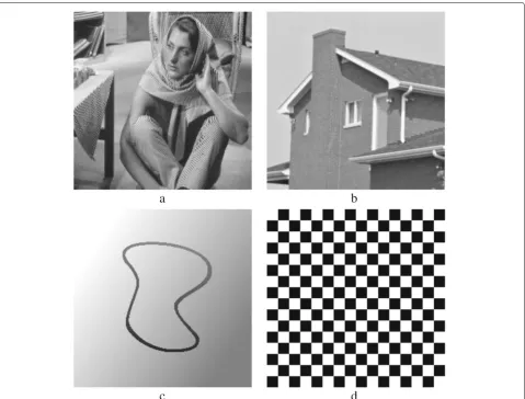
Fig. 10The four used images in the experiment:aBarbaraimage 512×512,bHouseimage 256×256,cCurvedBandimage 257×257, and
dChessboardimage 256×256
γ2D is a hard-thresholding operator equals toλ 2D ×σ,
andN1hard2is the patch sizeN×N.σ is the estimated noise standard deviation.γ2Dmakes all coefficients with
absolute value less than the threshold(λ2D×σ)equal to
zero, and it leaves the other coefficients unchanged. After computing the Euclidian distance, grouping the similar patches into a 3D array is required. The formulation in Eq. 22 is used for gathering similar patches.
3DSihard=j∈: Dst[v]i, [v]j
≤Tmatchhard , (22)
where 3DShardi is the constructed 3D array contains simi-lar patches andTmatchhard is the maximum distance between two similar patches. The maximum grouped patches size are restricted toN2hard. The next stage is to apply the col-laborative filter by (1) performing a 2D linear transform then a 1D linear transform, (2) shrinkage, and (3) inverting the 1D transform and the 2D linear transform.
Collaborative filtering: Once the 3D array is built, a col-laborative filter is used for suppressing the noise. A 3D transform is applied to the 3D array, before the shrinkage of the transforming coefficients. The 2D transformation in the grouping stage is applied along both horizontal and vertical lines for each patch, and then a third transfor-mation is conducted along the third diminution of the 3D array for the 3D transform. The formulation of the collaborative filter is:
3DuˆShard
i =T
3D−1
hard
γ3DT3D hard
3DShardi , (23)
Aggregation weights: At this stage, overlapped patches in the 3D array3DuˆShard
i
have multiple estimates for each pixel in the reference patch at the location i. A weighted averaging procedure is required to provide an estimate for each pixel. Weights in BM3D are inversely proportional to the total variance of the patches in the 3DuˆShard
i array. When the total variance is high, a small
weight is assigned to the patch.
The amount of the additive noise is independent when processing the collaborative filter in step 1 and step 2. Thus, the total variance is not the same after applying the collaborative filter in the first and second steps. In step 1, the total variance is computed byσ2×Nnon−zerohard , where
Nnon−zerohard is the number of non-zero coefficients after the hard thresholding. The total variance calculated in step 2 depends on the results of the Wiener filter coefficients, the weights of step 2 will be explained on the facing page. However, the weights for step 1 is equal to:
ωhard
i =
1
σ2×Nhard non−zero
,
1,
if→Nnon−zerohard ≥1
otherwise . (24)
2.5.2 Step two: Wiener filter coefficients
Grouping: Grouping in the second step is in some ways similar to the grouping in the first step; but here, the power spectrums of the first step are grouped, not just the patches from the noisy image. The same formula is used:
3DSWieneri = ⎧ ⎪ ⎪ ⎪ ⎨ ⎪ ⎪ ⎪ ⎩
j∈:
uˆShard
[v]i − ˆ uShard
[v]j 2
2
N1Wiener2 ≤T Wiener match ⎫ ⎪ ⎪ ⎪ ⎬ ⎪ ⎪ ⎪ ⎭ , (25)
whereuˆShard [v]i
anduˆShard [v]i
are the estimated sub-images from step 1 respectively at locationsiandj, respectively. At this stage there are two groups: (1) a group of similar patches derived from the noisy image and (2) a group of similar patches derived from the first step.
Collaborative filtering: After grouping the patches, a 3D transform is applied to the 3D array of the grouped patches. A Wiener shrinkage is applied to the transform coefficients of the 3D array. The definition of the Wiener shrinkage coefficients of the power spectrum of the first step is shown in the equation:
3DWSWiener
i =
T3DWiener3DSiWiener 2
T3DWiener3DSiWiener 2+σ2, (26)
whereT3DWiener is the 3D linear transform and 3DSiWiener
is the result of Eq. 25. The final stage in the collaborative
Wiener filtering of the second step is to multiply the Wiener shrinkage coefficients element-by-element by the 3D transform coefficients of the noisy image. The inverse of the 3D transform is applied. Multiplication and the inverse of the 3D transform are shown in the equation:
3DuˆSWiener
i =
T3DWiener−13DWSWiener
i ×
T3DWiener(3Dνi)
,
(27)
where 3Dνi is the 3D transform coefficients of the noisy
data.
Aggregation weights: Adjusting the weights in this step is not like the first step, which depends on the number of non-zero coefficients reached after the hard thresholding.
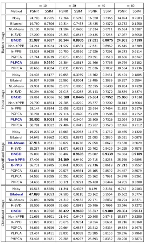
Table 2The performance of the denoising algorithms with various noise levels(σ )
The weights, here, depend on the Wiener shrinkage coef-ficients; the weights are assigned as:
ωWiener
i =σ−2WSWieneri −2
2 . (28)
The parameters set for the original BM3D is shown in Table 1; the table has some non-discussed parameters:
Nstep1hard: step size for searching the patches inside the search window
Nstep2hard: step size for moving the search window
NPrev.hard: small search window width for fast BM3D
βhard: the Kaiser window function one parameter for
reducing the borders effect Haar: a Haar transform
DCT: a discrete cosine transform Bior1.5: a biorthogonal wavelet
BM3D filter has advantages and disadvantages. The main advantage of BM3D filtering is that it yields great results with less loss of detail due to the smoothing and sharping stages. The BM3D filter is a fast method because it computes similarity between patches before the actual filtering procedure. Despite its many advan-tages, BM3D has several drawbacks. The performance of BM3D decreases with a high noise level(σ > 40), and it produces images with many artifacts. BM3D is more com-plex and less flexible to be adapted for domain-specific image processing applications. In addition, it is not easy to be parallelized. In addition, it has many parameters, and adjusting them optimally is a challenging task.
BM3D has two filtering steps and more than 20 eters. Improving the way of adjusting any of the 20 param-eters would participate on improving the output of the BM3D method. BM3D modifications would be catego-rized into four main categorizes: (1) modifications con-sider improving the shrinkage function, (2) modifications consider improving the transforms, (3) modifications con-sider improving the image similarity measures when col-lecting similar patches, and (4) modifications consider improving the Wiener filtering stages. Suwabe et al. [55] modified the way of collecting similar patches in the BM3D from non-locally to globally. They proposed using iterative filtering with Chebyshev polynomial approxima-tion (CPA) in order to collect the patches from the whole noisy image. Bashar and El-Sakka [3] replaced the fixed hard thresholding scheme with a learning-based adaptive hard thresholding scheme that considers the context of corresponding blocks. Hasan and El-Sakka [24] improved the Wiener filter of BM3D by maximizing the structural similarity (SSIM) [60] between patches instead of using the mean square error (MSE). Moreover, they introduced a 3D zigzag thresholding.
3 Results and discussions
In this section, various denoising methods are compared aiming to reduce additive white Gaussian noise (AWGN). The objective of this section is to experimentally study the performance of these methods, where the performance is
Table 3Execution time in seconds shows the speed of the denoising methods applied to the four images at various noise levels(σ )
Fig. 11Denoising methods performance: the performance of the denoising methods for the four images at various noise levels(σ )
0 0.2 0.4 0.6 0.8 1
Noisy AD Bilateral
NL−MeansK−SVDBM3DNon−itPPB
It−PPBPGPCAPLPCAPHPCA Barbara Image Results, σ = 10
SSIM
0 0.2 0.4 0.6 0.8 1
Noisy AD Bilateral
NL−MeansK− SVDBM3D
Non− itPP
B It−PP
B
PGPCAPLPCAPHPCA House Image Results, σ = 10
SSIM
0 0.2 0.4 0.6 0.8 1
Noisy AD Bilateral
NL−MeansK− SVDBM3D
Non
−itPPBIt−PPBPGPCAPLPCAPHPCA CurvedBand Image Results, σ = 10
SSIM
0 0.2 0.4 0.6 0.8 1
Noisy AD Bilateral
NL−
MeansK−SVDBM3D Non− itPP
B It−PP
B
PGPCAPLPCAPHPCA Chessboard Image Results, σ = 10
SSIM
0 0.2 0.4 0.6 0.8 1 Noisy AD Bilateral
NL−MeansK−SVDBM3DNon−itPPB
It−PPBPGPCAPLPCAPHPCA Barbara Image Results, σ = 20
SSIM 0 0.2 0.4 0.6 0.8 1 Noisy AD Bilateral NL−MeansK− SVDBM3D
Non− itPP
B It−PP
B
PGPCAPLPCAPHPCA House Image Results, σ = 20
SSIM 0 0.2 0.4 0.6 0.8 1 Noisy AD Bilateral NL−MeansK− SVDBM3D Non
−itPPBIt−PPBPGPCAPLPCAPHPCA CurvedBand Image Results, σ = 20
SSIM 0 0.2 0.4 0.6 0.8 1 Noisy AD Bilateral
NL−MeansK −SVDBM3D Non− itPP B It−PP B
PGPCAPLPCAPHPCA Chessboard Image Results, σ = 20
SSIM
Fig. 13The performance charts: four charts summarize the performance of the denoising methods for the four images when the noise is low (σ=20)
assessed at various noise levels. The issue of time con-sumption is also addressed. Four images are used to run this experiment. The images have been chosen carefully to help in distinguishing between the methods. The first two of the four images are natural scene images,Barbaraand
House; the other two are synthetic images,CurvedBand
andChessboard. TheChessboardimage is a binary image while the other three images are gray-scale images. The four images are shown in Fig. 10. The fine details inBarbaraimage helps in demonstrating how various methods preserve the image clarity, whereas the sharp
edges in the Houseimage helps in demonstrating how
various methods preserve edges. The gray gradations in
CurvedBandimage provide insight into the amount of smoothing that has been applied to images. The meth-ods are also tested with the binary pattern repetitions
in the Chessboard image. MatLab is used for this
experiment. The computer’s processor is an Intel (R) Core(TM) i7 CPU @ 3.40 GHz. In Subsections 3.1 and 3.2, the methods are evaluated both quantitatively and qualitatively.
3.1 Quantitative evaluation
In order to make an objective comparison between the results, two image similarity matrices are used: (1) the structural similarity and (2) the peak signal-to-noise ratio (PSNR). These quality metrics have been chosen for their capability to assess the level of the additive Gaussian noise degradation. The best result for SSIM is 1, while the PSNR has good result when its value is high. Equations 29 and 30 show the formulas for these two quality metrics, respectively:
SSIM(x,y)=
2μxμy+C1 2σxy+C2
μ2
x+μ2y+C1 σx2+σy2+C2
, (29)
wherexis the true reference image,yis the noisy image,
μx and μy are the mean of the true reference image
block and the noisy image block, respectively,σx andσy
0 5 10 15 20 25 30 35 40 45 AD Bilateral NL−Mean s BM3 D Non−itPPBIt−PPBPGPCAPLPCAPHPCA Speed Average
Barbara Image Results
Speed in Seconds
0 5 10 15 20 25 30 35 40 45 AD Bilateral NL−Means BM3 D Non−itPPB It−PP B PGPCAPLPCAPHPCA Speed Average House Image Results
Speed in Seconds
0 5 10 15 20 25 30 35 40 45 AD Bilateral NL−Means BM3 D Non−itPPBIt−PPBPGPCAPLPCAPHPCA Speed Average
CurvedBand Image Results
Speed in Seconds
0 5 10 15 20 25 30 35 40 45 AD Bilateral NL−Means BM3D Non−itPP B It−PP B PGPCAPLPCAPHPCA Speed Average
Chessboard Image Results
Speed in Seconds
Fig. 14The efficiency charts: four charts show the average of the consumed time in seconds for various denoising methods excluding K-SVD
andC2 are constants used to avoid instability. The peak
signal-to-noise ratio is defined as:
PSNR=10 log
(2n−1)2 MSE
, (30)
where MSE is the mean squared error andnis an integer number representing the number of bits per pixel. When
n=8, i.e., in case of gray-scale images, the PSNR formula is reduced to:
PSNR=10 log
2552 MSE
. (31)
A study conducted by Hore and Ziou [26] has revealed that SSIM is less sensitive to additive noise than PSNR.
They used F-score test to compare between SSIM and
PSNR which works for AWGN. Thus, the final conclusion in our study is driven based on SSIM.
The experimental results of the denoising methods are shown in Tables 2 and 3. The tables show the perfor-mance of the patch-based denoising methods along with
the famous pixel-based denoising methods: anisotropic diffusion (AD) by Perona and Malik [48] and the bilat-eral filter. In both tables, the methods are sorted from the oldest to the most recent.
The results in Table 2 are computed by measuring the differences between the original images and the denoised images. The default parameters shown in Table 1 were used for the BM3D method, these values are suggested by the authors of BM3D. The noise standard deviation of the noisy images, which methods depends heavily on it, is required to be adjusted accurately before the denoising process. In case the noise estimation was not given, Ghazi and Erdogan [22], Tai and Yang [56], and Liu et al. [37] offer more information about noise estimation. The highest values of SSIM and PSNR are highlighted with a bold font. Table 3 shows the execution time of the methods in seconds. The fastest patch-based methods are highlighted with a bold font.
Fig. 15DenoisedBarbaraimages:aOriginalBarbaraimage;bAWG noise,σ =40;cAD ;dbilateral filtering,eNL-Means filtering,fK-SVD,gBM3D, hnon-itPPB,iit-PPB,jPGPCA,kPLPCA, andlPHPCA
when denoising the Chessboard image at σ ≤ 10
because of the large number of flat regions. Using pixel-based methods is not recommended when standard deviation of a noisy image is above 40. Although promis-ing results have been achieved by BM3D when denoispromis-ing flat and textures scene images at high noise levelsσ >10, the performance of BM3D decreases when denoising
images have a lot of fine details regions at σ ≤ 10;
see the results of Barbara and House images in
Table 2.
Fig. 16Zoomed images of the denoisedBarbaraimage shown in Fig. 15:aoriginal Barbara’s pant;bAWG noise,σ=40;cAD (Perona & Malik); dbilateral filtering;eNL-Means filtering;fK-SVD;gBM3D;hNon-itPPB;iIt-PPB;jPGPCA;kPLPCA; andlPHPCA
after BM3D when they are used for natural scene images. The results of K-SVD and the iterative PPB are similar.
The two lines at the bottom of each chart presents the performance of pixel-wise methods: anisotropic dif-fusion and the bilateral filter. From the charts, we can conclude that the block-wise denoising methods perform better than the pixel-wise methods. When usingσ = 10
and σ = 20, the results are similar except with the
pixel-wise methods. The performance of the methods will be discussed in the following two paragraphs.
Bar charts are used in Fig. 12 to represent the
meth-ods performance when the noise level is low σ = 10.
Fig. 17Zoomed images of the denoisedBarbaraimage shown in Fig. 15:aoriginal Barbara’s eye cover fold;bAWG noise,σ =40;cAD (Perona & Malik);dbilateral filtering;eNL-Means filtering;fK-SVD;gBM3D;hNon-itPPB;iIt-PPB;jPGPCA;kPLPCA; andlPHPCA
denoising methods achieved better results when denois-ing the natural scene images. When the noise level is low
σ = 10, the top two denoising methods for denoising
the natural scene images are PHPCA and BM3D, whereas the top two denoising methods for denoising the synthetic images are BM3D and bilateral filter. Yet, the differences are insignificant.
The charts in Fig. 13 show the methods performance
when σ = 20. By increasing the noise level, the
con-trast between methods becomes obvious unlike when the
noise is lowσ = 10. BM3D achieved better results than other methods in all images. The patch-based denoising methods perform better than pixel-wise methods.
Fig. 18DenoisedHouseimages:aoriginalHouseimage;bAWG noise,σ=40;cAD (Perona & Malik);dbilateral filtering;eNL-Means filtering; fK-SVD;gBM3D;hNon-itPPB;iIt-PPB;jPGPCA;kPLPCA; andlPHPCA
the denoising step, it is the fastest patch-based method. The time consumed for various values of noise is almost the same, so the high level of noise does not greatly affect the time consumption of the various methods.
3.2 Qualitative evaluation
The evaluation in this subsection is a subjective eval-uation, where the quality of the denoised images is
addressed via the visual perception. Denoised images with AWGN(σ =40)are chosen to perform this evaluating. Figures 15, 18, 19, and 21 show the denoised images.
The results of denoising Barbara’s image are shown
Fig. 19DenoisedCurvedBandimages:aoriginalCurvedBandimage;bAWG noise,σ=40;cAD (Perona & Malik);dbilateral filtering;eNL-Means filtering;fK-SVD;gBM3D;hNon-itPPB;iIt-PPB;jPGPCA;kPLPCA; andlPHPCA
come after BM3D, Fig. 15f, j, k, l shows K-SVD and PCA patch-based results. They apply a good smoothing to the image, but some edges are destroyed. The non-local mean method applies less smoothing; thus, the textures shown in Fig. 15e inBarbara’s pants are preserved; a zoomed version of Fig. 15e is shown in Fig. 16e. Figure 15h, i shows how the PPB methods apply a good smoothing, but they fail to preserve sharp edges and textures, i.e.,Barbara’s
eye cover fold. Zoomed versions of Fig. 15h, i are shown in Fig. 17h, i.
Figure 18 shows the results of denoising the House
Fig. 20Zoomed images of the denoisedCurvedBandimage shown in Fig. 19:aoriginalCurvedBandimage;bAWG noise,σ=40cAD (Perona & Malik);dbilateral filtering;eNL-Means filtering;fK-SVD;gBM3D;hNon-itPPB;iIt-PPB;jPGPCA;kPLPCA; andlPHPCA
The edges are preserved when using K-SVD, but K-SVD fails to smooth properly flat areas, i.e., the sky in the
House image. Thin edges are not preserved with PCA patch-based methods.
Figure 19 shows the denoisedCurvedBandimage. PPB
methods and BM3D have the best results, the results are shown in Fig. 19g– i. Unlike BM3D, PPB methods succeed more in smoothing the gray gradations; zoomed versions
of Fig. 19g–i are shown in Fig. 20g–i. K-SVD and PCA patch-based methods have similar results, Fig. 19f, j, k, l shows these results. They preserve parts of the curve, but they do not smooth properly flat areas; zoomed versions of Fig. 19f, j, k, l are shown in Fig. 20f, j, k, l.
Figure 21 shows the denoised Chessboard image.
Fig. 21DenoisedChessboardimages:aoriginalChessboardimage;bAWG noise,σ=40;cAD (Perona & Malik);dbilateral filtering;eNL-Means filtering;fK-SVD;gBM3D;hNon-itPPB;iIt-PPB;jPGPCA;kPLPCA; andlPHPCA
NL-Means method has the second good result, unlike its performance on the other images. Figure 21e shows the result of NL-Means method. With the K-SVD method shown in Fig. 21f, edges are preserved and the flat areas are smoothed appropriately. Disappointed results are achieved by using PCA patch-based methods; Fig. 21j, k, l shows the result of using PCA patch-based methods.
4 Summary of contribution
the patch-based denoising techniques are also presented. Moreover, the review covers the issue of time. Finally, based on years of experience, we believe that this review will be helpful for researchers to choose suitable denoising techniques to be adapted further for their image process-ing applications.
5 Future research directions
Like any other image denoising approaches, many impor-tant research directions should remain in patch-based image denoising. Improving patch similarity measures is suggested for grouping accurately similar patches. More-over, the research should also produce tools with bet-ter shrinkage functions to suppress noise and preserve fine details. Finally, developing effective image transform strategies that meet the needs to differentiate between a true and noisy signal is strongly recommended.
6 Conclusions
Among the best denoising methods is patch-based denoising method, which includes BM3D, NL-Means, and K-SVD. This paper has dealt with the efficiency of each of these methods when compared to other patch-based denoising methods. Experimentally, BM3D method gives the best result; it performs very well on all images and at all levels of noise. K-SVD and PCA methods come second to BM3D. Although the sparsity is learned from the data itself in K-SVD, K-SVD fails to compete with BM3D. NL-Means gives an encouraging result at low levels of noise. Furthermore, PPB methods preserve the fine details but fails to do so with respect to the sharp edges.
K-SVD is incomparable with the other compared meth-ods in terms of its time consumption. As it is very expen-sive. In contrast, BM3D execution time is the best among the patch-based denoising methods because it computes all similarity between whole patches first before starting the actual denoising process.
Abbreviations
AD: Anisotropic diffusion; AWGN: Additive white Gaussian noise; BM3D: Block matching 3D algorithm; CPA: Chebyshev polynomial approximation; DL: Dictionary learning; EPLL: Extend patch log likelihood; HSI: Hyperspectral image; HT: Hard thresholding; It-PPB: Iterative probabilistic patch-based; K-SVD: K-means singular value decomposition; KoK: Keep or Kill; MLE: Maximum likelihood estimator; MSE: Mean square error; MSSIM: Mean structural similarity; NL-Means: Non-local means; NSERC: Natural sciences and engineering research council of Canada; Non-iPPB: Non-iterative probabilistic patch-based; PB-PCA: Patch-based principal component analysis; PCA: Principal components analysis; PGPCA: Patch-based global PCA; PHPCA: Patch-based hierarchical PCA; PLPCA: Patch-based local PCA; POL-SAR: Polarimetric synthetic aperture radar; PPB: Probabilistic patch-based; PPBWE: PPB weights Estimator; PSNR: Peak signal-to-noise ratio; SNR: Signal-to-noise ratio; SSIM: Structural similarity; ST: Soft thresholding; SVD: Singular value decomposition; WMLE: Weighted maximum likelihood estimation; XNL-Means: X-ray non-local means
Acknowledgements
This research is partially funded by the Natural Sciences and Engineering Research Council of Canada (NSERC). This research is also partially funded by Jeddah University, Jeddah, Saudi Arabia. These supports are greatly appreciated.
Funding
This research is partially funded by the Natural Sciences and Engineering Research Council of Canada (NSERC). This research is also partially funded by Jeddah University, Jeddah, Saudi Arabia.
Authors’ contributions
MES suggested the idea; MHA carried out the experiments. MES continuously supervised the experiments and suggested modifications. MHA prepared the manuscript draft, and MES edited and proofread the manuscript. Both authors read and approved the final manuscript.
Competing interests
The authors declare that they have no competing interests.
Publisher’s Note
Springer Nature remains neutral with regard to jurisdictional claims in published maps and institutional affiliations.
Author details
1Department of Computer Science, University of Jeddah, Asfan Road, 285,
Dhahban 23881, Jeddah, Saudi Arabia.2Department of Computer Science, Middlesex College, Western University, 1151 Richmond Street, N6A 5B7, London, Ontario, Canada.
Received: 31 August 2016 Accepted: 26 July 2017
References
1. M Aharon, M Elad, A Bruckstein, K-svd: An algorithm for designing overcomplete dictionaries for sparse representation. IEEE Trans. Sig. Process.54(11), 4311–4322 (2006). doi:10.1109/TSP.2006.881199 2. S Bacchelli, S Papi, Image denoising using principal component analysis
in the wavelet domain. J. Comput. Appl. Math.189, 606–621 (2006). doi:10.1016/j.cam.2005.04.030. Proceedings of The 11th International Congress on Computational and Applied Mathematics
3. F Bashar, MR El-Sakka, inProceedings of the 11th Joint Conference on Computer Vision, Imaging and Computer Graphics Theory and Applications. BM3D image denoising using learning-based adaptive hard thresholding, vol. 3:VISAPP, (Rome, 2016), pp. 204–214
4. EP Bennett, L McMillan, inACM SIGGRAPH 2005 Papers, ACM, New York, NY, USA, SIGGRAPH ’05. Video enhancement using per-pixel virtual exposures, (2005), pp. 845–852. doi:10.1145/1186822.1073272. http://doi.org/10. 1145/1073204.1073272
5. J Boussinesq,Théorie analytique de la chaleur(Gauthier-Villars, Paris, 1903) 6. A Buades, B Coll, JM Morel, inComputer Vision and Pattern Recognition,
2005. CVPR 2005. IEEE Computer Society Conference on, vol 2. A non-local algorithm for image denoising, (2005), pp. 60–65. doi:10.1109/CVPR.2005.38 7. C Chan, R Fulton, DD Feng, S Meikle, inIEEE Nuclear Science Symposuim
Medical Imaging Conference. Median non-local means filtering for low SNR image denoising: application to pet with anatomical knowledge, (2010), pp. 3613–3618. doi:10.1109/NSSMIC.2010.5874485
8. S Chang, B Yu, M Vetterli, Adaptive wavelet thresholding for image denoising and compression. IEEE Trans. Image Process.9(9), 1532–1546 (2000a). doi:10.1109/83.862633
9. S Chang, B Yu, M Vetterli, Spatially adaptive wavelet thresholding with context modeling for image denoising. IEEE Trans. Image Process.9(9), 1522–1531 (2000b). doi:10.1109/83.862630
10. YC Chen, VM Patel, PJ Phillips, R Chellappa, Dictionary-based face and person recognition from unconstrained video. IEEE Access.3, 1783–1798 (2015). doi:10.1109/ACCESS.2015.2485400
11. K Dabov, A Foi, V Katkovnik, K Egiazarian, Image denoising by sparse 3-d transform-domain collaborative filtering. IEEE Trans. Image Process.16(8), 2080–2095 (2007). doi:10.1109/TIP.2007.901238
12. CA Deledalle, L Denis, F Tupin, Iterative weighted maximum likelihood denoising with probabilistic patch-based weights. IEEE Trans. Image Process.18(12), 2661–2672 (2009). doi:10.1109/TIP.2009.2029593 13. CA Deledalle, J Salmon, A Dalalyan, inProceedings of the British Machine

![Fig. 6 The principal components “axis” of the house image: a is the input image, b is the first 16 principal axes of the all patches obtained from thehouse image, and c is the last 16 principal axes of the all patches obtained from the house image [13]](https://thumb-us.123doks.com/thumbv2/123dok_us/892673.1586716/9.595.58.542.558.695/principal-components-principal-patches-obtained-thehouse-principal-obtained.webp)