Per-Sample Multiple Kernel Approach for Visual Concept Learning

Volume 2010, Article ID 461450,13pages doi:10.1155/2010/461450

Research Article

Per-Sample Multiple Kernel Approach for

Visual Concept Learning

Jingjing Yang,

_{Yuanning Li,}

_{Yonghong Tian,}

_{Ling-Yu Duan,}

_{and Wen Gao}

2_{National Engineering Laboratory for Video Technology, School of EE & CS, Peking University, Beijing 100871, China} 3_{Graduate University, Chinese Academy of Sciences, Beijing 100039, China}

Correspondence should be addressed to Yonghong Tian,[email protected]

Received 1 May 2009; Revised 22 November 2009; Accepted 19 January 2010

Academic Editor: Benoit Huet

Copyright © 2010 Jingjing Yang et al. This is an open access article distributed under the Creative Commons Attribution License, which permits unrestricted use, distribution, and reproduction in any medium, provided the original work is properly cited.

Learning visual concepts from images is an important yet challenging problem in computer vision and multimedia research areas. Multiple kernel learning (MKL) methods have shown great advantages in visual concept learning. As a visual concept often exhibits great appearance variance, a canonical MKL approach may not generate satisfactory results when a uniform kernel combination is applied over the input space. In this paper, we propose a per-sample multiple kernel learning (PS-MKL) approach to take into account intraclass diversity for improving discrimination. PS-MKL determines sample-wise kernel weights according to kernel functions and training samples. Kernel weights as well as kernel-based classifiers are jointly learned. For efficient learning, PS-MKL employs a sample selection strategy. Extensive experiments are carried out over three benchmarking datasets of different characteristics including Caltech101, WikipediaMM, and Pascal VOC’07. PS-MKL has achieved encouraging performance, comparable to the state of the art, which has outperformed a canonical MKL.

1. Introduction

Visual concept learning is an important topic in image and video indexing and retrieval. Advanced machine learning techniques have been widely employed to map low-level visual features to visual concepts, such as scenes (e.g., indoor/outdoor [1], natural scenes [2]) and objects (e.g., airplane/motorbike/face) [3,4]. Generally, a visual concept classifier is learnt from manually labeled images in a supervised manner and unseen images are categorized into one of the learnt concepts with a classifier. However, a well-trained concept classifier on a small dataset may not be expected to work fairly well on a much larger-scale image or video corpus due to the well-known semantic gap [5].

Learning visual concepts from numerous images is a challenging problem in real applications. For a concept, its image instances are often assumed to produce similarity in different attributes (e.g., scale, shape, color, and texture). As shown inFigure 1(a), several “airplane” samples exhibit good similarity in color and shape. On the other hand, an instance of a concept may produce various appearances due

to the imaging issues like viewpoint, luminance, or occlusion. Moreover, different instances of a concept could produce intra-class variance in appearance (seeFigure 1(b)) from the pattern classification point of view. In other words, training instances of a visual concept could be redundant while in different feature spaces a bag of instances would produce distinct intra-class variations. So we have to model the invariance as well as the intra-class diversity in appearance to train a concept classifier as shown inFigure 1.

(a)

(b)

Figure1: (a) Samples of “airplane” in Caltech101 [15], and (b) samples of “military aircraft” in WikipediaMM [16].

space, so that the intra-class diversity is difficult to model when the instances of a concept is featured by significant appearance variance.

In this paper, we present a per-sample multiple kernel learning (PS-MKL) method that introduces a sample-wise kernel combination into an MKL framework. PS-MKL is to learn sample-wise multiple kernel combination for different training samples rather than for each concept uniformly. Different from most of sample-based methods [12–14], such sample-wise kernel combination works on the sparse samples consisting of a classifier’s support vectors. In learning phases, the sample-wise kernel combination and the associated kernel-based classifiers are jointly optimized through solving a Max-Min problem. So the contributions of different kernels are learnt over individual training samples. The intra-class diversity is accordingly modeled by applying sample-wise kernel combinations.

In PS-MKL, the number of sample-wise kernel weights increases with the number of training samples. When a training set is large or even huge, PS-MKL would probably be deficient due to the high computational complexity. To reduce the computational complexity without losing discriminative power, we introduce an informative samples selection method.

Extensive comparison experiments are carried out over three benchmarking datasets including Caltech101 [15], WikipediaMM [16], and Pascal VOC’07 [17]. Although numerous object categories are involved in Caltech101, their images produce relatively less variation in pose or scale, which may not produce more complete challenges from a corpus of real-world images. So we extend our experiments to WikipediaMM datasets(some 150 k images crawled from Wiki with a wide coverage of concepts) and Pascal VOC’07 (some 10 k images from our daily life). We

have achieved promising results comparable to the state-of-the-art methods [8, 10, 13, 14, 18, 19] on Caltech101. Moreover, we show a promising discriminative power of PS-MKL over real-world large-scale images corpus, that is, WikipediaMM and Pascal VOC’07.

Our main contributions are summarized as follow.

(i) We propose a novel PS-MKL approach to visual concept learning by applying kernel-based learning to model the intra-class diversity of a concept.

(ii) We provide a tractable solution for learning optimal sample-wise kernel combinations and kernel-based classifiers in a joint manner.

(iii) We present an effective sample selection method to reduce the computational complexity without losing the discriminative power of PS-MKL.

The remainder of this paper is organized as follows.

Section 2reviews the related work. InSection 3, we present the PS-MKL model. The learning procedure is detailed

in Section 4. A sample selection approach for PS-MKL

is presented in Section 5. The empirical results of object recognition and image retrieval are presented inSection 6. Future extensions are discussed inSection 7, followed by a conclusion inSection 8.

2. Related Works

Many research efforts have been made in modeling visual concepts [8, 10, 13, 14, 18,19,21]. Below we review the related works in visual concepts learning by three categories: generative, distance-based, and kernel-based approaches.

2.1. Generative Methods. In earlier years generative approaches are prevalent in visual concept learning [3, 4, 15, 22]. A joint distribution of a concept and low level features is inferred by the Bayesian rule. In a generative model, latent variables can be introduced to fuse multiple cues. For example, part-based methods [22, 23] and bag of words methods [24] introduce a spatial variable to incorporate shape invariance of a visual concept. Ng and Jordan [25] have shown that in a 2-class setting a generative approach often outperforms a discriminative one over a small number of training samples.

A generative model is usually built up upon intermediate results precomputed from low level features, which would be limited in seeking an explicit representation of low-level features (e.g., shape, appearance, and texture). Due to the model complexity, a promising performance could not be guaranteed in large-scale concept learning.

2.2. Distance-Based Methods. On the other hand, researchers try to develop proper distance functions to distinguish visual characteristics of different concepts. In [13,14], image-to-image or region-to-region distance functions are represented as a linear combination of various distances on different features. Likewise a weighted combination of different features is applied to compute distance functions. However, these methods focus on learning a uniform distance function for each concept. Like a canonical MKL, those distance-based works would be deficient in modeling the intra-class diversity of a concept. Recently, a sample-based distance function [12] is presented to measure the visual similarity between images (using appearance patches and shapes). A serious limitation in distance-based methods lies in that a distance function is usually based on an explicit feature representation whereas a desired representation, is often not available in generic concept learning.

2.3. Kernel-Based Methods. A kernel-based method is dis-criminative, which can effectively find the decision bound-aries in a kernel space and generalize well on unseen data [26]. Generally speaking, a kernel-based method is advantageous in two aspects. First, a kernel explicitly defines a visual similarity measure between samples and implicitly represents the mapping from an input space to a feature space [11], thereby avoiding to seek an explicit feature representation and possible curse of dimension. Second, a kernel method can find out the optimal separating hyper-plane between positive and negative samples efficiently by SVM.

Below we review kernel-based methods by two cate-gories, namely, single kernel and multiple kernels.

2.3.1. Single Kernel Methods. In computer vision, various kernels have been carefully designed to measure different visual clues. A multiresolution histogram-based kernel is proposed in [27] to measure the image similarity at different

granularities. A spatial pyramid matching kernel is proposed in [7] to enforce loose spatial information that allows the image similarity with local spatial coordinates. A kernel-based on the local feature distribution is presented in [28] to model the local context of an image. A kernel-based on the pyramid histogram of orientated gradients (PHOGs) is presented in [29] to capture the shape sim-ilarity by a spatial layout. These kernels are designed to operate on certain features that represent particular visual characteristics. Our idea is to incorporate kernels into a multikernel learning framework to systematically investigate the collaboration of different basic kernels in concept learning.

2.3.2. Multiple Kernel Methods. Much progress has been made in the field of multiple kernel learning [30,31]. Most of MKL methods follow a similar framework as a linear combination of basic kernels but differ in the cost function to optimize. The combination of basic kernels helps to avoid a high-dimensional feature space from a simple catenation of low-level features. With MKL, different types of features can be formulated in a unifying formula to lower the risk of overfitting.

More recently, MKL has yielded promising results of learning visual concepts [8,10]. In [8], six descriptors are combined optimally in a kernel learning framework. In [10], 12 kernels (i.e., PMK and SPK with different hyper-parameters) are incorporated into an MKL framework. Like the canonical MKL [9], these methods adopt a uniform kernel combination strategy. That is, the weights of basic kernels are learned at the concept level, so that intra-class diversity is ignored in learning a concept classifier.

Our proposed PS-MKL is meant to keep the invariance in visual appearance and accommodate the intra-class diversity based on the sample images of a concept. In PS-MKL, classifier learning is combined with the optimization of sample-wise kernel combinations, which works at a finer granularity than most of the previous multiple kernel methods.

3. Per-Sample Multiple Kernel Learning

Without loss of generality, we cast visual concept detection to a binary classification problem, based on a given visual concept lexicon C. Let L = {xi,yi}Ni=1 denote a training

image dataset, wherexiis theith sample,yi= {±1}denotes the binary label of a given visual concept c ∈ C, and N is the number of training samples. Our objective is to train a kernel-based classifier fc(x) (we simply use f(x) subsequently) to predict a visual conceptcin imagex.

Single kernel:K(xi,x)

K(x1,x) K(x2,x) K(xN−1,x) K(xN,x) ×α1y1 ×α2y2 ×αN−1yN−1 ×αNyN

(·) +b

· · ·

Output

· · ·

Testing samplex

x1 x2 xN−1 xN

Standard SVM method (a)

Multiple kernel:K(xi,x)= M

m=1βmKm(xi ,x)

K(x1,x) K(x2,x) K(xN−1,x) K(xN,x) ×α1y1 ×α2y2 ×αN−1yN−1 ×αNyN

(·) +b

· · ·

Output

· · ·

Testing samplex

x1 x2 xN−1 xN

Canonical MKL method (b)

PS-multiple kernel1_: K1_(x

1,x)= M

m=1βm(x1,x)Km(x1,x)

PS-multiple kernelN_: KN_(xN,x)=

M

m=1βm(xN

,x)Km(xN,x)

K1_{(x1,x) K}2_{(x2,x) K}N−1_{(xN−1,x) K}N_(xN,x)

×α1y1 ×α2y2 ×αN−1yN−1 ×αNyN

(·) +b

· · ·

Output

· · ·

Testing samplex

x1 x2 xN−1 xN

Per-sample-based MKL method (c)

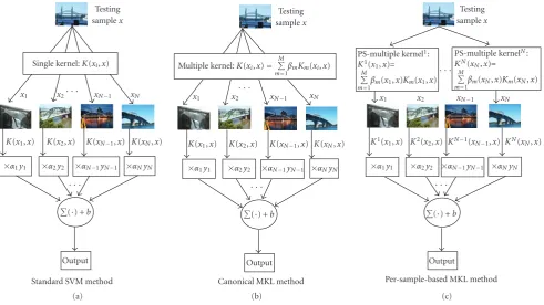
Figure2: Three paradigms of learning visual concepts from images using: (a) Standard SVM method; (b) Canonical MKL method; (c) PS-MKL method.

in an unseen image. Three layers are involved, that is, input layer, middle layer, and decision layer. Three methods adopt a similar framework but differ in kernel structure. In the input layer,xrepresents a test sample to be fed into a kernel-based classifier. In the middle layer, the similarities between a test sample x and training samples{xi}Ni=1 are measured

via different kernel structures, respectively. As shown in

Figure 2(a), a standard SVM method employs a single kernel to measure the sample similarity. But both canonical MKL (see Figure 2(b)) and PS-MKL (see Figure 2(c)) combine multiple basic kernels to measure the similarities between samples. A canonical MKL employs a uniform multiple kernel combination whereas PS-MKL employs a sample-wise kernel combination. In PS-MKL, the kernel weights not only depend on basic kernel functions, but also on each sample pair to compare. In the bottom layer, a decision function is used to determine whether a test samplexcontains a given concept.

In this section, we first briefly review a standard SVM and a canonical MKL in Section 3.1andSection 3.2. And then PS-MKL is presented inSection 3.3.

3.1. A Standard SVM. A standard SVM sets up a separating hyperplane to classify samples where a feature mapφ(x) is employed to project the original data from an input space to a feature space. To avoid an explicit representationφ(x) of the feature space, a so-called “kernel trick” is applied to define a kernel functionK(xi,xj) = φ(xi),φ(xj). For

binary classification, the decision function of a standard SVM is expressed as follows:

f(x)= N

i=1

αiyiK(xi,x) +b, (1)

where K(·,·) is a positive semidefinite kernel function associated with a reproducing kernel Hilbert space (RKHS), {αi}Ni=1andbare the classifier parameters to learn fromL.

3.2. A Canonical MKL. It is well known that SVM is an efficient tool for solving a classification problem. However, its discriminative power heavily depends on the kernel function which is at most cases selected by cross-validation. Instead of using a single kernel, MKL [9] learns a linear kernel combination and the associated classifier simultaneously. In a canonical MKL, the multikernel combination is defined as

K(xi,x)= M

m=1

βmKm(xi,x) (2)

with Mm=1βm = 1 andβm ≥ 0 for allm, where Km(·,·) is a positive semidefinite kernel function (referred to as a basic kernel), M is the total number of basic kernels, and {βm}Mm=1are kernel weights to optimize during training. Each

For binary classification, the decision function of a canonical MKL is given as follows:

f(x)= N

i=1

αiyi M

m=1

βmKm(xi,x) +b, (3)

where {αi}Ni=1 and b are the classifier parameters like the

parameters of decision function in a standard SVM. In MKL, the coefficients{αi}Ni=1and the kernel weights{βm}Mm=1can be

learnt by solving a joint optimization problem. Readers are referred to [9,30,31] for more details.

3.3. The Proposed PS-MKL. Instead of a uniform kernel combination in a canonical MKL, we propose a sample-based formulation of MKL, namely, PS-MKL.

In PS-MKL, the uniform multikernel combination in (2) can be rewritten as

K(xi,x)= M

m=1

βm(xi,x)Km(xi,x), (4)

whereβm(xi,x)is asample-wise kernel weightwith respect to

xiandx, rather than a fixedβmin a canonical MKL. Then the decision function in (3) can be reformulated as

f(x)= N

i=1

αiyi M

m=1

βm(xi,x)Km(xi,x) +b. (5)

Accordingly, our goal is to optimize the coefficientsα and thesample-wise kernel weightsβso as to construct a decision functionf(x).

It is worth to note that a basic kernel Km(xi,x) can utilize distinct feature setsxiandxto represent the similarity of images in different visual features. Basic kernels can take different kernel functions. In addition to the classical kernels (e.g., Gaussian and polynomial kernels) with dif-ferent parameters, several specific kernels in image domain (e.g., SPK [7] and PDK [28]) are often preferred. Further details on basic kernels are discussed in the experiments (See

Section 6.2).

4. Learning PS-MKL

In this section, we present how to learn the parameters of PS-MKL. In Section 4.1, we briefly describe the PS-MKL primal problem which is in spirit similar to the SVM primal problem. The consequent dual problem is described in Section 4.2, and the learning procedure is detailed in

Section 4.3.

4.1. The PS-MKL Primal Problem. In PS-MKL, a samplex

is translated by a feature mapping{φm(x)→RDm_}M m=1from

an input space toMfeature spaces (φ1(x),. . .,φM(x)), where

Dmdenotes the dimensionality of themth feature space. Each feature map is associated with a weight vector wm. So we have the linear combination of those corresponding output functions:

f(x)= M

m=1

βm(x)

wm,φm(x)

+b, (6)

whereβm(x) is a mixing coefficient to count the contribution

of feature mapφm(x) for the classification task.

Inspired by the standard SVM learning process, training can be implemented by solving the following optimization problem which involves maximizing the margin between positive/negative training samples as well as minimizing the classification error:

min β,w,b,ξ

1 2

M

m=1

wm2+C N

i=1

ξi,

s.t. yi ⎛ ⎝M

m=1

βm(xi)wm,ϕm(xi)+b

⎞

⎠_≥1−ξi,

ξi≥0,∀i, M

m=1

βm(x)=1, βm(x)≥0,∀m,

(7)

wherewm2is a regularization term that is inversely related to the margin,Ni=1ξimeasures the total classification error, and C is a tuning parameter to seek a tradeoff between margin maximization and classification error minimization. The L1regulation onβis meant to promote the sparsity of

sample-wise kernel weights.

4.2. The PS-MKL Dual Problem. By introducing Lagrange multipliers{αi}Ni=1into the inequality constraints in (7), we

can formulate a Lagrangian dual function that satisfies the Karush-Kuhn-Tucker (KKT) conditions [30]. Correspond-ingly, the PS-MKL primal problem is finally formulated as a max-min problem:

max β minα J

J= 1 2

N

i=1

N

j=1

αiαjyiyj ⎛ ⎝M

m=1

βm

xi,xj

Km

xi,xj ⎞

⎠

− N

i=1

αi,

s.t.

N

i=1

αiyi=0, 0≤αi≤C,∀i,

M

m=1

βm

xi,xj

=1, βm

xi,xj

≥0,∀i,∀j,∀m.

(8)

This max-min problem is subsequently called as a PS-MKL dual problem. Different fromβmin the canonical MKL dual problem [30], βm(xi,xj) in our PS-MKL dual problem is sample-wise. That is, the value ofβm(xi,xj) not only depends on the kernel functionKm(xi,xj), but also on the sample pair

xiandxj.

global classification error and maximize the inter-class

intervals. When α is fixed, maximizing J(·) over sample-wise kernel weights β is meant to maximize the global

intra-classsimilarity and minimize theinter-classsimilarity simultaneously. Solving this Max-Min problem is a typical saddle point problem. We next present the solution.

4.3. An Efficient Learning Algorithm. Similar to the param-eter learning in a canonical MKL, we adopt a two-stage alternant optimization procedure.

4.3.1. The Computation ofαGiven a Fixedβ. Fixingβ, the classifier coefficients α can be estimated by minimizing J under the constraints of 0≤αi≤Cfor alliand

N i=1αiyi= 0. Minimization ofJis identical to solving a standard SVM dual problem with the kernel combination

Kxi,xj

= M

m=1

βm

xi,xj

Km

xi,xj

. (9)

So minimizing J over α can be easily accomplished by existing efficient SVM solvers.

4.3.2. The Computation of β Given a Fixed α. Fixing α, optimizing the sample-wise kernel weights βm(xi,xj) is to explore the individual contribution of a feature (or a basic kernel) to the classification, with respect to the sample-pair

xiandxj.

However, it is difficult to obtain an analytical solution about a generalized form of βm(xi,xj). For simplicity, we assume that βm(xi,xj) can be decoupled into βm(xi) and

βm(xj), whereβm(xi) depends on samplexiand themth basic kernel only, and similarly forβm(xj). Under this assumption,

βm(xi,xj) can be expressed asβm(xi). βm(xj) as mentioned in [32]. However, this optimization function is not convex. Alternatively, we define βm(xi,xj) = (βim +β

j

m)/2 in our work to preserve the convexity of the optimization function J, where βi

m corresponds to βm(xi). Then the sample-wise kernel weights can be expressed byβ =(β1,. . .,βn,. . .,βN) andβn=(βn

1,...,βnm,...,βnM)T, whereβnm∈R.

The learning process of our sample-wise kernel weights is different fromβm(xi,xj) used in the local MKL [32]. Firstly, the objective function in [32] is not convex when solving the optimization problem of kernel combination, thereby leading to a local optimum. Secondly, the optimization of kernel combination in [32] resorts to an explicit feature representation, which would be subject to the curse of dimensionality.

To optimize the sample-wise kernel weightsβwith fixed α, the objective function in (8) can be expressed as

Jβ= N

i=1

M

m=1

βimSim(α) + N

j=1

M

m=1

βmjSm(α)j − N

i=1

αi, (10)

where

Si m(α)=

1 4αiyi

N

j=1

αjyjKm

xi,xj

,

Sm(α)j = 1 4αjyj

N

i=1

αiyiKm

xi,xj

.

(11)

Without loss of generality, the objective function with respect toβcan be rewritten as

max β 2

N

i=1

M

m=1

βi

mSim(α)− N

i=1

αi, (12)

then the optimization ofJoverβturns to

max θ

w.r.t. θ∈R, β∈RN·K_,

s.t.2 N

i=1

M

m=1

βimSim(α)− N

i=1

αi≥θ,

M

m=1

βim=1, βim≥0,∀i,∀m,

∀α∈RN_{, with 0≤α} i≤C,

N

i=1

αiyi=0. (13)

Given fixed α, the optimization of J over β is a linear program (LP) problem as θ andβ are only linearly constrained. Nevertheless, the constraint onθ has to hold for every compatible α resulting from infinite constraints. To solve this so-called semiinfinite linear program (SILP) problem, a column generation strategy is employed. That is, by solving the former QP with fixedβwe produce a special α, which then adds a constraint onθ. In this way we add new constraints iteratively and consequently solve the LP with the help of all the gained constraints. This procedure has been proven to converge in [33].

In summary, we solve the saddle point problem by two alternant processes: (1) using an off-the-shelf SVM solver to learn the classifier coefficientsαand (2) using the simplex LPs to learn sample-wise kernel weightsβ. In the training phase, sample-wise kernel weights of the training samples are leant by optimizing the object function J(β).

Uncertain data Unlabeled data pool

PS-MKL classifier

Initial training data Filtering

Clustering

Testing Training Training Batch data

Labeling User Labeling

Sample selection The informative score ranking Group1

data · · ·

Groupk data

Figure3: The flowchart of sample selection for PS-MKL.

4.3.3. Learning Algorithm for PS-MKL. The optimization algorithm of PS-MKL is summarized in Algorithm 1. The termination criteria can be the consistency of α or β between two consecutive steps, or a predefined iteration upper bound. Optimizing the classifier coefficients and the sample-wise kernel combination is a linear programming wrapping canonical SVM solver process.

5. Sample Selection for PS-MKL

In PS-MKL, the computational complexity involves two major processes: (1) computing multiple kernel functions for each sample-pair over the training set and (2) optimizing the classifier parameters and the sample-wise kernel weights in an alternate manner, which incurs intensive computation for an optimal solution. In particular, as the size of training set increases, the higher complexity of learning parameters would be a bottleneck in efficiently training PS-MKL. Intuitively, there would probably exist considerable data redundancy in a large-scale training dataset. By removing redundant data and keeping informative samples, we can reduce the size of actually used training data while the classifier’s discriminative power is kept comparable.

In the community of machine learning, active learning is one of widely used techniques to reduce the labeling cost in supervised learning tasks. That is, by repeatedly querying the unlabeled samples, we may select the most informative samples to label, so that the demand for a large quantity of labeled data is alleviated [34]. In this paper, we incorporate the process of active learning into PS-MKL to select informative training samples for training. Accordingly, the calculation of kernel matrices, the learning of sample-wise kernel combination and a kernel-based classifier can be conducted over those selected samples only. So the computational complexity is reduced.

Figure 3illustrates the basic process. Firstly, a prelimi-nary PS-MKL classifier is trained on an initial labeled dataset. Secondly, the images from an unlabeled data pool will be filtered by the learnt classifier, collecting uncertain samples for further selection. Thirdly, these uncertain samples will go through sample selection to give a batch of most informative samples. Fourthly, a retraining of the classifier continues on the batch of data, together with the initial training data, to refine its discriminative power. Then the active learner jumps to the second step and continue.

5.1. Filtering in Uncertain Samples. Given an initial PS-MKL classifier learnt from a small labeled dataset L, our sample selection aims to collect unused samples that are uncertainfor the classifier as the candidates of informative samples. These samples could be useful to further improve the classifier [35].

For each input, we can get an output score through computing the decision function of PS-MKL. This score indicates the likelihood that the input sample belongs to a given concept. Moreover, it ranks input samples by the likelihood of an instance belonging to a concept. In a sense, we may think the decision function transforms the original feature space into one-dimensional output score space, and establishes the ordered probabilities of a sample belonging to a concept. Hence, we select theuncertain samplesaccording to the output score f(x) of the PS-MKL:

Unc(x)= ⎧ ⎨ ⎩

1 ifT−≤ f(x)≤T+_,

0, otherwise, (14)

where T−and T+_{are the negative and positive bounds,}

respectively. These two bounds can be predefined or empiri-cally estimated by a heuristic rule.

5.2. Selecting Informative Samples. To reduce the iterations of active learning, we adopt a batch mode to do sample selection. In each iteration, the uncertain samples are first clustered into groups, so that visually similar samples are merged into a group. Then the most informative samples in each group are added into the small labeled datasetLfor classifier updating. K-means is utilized in our work, where other clustering methods can also be applied.

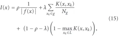
Within each group, we sort the candidate samples by three criteria: (1) the distance of a sample from the classifica-tion boundary, (2) the representativeness of a sample within the group, and (3) how distinguished a sample is from the training samples ofL. The informative scoreI(x) of a sample

xcan be computed as

I(x)=ρ 1 f(x)+λ

xk∈g

K(x,xk)

Ng

+ 1−ρ−λ

1−max

xk∈LK(x,xk)

,

(15)

whereρandλare two parameters to weight the importance of three components; |f(x)| is the distance from the classification boundary;g denotes the group that samplex

belongs to;Ng is the number of samples within the group

g;K(x,xk) represents the similarity between sample x and

Initt=1, βi

m=1/M, ∀i∀m

whilethe termination criterion NOT metdo

(a) Compute the classifier coefficientsαt_{by a standard}

SVM to solve the problem:

αt_{=arg min}

α

1 2

N

i=1 N

j=1

αiαjyiyjK(xi,xj)− N

i=1

αi

s.t.N

i=1αiyi=0, 0≤αi≤C, ∀i.

withK(xi,xj)=

M

m=1βm(xi,xj)Km(xi,xj).

(b) Update the object function

Jt₌₂N i=1

M

m=1

βi

mSim(αt)− N

i=1

αt i,

whereSi m(αt)=

1 4α

t iyi

N

j=1

αt

jyjKm(xi,xj).

(c) Compute the kernel weightsβby (β,θ)=arg maxθ

w.r.t.β∈RN·K_{, θ∈R}

s.t.M

m=1β i

m=1,βim≥0, ∀i,∀m

2

N

i=1 M

m=1

βi

mSim(αh)− N

i=1

αh

i ≥θ, forh=1,· · ·t.

(d) t=t+ 1

end while

Compute the bias of the decision function (5) by

b=yj− N

i=1

αt−1 i yi

M

m=1

βm(xi,xj)Km(xi,xj), ∀j∈ {j|αtj−1>0}.

Algorithm1: PS-MKL optimization process.

6. Experiments

6.1. Datasets. Extensive experiments are performed on three well-known benchmarking datasets, that is, Caltech101 [15], WikipediaMM [16], and Pascal VOC’07 [17]. Caltech101 involves 102 object categories, each category containing 31 to 800 images. In WikipediaMM, some 150,000 images on diverse topics are crawled from Wikipedia. Our experiments select 33 topics, each of which has more than 80 positive samples. Pascal VOC’07 consists of 20 object categories from real-world images, where 2501 images are used for training, 2510 images for validation, and 4952 images for test. Our primary goal is to investigate the effectiveness of PS-MKL on open benchmarking data sets for fair comparisons with previous work. In addition, we consider the WikipediaMM from the multimedia community, which is to evaluate PS-MKL over a real-world data from a practical retrieval point of view, and how the performance of concept learning changes with the problem complexity. For each dataset, the one-vs.-allsetting is adopted for training multiple classifiers of visual concepts.

6.2. Features and Kernels. Two local appearance features (dense-color-SIFT (DCSIFT) and dense-SIFT (DSIFT) [7]) and two shape features (self-similarity (SS) [36] and pyra-mid histogram of orientated gradients (PHOGs) [29]) are utilized. DCSIFT is computed in CIE-lab 3-channels over a square patch of radii r with the spacing of r. We use

r =4, 8, and 12 pixels to allow some scalability. In a similar manner, DSIFT is calculated in a gray image. SS descriptor captures the correlation map of a set of 5×5 patches with their neighbors at every 5th pixel. The correlation map is quantized into 10 orientations and 3 radial bins so as to form a 30 dim descriptor. Based on dense features, we employ k-means to quantize these three descriptors to obtain three codebooks of size k (set as 400, cf. [7]), respectively. For PHOG, two spatial pyramid kernels of gradient orientation are calculated to measure the image similarity in shape. We use the same PHOG setting as [29], that is, 20 orientation bins for PHOG-180 degree and 40 bins for PHOG-360 degree.

We implement SPK [7] and PDK [28]. For SPK, an image is divided into cells and a feature similarity from spatially corresponding cells between images is measured. The resulting kernel is formed as a weighted combination of histogram intersections from coarse cells to fine cells. A 4-level pyramid is used with the grid sizes of 8 × 8, 4 × 4, 2 × 2, and 1 × 1, respectively. For PDK, the local feature distributions of the K-nearest neighbors are compared between images. The resulting kernel combines the local feature distributions at multiple scales, for example,

Table1: Mean recognition rates of four multiple kernel-based methods on Clatech101.

Methods Number of positive samples for training

5 10 15 20 25 30

UMK 56.21 65.16 68.38 70.47 71.26 72.69

MKL 55.30 66.45 70.76 73.62 74.73 75.35

PS-MKL 58.59 69.24 74.82 77.37 79.41 80.67

PS-MKL-SS 58.59 70.02 76.63 79.74 80.91 81.82

Table2: Comparison of four multiple kernel-based methods on WikiPediaMM by using Mean Average Precision as metric.

Methods Number of positive samples for training

5 10 15 20 25 30

UMK 34.32 38.87 42.04 44.78 47.02 49.21

MKL 38.79 45.03 50.08 54.31 56.14 58.17

PS-MKL 40.63 47.14 53.67 57.53 59.82 61.36

PS-MKL-SS 40.63 51.35 57.54 61.34 62.23 64.84

6.3. Experiment Result

6.3.1. Experiments on Caltech101

Comparison with Different Multiple Kernel Methods. We compare the performance of four multiple kernel meth-ods with the same setting of training/testing partition. Unweighted multiple kernel (UMK) method applies equal kernel weights to different basic kernels. Canonical MKL is implemented by the Matlab code from [30]. PS-MKL is implemented as introduced in Section 4. PS-MKL-SS employs the sample selection strategy inSection 5, while the other three methods apply a random sampling strategy. The mean recognition rates of four methods on Caltech101 are listed inTable 1. We adopt the same experimental setting as reported in state-of-the-art works [7,8,10,14,15,18,19,21,

37–40], where different numbers of positive samples, that is,

Ntrain={5, 10, 15, 20, 25, 30}are applied to the training phase

and a fixed number of samples (Ntest=30) are applied to test

phase for each concept.

Compared with UMK and MKL, PS-MKL achieves different improvements over all the training setting as shown inTable 1. We also observe that the sample selection further improves the performance of PS-MKL and obtains the best performance among four multiple kernel methods. Note that with a smaller training set Ntrain = 20, PS-MKL-SS

has achieved promising MAPs comparable to that of PS-MKL at Ntrain = 30. Through comparisons, our proposed

sample selection method is also shown to be more effective than a random sampling strategy in UMK, MKL, and PS-MKL.

Comparison with Other Methods. On Caltech101, we com-pare PS-MKL with other types of recent methods [7,8,10,

14,15,18,19,21,37–40]. For each concept, we randomly select Ntrain and Ntest positive images to perform one-vs.-alltraining and testing at different training set sizes, where

Ntrain = {5, 10, 15, 20, 25, 30} andNtest = 15. As shown

in Figure 4, our approach has achieved promising results

0 10 20

M

ean

re

co

gnition

rat

e

p

er

class

30 40 50 60 70 80 90

0 5 10 15 20 25 30 35 40 45 50

Number of training examples per class Comparison on Caltech101

Varma et al. (ICCV2007) PS-MKL

Todorovic et al. (CVPR2008) Bosch et al. (ICCV2007) Gehler et al. (ICCV2009) Frome et al. (ICCV2007) Zhang et al. (CVPR2006)

Giffin et al. (tech Rep,2007) Lazebnik et al. (CVPR2006) Wang et al. (CVPR2006) Kumar et al. (ICCV2007) Mutch et al. (CVPR2006) Fei-Fei et al. (2004) Figure4: Performances of PS-MKL and other types of methods on Caltech101, with the PS-MKL figures of: 5(58.59), 10 (69.24), 15 (74.82), 20 (77.37), 25 (79.41), 30 (80.67) as (positive training sample number, mean recognition rate).

comparable to the top performances. WhenNtrain = 30, the

mean recognition rate of PS-MKL reaches up to 80.67%. As a multiple kernel-based method, the approach of Varma and Ray [8] got the best result on Caltech 101, with a recognition rate of 87.82% when Ntrain = 15. Both

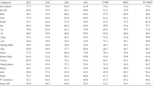
Table3: Average Precision of PS-MKL and other methods on the Pascal VOC 2007 dataset.

Categories [41] [24] [42] [43] UMK MKL PS-MKL

Aero plane 77.5 63.0 65.0 65.0 72.9 74.1 75.0

Bicycle 63.6 22.0 44.3 48.0 52.2 53.9 54.0

Bird 56.1 14.0 48.6 44.0 47.0 46.6 48.6

Boat 71.9 42.0 58.4 60.0 61.8 62.2 65.2

Bottle 33.1 43.0 17.8 20.0 33.5 37.5 41.6

Bus 60.6 50.0 46.4 49.0 49.0 55.6 57.7

Car 78.0 62.0 63.2 70.0 69.5 70.7 71.9

Cat 58.8 32.0 46.8 49.0 45.8 48.4 48.4

Chair 53.5 37.0 42.2 50.0 53.2 54.0 59.0

Cow 42.6 19.0 29.6 32.0 32.7 34.7 36.8

Dining table 54.9 30.0 20.8 39.0 48.3 50.1 52.1

Dog 45.8 29.0 37.7 40.0 44.2 40.7 46.7

Horse 77.5 15.0 66.6 72.0 70.3 76.6 72.6

Motor-bike 64.0 31.0 50.3 59.0 55.0 59.8 63.6

Person 85.9 43.0 78.1 81.0 85.1 82.5 86.5

Potted plant 36.3 33.0 27.2 32.0 32.4 38.3 44.3

Sheep 44.7 41.0 32.1 35.0 36.8 40.0 43.0

Sofa 50.6 37.0 26.8 42.0 45.9 48.2 54.2

Train 79.2 29.0 62.8 68.0 67.5 68.1 70.1

TV monitor 53.2 62.0 33.3 49.0 47.5 47.2 49.2

Mean AP 59.4 36.7 44.9 50.2 52.5 54.5 57.0

DCSIFT, PHOG180, and PHOG 360) are incorporated into an extended MKL framework.

6.3.2. Experiments on WikiPediaMM. Now let us evaluate the multiple kernel-based methods (i.e., UMK, MKL, PS-MKL, and PS-MKL-SS) on WikipediaMM. For each visual concept, we perform six runs with Ntrain ={5, 10, 15, 20,

25, 30}positive image samples forone-vs.-alltraining, while the rest of positive images are used for test. The mean of average precisions (MAPs) [16] for six runs are listed in

Table 2. At the same empirical setting, PS-MKL outperforms UMK and MKL. That is, even on the large-scale image corpus in practice, PS-MKL shows stronger discriminative power.

From Table 2, we observe that PS-MKL-SS achieves

improvements over PS-MKL with more sampling images in each round. At a smaller training sizeNtrain = 20,

PS-MKL-SS has achieved an MAP 61.34%, which is comparable to the best result of PS-MKL (MAP 61.36% at Ntrain =

30). Beyond PS-MKL, PS-MKL-SS not only achieves better results, but also is able to get comparable performance with less training samples and comparatively lower computation. So our proposed PS-MKL equipped with a sample selection is more effective and efficient.

To illustrate the effects of PS-MKL on WikipediaMM, we list the top correctly returned positive and negative images of ten concepts in Figure 5. With a finer category, some negative and positive images of a concept not only have similar appearances, but also produce semantic correlations,

for example, hunting dog versus pet dog, and race car versus vehicle, whereas our PS-MKL works well.

6.3.3. Experiments on Pascal VOC’07. For each concept, we employ 5011 images for training and 4952 images for test.Table 3compares the performances of PS-MKL to two multiple kernel methods (UMK and MKL) and other recent methods [24,41–43]. An official performance metric Average Precision (AP) [17] is used.

At the same setting of training/testing sets, PS-MKL has obtained relative improvements of 7.9% and 4.4% over UMK and MKL. More or less improvements have been achieved over all 20 concepts. In particular, “chair” and “potted plant” receive over 10% improvements. By investigating the intra-class diversity of each concept in Pascal VOC’07, we find that PS-MKL allows better discriminative power than UMK and MKL in the dataset.

FromTable 3, PS-MKL has achieved a promising MAP

57.0%, which is better than [24,42,43], and the performance is very close to the best reported performance (MAP 59.4% in [41]) in Pascal VOC’07 challenge.

P1 P2 P3 N1 N2

B

ridges

Ci

ti

es

b

y

nig

ht

F

o

otball

stadium

Hi

st

o

ri

c

castle

Ho

u

se

ar

ch

it

ectur

e

(a)

P1 P2 P3 N1 N2

H

u

nting _dog

Mo

u

n

ta

in

and

sky

Rac

e

car

Star _galax

y

Mi

li

ta

ry

air

cr

aft

(b)

Figure5: Illustration of top three positive and top two negative samples of correctly returned results on WikipediaMM dataset.

SILP. The time complexity of SILP is ignorable compared to the SVM solver. Using hot start (i.e., providing previousαas an initial input) can accelerate the process of SVM solvers. In the case of learning a concept from 5 k samples on Pascal VOC’07, training a canonical MKL takes some 12 minutes, and PS-MKL needs about 30 minutes to converge for each concept. To compute the decision function during test, we need to calculate the kernel functionKm(xi,x) only whenαi andβi

mare nonzero.

7. Discussion

Through working across multiple basic kernel spaces, PS-MKL helps to capture the intra-class diversity of a visual concept. When a canonical MKL method is deficient in dealing with the intra-class diversity using uniform kernel combination, PS-MKL may provide a tractable approach to kernel weighting at the sample level. Our experiments show that PS-MKL achieves significant improvements over a canonical MKL method.

Like other sample-based methods, PS-MKL has to opti-mize numerous parameters especially when massive training samples are available. For example, in Caltech101, 8 basic kernels and 30 training samples per class lead to some 25 k sample-wise kernel weights. Since the number of classifier parameters is in proportion to the number of (sparse) support vectors, there are only 1∼3 k nonzero sample-wise kernel weights to optimize, and then PS-MKL is tractable. In practice, however, when the number of training samples keeps growing, how to solve PS-MKL efficiently would become a critical problem.

In another work [44], we extend PS-MKL and present a group-sensitive multiple kernel learning method

(GS-MKL). In GS-MKL, an intermediate representation “group” is introduced between object categories and individual images to seek a tradeoff between capturing the diversity and keeping the invariance for each category. Visually similar training samples within a group are assigned a uniform kernel combination, while distinct training samples may have different kernel combinations. Hence, the number of kernel weights can be greatly reduced by allowing visually similar training samples to share a kernel combination setting.

How to make the optimal allocation of different ker-nel combinations over more complex training samples is included in our future work to take into account more practical issues such as a discriminative power and a reduced classifier complexity.

8. Conclusion

Acknowledgments

The work is supported by grants from the Chinese National Natural Science Foundation under Contract no. 60605020, no. 60973055, no. 60902057, and no. 90820003, The National Hi-Tech R and D Program (863) of China under Contract 2006AA010105, and the National Basic Research Program of China under Contract no. 2009CB320906. This work was performed when Jingjing Yang and Yuanning Li were visiting NELVT as full-time research assistant.

References

[1] M. Szummer and R. W. Picard, “Indoor-outdoor image classification,” inProceedings of the International Workshop on Content-Based Access of Image and Video Databases, 1998. [2] J. Vogel and B. Schiele, “Natural scene retrieval based on a

semantic modeling step,” inProceedings of the International Conference on Image and Video Retrieval, pp. 207–215, 2004. [3] J. Sivic, B. C. Russell, A. A. Efros, A. Zisserman, and W. T.

Freeman, “Discovering objects and their location in images,” inProceedings of the 10th IEEE International Conference on Computer Vision (ICCV ’05), vol. 1, pp. 370–377, Beijing, China, October 2005.

[4] R. Fergus, L. Fei-Fei, P. Perona, and A. Zisserman, “Learning object categories from Google’s image search,” inProceedings of the 10th IEEE International Conference on Computer Vision (ICCV ’05), vol. 2, pp. 1816–1823, Beijing, China, October 2005.

[5] A. W. M. Smeulders, M. Worring, S. Santini, A. Gupta, and R. Jain, “Content-based image retrieval at the end of the early years,” IEEE Transactions on Pattern Analysis and Machine Intelligence, vol. 22, no. 12, pp. 1349–1380, 2000.

[6] K. Q. Weinberger, J. Blitzer, and L. K. Saul, “Distance metric learning for large margin nearest neighbor classification,” in

Advances in Neural Information Processing Systems, 2005. [7] S. Lazebnik, C. Schmid, and J. Ponce, “Beyond bags of

features: spatial pyramid matching for recognizing natural scene categories,” inProceedings of the IEEE Computer Society Conference on Computer Vision and Pattern Recognition (CVPR ’06), vol. 2, pp. 2169–2178, New York, NY, USA, June 2006. [8] M. Varma and D. Ray, “Learning the discriminative

power-invariance trade-off,” in Proceedings of the 11th IEEE Inter-national Conference on Computer Vision (ICCV ’07), Rio de Janeiro, Brazil, October 2007.

[9] F. R. Bach, G. R. G. Lanckriet, and M. I. Jordan, “Multiple kernel learning, conic duality, and the SMO algorithm,” in

Proceedings of the 21st International Conference on Machine Learning (ICML ’04), pp. 41–48, July 2004.

[10] A. Kumar and C. Sminchisescu, “Support Kernel machines for object recognition,” in Proceedings of the 11th IEEE International Conference on Computer Vision, 2007.

[11] J. Platt, “Fast training of support vector machines using sequential minimal optimization,” in Advances in Kernel Methods: Support Vector Learning, pp. 185–208, MIT Press, Cambridge, Mass, USA, 1998.

[12] O. Chum and A. Zisserman, “An exemplar model for learning object classes,” in Proceedings of the IEEE Computer Society Conference on Computer Vision and Pattern Recognition, June 2007.

[13] A. Frome, Y. Singer, F. Sha, and J. Malik, “Learning globally-consistent local distance functions for shape-based image retrieval and classification,” in Proceedings of the 11th IEEE

International Conference on Computer Vision, Rio de Janeiro, Brazil, 2007.

[14] T. Malisiewicz and A. A. Efros, “Recognition by association via learning per-exemplar distances,” inProceedings of the 26th IEEE Conference on Computer Vision and Pattern Recognition (CVPR ’08), June 2008.

[15] L. Fei-Fei, R. Fergus, and P. Perona, “Learning generative visual models from few training examples: an incremental Bayesian approach tested on 101 object categories,” inProceedings of the Computer Vision and Pattern Recognition (CVPR ’04), 2004.

[16] http://www.imageclef.org/2008/wikipedia.

[17] M. Everingham, L. VanGool, C. K. I. Williams, J. Winn, and A. Zisserman, “The PASCAL visual object classes challenge 2007 (VOC2007) results,”

http://pascallin.ecs.soton.ac.uk/challenges/VOC/voc2007/

workshop/index.html.

[18] S. Fidler, M. Boben, and A. Leonardis, “Similarity-based cross-layered hierarchical representation for object categorization,” inProceedings of the 26th IEEE Conference on Computer Vision and Pattern Recognition (CVPR ’08), June 2008.

[19] A. Bosch, A. Zisserman, and X. Mu˜noz, “Image classification using random forests and ferns,” inProceedings of the 11th IEEE International Conference on Computer Vision (ICCV ’07), October 2007.

[20] J. Yang, Y. Li, Y. Tian, L. Duan, and W. Gao, “A new multiple kernel approach for visual concept learning,” inProceedings of the 15th International Multimedia Modeling Conference, pp. 250–262, 2009.

[21] Y.-Y. Lin, T.-L. Liu, and C.-S. Fuh, “Local ensemble kernel learning for object category recognition,” inProceedings of the IEEE Computer Society Conference on Computer Vision and Pattern Recognition, 2007.

[22] D. Crandall, P. Felzenszwalb, and D. Huttenlocher, “Spatial priors for part-based recognition using statistical models,” in Proceedings of the IEEE Computer Society Conference on Computer Vision and Pattern Recognition, vol. 1, pp. 10–17, June 2005.

[23] L. Fei-Fei, R. Fergus, and P. Perona, “One-shot learning of object categories,”IEEE Transactions on Pattern Analysis and Machine Intelligence, vol. 28, no. 4, pp. 594–611, 2006. [24] C. Galleguillos, A. Rabinovich, and S. Belongie, “Object

categorization using co-occurrence, location and appearance,” inProceedings of the 26th IEEE Conference on Computer Vision and Pattern Recognition (CVPR ’08), June 2008.

[25] A. Ng and M. Jordan, “On discriminative vs. generative classifiers: a comparison of logistic regression and naive Bayes,” inAdvances in Neural Information Processing Systems, 2002.

[26] J. Shawe-Taylor and N. Cristianini,Kernel Methods for Pattern Analysis, Cambridge University Press, Cambridge, Mass, USA, 2004.

[27] K. Grauman and T. Darrell, “The pyramid match kernel: discriminative classification with sets of image features,” in

Proceedings of the 10th IEEE International Conference on Computer Vision, vol. 2, pp. 1458–1465, Beijing, China, October 2005.

[28] H. Ling and S. Soatto, “Proximity distribution kernels for geometric context in category recognition,” inProceedings of the 11th IEEE International Conference on Computer Vision, 2007.

[30] S. Sonnenburg, G. Raetsch, C. Schaefer, and B. Scholkopf, “Large scale multiple kernel learning,” Journal of Machine Learning Research, vol. 7, pp. 1531–1565, 2006.

[31] A. Rakotomamonjy, F. R. Bach, S. Canu, and Y. Grandvalet, “SimpleMKL,”Journal of Machine Learning Research, vol. 9, pp. 2491–2521, 2008.

[32] M. G¨onen and E. Alpaydin, “Localized multiple kernel learning,” inProceedings of the 25th International Conference on Machine Learning, pp. 352–359, July 2008.

[33] S. Sonnenburg, G. Ratsch, and C. Schafer, “A general and efficient multiple kernel learning algorithm,” inNeural Infor-mation Processing Systems, 2005.

[34] S. Tong and D. Koller, “Support vector machine active learning with applications to text classification,”The Journal of Machine Learning Research, vol. 2, pp. 45–66, 2002.

[35] S. C. H. Hoi, J. Zhu, R. Jin, and M. R. Lyu, “Semi-supervised SVM batch mode active learning for image retrieval,” in

Proceedings of the 26th IEEE Conference on Computer Vision and Pattern Recognition, 2008.

[36] E. Shechtman and M. Irani, “Matching local self-similarities across images and videos,” inProceedings of the IEEE Computer Society Conference on Computer Vision and Pattern Recogni-tion, 2007.

[37] H. Zhang, A. C. Berg, M. Maire, and J. Malik, “SVM-KNN: discriminative nearest neighbor classification for visual cate-gory recognition,” inProceedings of the IEEE Computer Society Conference on Computer Vision and Pattern Recognition, vol. 2, pp. 2126–2136, June 2006.

[38] G. Wang, Y. Zhang, and L. Fei-Fei, “Using dependent regions for object categorization in a generative framework,” in Pro-ceedings of the IEEE Computer Society Conference on Computer Vision and Pattern Recognition, vol. 2, pp. 1597–1604, 2006. [39] J. Mutch and D. G. Lowe, “Multiclass object recognition

with sparse, localized features,” in Proceedings of the IEEE Computer Society Conference on Computer Vision and Pattern Recognition, vol. 1, pp. 11–18, 2006.

[40] P. Gehler and S. Nowozin, “On feature combination for multiclass object classification,” in Proceedings of the IEEE International Conference on Computer Vision, 2009.

[41] M. Marszałek, C. Schmid, H. Harzallah, and J. Weijer, “Learn-ing object representations for visual object class recognition,” inProceedings of the Visual Recognition Challenge Workshop, in Conjunction with IEEE International Conference on Computer Vision, 2007.

[42] G. Wang, D. Hoiem, and D. Forsyth, “Learning image simi-larity from Flickr groups using stochastic intersection kernel machines,” inProceedings of the of International Workshop on Multimedia Information Retrieval, 2008.

[43] F. Khan, J. Weijer, and M. Vanrell, “Top-down color attention for object recognition,” inProceedings of the IEEE International Conference on Computer Vision, 2009.