Meta analysis of binary data with excessive zeros in two-arm trials

R E S E A R C H

Open Access

Meta analysis of binary data with

excessive zeros in two-arm trials

Saman Muthukumarana

, David Martell

and Ram Tiwari

*Correspondence:

[email protected] 1_{Department of Statistics, University}

of Manitoba, Machray Hall, Winnipeg, Canada

Full list of author information is available at the end of the article

Abstract

We present a novel Bayesian approach to random effects meta analysis of binary data with excessive zeros in two-arm trials. We discuss the development of likelihood accounting for excessive zeros, the prior, and the posterior distributions of parameters of interest. Dirichlet process prior is used to account for the heterogeneity among studies. A zero inflated binomial model with excessive zero parameters were used to account for excessive zeros in treatment and control arms. We then define a modified unconditional odds ratio accounting for excessive zeros in two arms. The Bayesian inference is carried out using Markov chain Monte Carlo (MCMC) sampling techniques. We illustrate the approach using data available in published literature on myocardial infarction and death from cardiovascular causes. Bayesian approaches presented here use all the data, including the studies with zero events and capture heterogeneity among study effects, and produce interpretable estimates of overall and study-level odds-ratios, over the commonly used frequentist’s approaches. Results from the data analysis and the model selection also indicate that the proposed Bayesian method, while accounting for zero events, adjusts for excessive zeros and provides better fit to the data resulting in the estimates of overall odds-ratio and study-level odds-ratios that are based on the totality of the information.

Keywords: Dirichlet process, Model selection, Markov chain Monte Carlo, Simulation

1 Introduction

An arm is a standard term for describing clinical trial and it represents a treatment group or a set of subjects. A two-arm study compares a drug with a placebo or drug A with drug B. Sometimes in these studies, the outcome may be binary. A binary outcome is an outcome whose unit can take on only two possible states “0" and “1". For example, out-comes of clinical trials data such as the morbidity and mortality studies are often binary in nature.

The natural distribution for modeling these types of binary data is the binomial distribution given by

f(y;p)=

n y

py(1−p)n−y for y=0, 1,. . .,n, p∈(0, 1).

The mean and variance for the binomial random variable areE(Y) = npandVar(Y) = np(1−p)respectively. In a two-arm trial with binary outcomes, it is typically assumed thatYT1, ...,YTkandYC1, ...,YCk are random samples fromYTi∼ Bin

nTi,PTi

andYCi ∼

BinnCi,PCi

respectively, wherekis the number of studies. In a random effects meta

analysis of these types of data, the effect size is assumed to vary from study to study. Random effects meta analysis assumes that study effects are a random sample from an underlying relevant distribution of effects, and the combined effect estimates the mean effect of this distribution.

There are a variety of different approaches to analyze these types of data as indicated by some recent literature. See Albert (1995) for various parametrization of binomial models for discrete data within Bayesian settings. Chang et al. (2001) use a mixed effects model to investigate between and within-study variation using rate difference and logit models. Gamalo et al. (2011) propose a Bayesian procedure for testing noninferiority in two-arm studies with a binary primary endpoint that allows the incorporation of historical data on an active control via the use of informative priors but did not consider excessive zeros. Carlin (1992) consider a Bayesian meta-analysis approach for two way contingency table data while Smith et al. (1995) discuss how a full Bayesian analysis can be used to deal with issues in meta-analysis in a natural way using the BUGS language. In this paper, we consider a Bayesian approach for binary data with excessive zeros in two-arm trials. More specifically, we model the excessive zeros using zero inflated binomial distribution and use the Dirichlet process Ferguson (1974) to handle the heterogeneity among studies. There are various zero inflated methods available in the literature. Hall (2000) introduced the framework for count data with many zeros using Poisson and binomial models and likelihood ratio tests based inference for zero inflated Poisson models are discussed in Huang et al. (2014). A Bayesian inference framework for zero inflated Poisson regression models is discussed in Ghosh et al. (2006). A rich class of nonparametric Bayesian priors for study effects and Bayesian nonparametric Polya tree mixture model are developed in Branscum and Hanson (2008) and Burr and Doss (2005).

In Section2, we describe Bayesian model specification used in the paper. The like-lihood function and the priors are described. Study effects have a Dirichlet process prior distribution for capturing heterogeneity among studies. We then obtain posterior summary statistics which describe key features in the model. In particular, posterior expectations are approximated through Markov chain Monte Carlo (MCMC) methods. In Section3, the model is applied to a large dataset available in the literature Nissen and Wolski (2007). We perform the model selection using the log-pseudo marginal like-lihood (LPML) comparing the Binomial and zero-inflated Binomial (ZIB). The results suggest that when the data has a high percentage of observed zeros, ZIB model is a more appropriate model to use. Furthermore, the use of Dirichlet process has advan-tage over the more commonly used random effects model with normally distributed random effects based on DerSimonian-Laird approach DerSimonian and Laird (1986) or a Bayesian approach using normal priors, in terms of its inherent clustering property resulting in the studies with similar effects to cluster, and thus providing more robust estimates. We also test the approach using simulation studies in Section4 and study the effect of excessive zeros in the ZIB models. We conclude with a short discussion in Section5.

2 Model development

Consider two-arm trials with binary outcomes and letYTi

ind

∼ BinnTi,PTi

andYCi

ind ∼

BinnCi,PCi

,i = 1,. . .,k, wherekis the number of studies. Then the joint likelihood

L=LyT1,. . .,yTk,yC1,. . .,yCk|μ,PT,PC

L=

k

i=1

n_TiC y_TiP

y_Ti

Ti(1−PTi)

n_Ti−y_Ti k

i=1

n_CiC y_CiP

y_Ci

Ci (1−PCi)

n_Ci−y_{Ci. (1)}

In random effects meta-analysis formulation, we assume thatPT andPC follow logistic

models, and define

PTi=

exp{μ+Tr+αi+ei}

1+exp{μ+Tr+αi+ei}andPCi=

exp{μ+ei}

1+exp{μ+ei}.

That is,logit(PTi)=μ+Tr+αi+ei;logit(PCi)=μ+ei,i=1,. . .,k. This gives,

logit(PTi)−logit(PCi)=Tr+αi;i=1,. . .,k,

where logit(p) = log ₁₋p_p

is the log-odds ratio of p, μ is the intercept, Tr

is the treatment effect, αi and ei are the study effects and error terms. As

pro-posed by Muthukumarana and Tiwari in Muthukumarana and Tiwari (2016), con-sider a Bayesian approach and assume that {αi;i=1,. . .,k} is a sample from a

Dirichlet process with concentration parameter ρ and the baseline distribution H. We assume that the baseline distribution H is N0,σ_H2. More specifically, we assume that

αi∼DP(ρ,H)

H∼N0,σ_H2

ei∼N

0,σ_e2

f(μ)∝constant

Tr∼N0,σ_Tr2

ρ∼U[0.1, 1000]

(2)

where hyper parametersσ_H2,σ_Tr2 andσ_e2are assumed to be known. We now obtain the posterior characterizations of parameters using Neal’s algorithm Neal (2000) using Gibbs sampling as follows.

fαc|yTj :cj=c

∝ k

j:cj=c

1

1+expμ+Tr+αc+ej

n_Tj exp ⎧ ⎪ ⎨ ⎪ ⎩ −1 2σ_H2

⎛ ⎝_αc−σ2

H

j:cj=c

yTj

⎞ ⎠

2⎫_⎪ ⎬ ⎪ ⎭

(3)

f ei|y

∝

1

1+exp{μ+Tr+αi+ei}

n_{Ti 1}

1+exp{μ+ei}

n_Ci

exp

₋

1 2σ2

e

ei−σe2

yTi+yCi

2 (4)

f μ|y∝

k

j=1

1

1+expμ+Tr+αj+ej

n_Tj

1 1+expμ+ej

n_Cj exp ⎧ ⎨ ⎩ ⎛ ⎝k

j=1

yTj+yCj

f Tr|y

∝ k

j=1

1

1+expμ+Tr+αj+ej

n_Tj exp ⎧ ⎪ ⎨ ⎪ ⎩ −1 2σ2 Tr

⎛

⎝Tr−σ_Tr2

k

j=1

yTj

⎞ ⎠

2⎫_⎪ ⎬ ⎪ ⎭

(6)

f ρ|y

∝ρr−1_{(ρ+k)B(ρ+1,k)I}

[0.1,1000](ρ) (7)

Note that the likelihood in (1) does not account for excessive zeros in the data. For this reason, we now consider a zero inflated binomial model for the data as follows.

YTi

ind

∼ ZIBp0,nTi,PTi

, YCi

ind

∼ ZIBq0,nCi,PCi

,i=1,. . .,k.

That is,

YTi=

0 with probabilityp0

BinnTi,PTi

with probability 1−p0.

Similarly,

YCi=

0 with probabilityq0

BinnCi,Pci

with probability 1−q0.

This modification brings two more extra parameters to the model and we assume that

p0∼Beta(a,b)

q0∼Beta(c,d).

(8)

where hyper parametersa,b,canddare assumed to be known. We obtain the the pos-terior characterizations of parameters under zero inflated binomial likelihood as follows.

fαc|yTj :cj=c

∝ k

j:cj=c

p0+(1−p0)

1

1+expμ+Tr+αc+ej

n_Tjuj

(1−p0)

1

1+expμ+Tr+αc+ej

n_Tj

expαcyTj

1−uj

exp

−1 2σ_H2α

2 c

(9)

f ei|y

∝

!

p0+(1−p0)

1

1+exp{μ+Tr+αi+ei}

n_Ti"ui

! (1−p0)

1

1+exp{μ+Tr+αi+ei}

n_Ti

expyTiei

"1−ui

!

q0+(1−q0)

1 1+exp{μ+ei}

n_Ci"wi

! (1−q0)

1 1+exp{μ+ei}

n_Ci

expyCiei

"1−wi

exp

₋

1 2σ2 e

e2_i

f μ|y∝

k

j=1

p0+(1−p0)

1

1+expμ+Tr+αj+ej

n_Tjuj

(1−p0)

1

1+expμ+Tr+αj+ej

n_Tj

expyCjμ

1−uj

q0+(1−q0)

1 1+expμ+ej

n_Cjwj

(1−q0)

1 1+expμ+ej

n_Cj

expyCjμ

1−wj

(11)

f Tr|y

∝ k

j=1

p0+(1−p0)

1

1+expμ+Tr+αj+ej

n_Tjuj

(1−p0)

1

1+expμ+Tr+αj+ej

n_Tj

expyTjTr

1−uj

exp

−1 2σ_Tr2 Tr

2

(12)

f ρ|y∝ρr−1(ρ+k)B(ρ+1,k)I[0.1,1000](ρ) (13)

f p0|y

∝

p0+(1−p0)

1

1+expμ+Tr+αj+ej

n_Tjuj

(1−p0)

1

1+expμ+Tr+αj+ej

n_Tj

expyTj

μ+Tr+αj+ej

1−uj

pa₀−1(1−p0)b−1

(14)

f q0|y

∝

q0+(1−q0)

1 1+expμ+ej

n_Cjwj

(1−q0)

1 1+expμ+ej

n_Cj

expyCj

μ+ej

1−wj

qc₀−1(1−q0)d−1

(15)

whereuj=

1, yTj =0

0, yTj =1

and wj=

1, yCj =0

0, yCj =1.

We investigate the suitability of the zero inflated binomial distribution using the log pseudo marginal likelihood (LPML) Gelfand et al. (1992) in Section4.

3 Data analysis

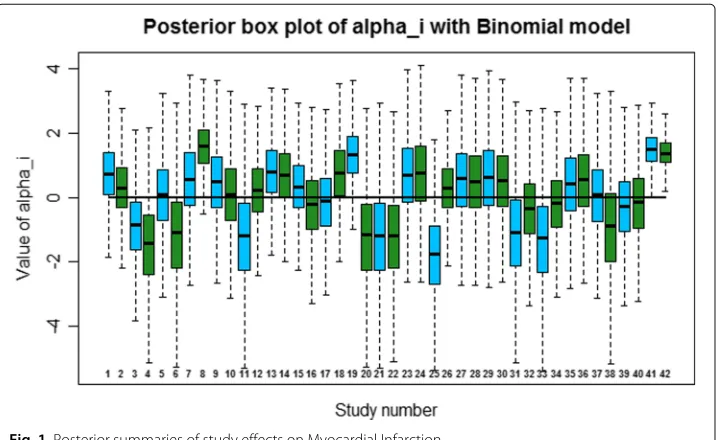
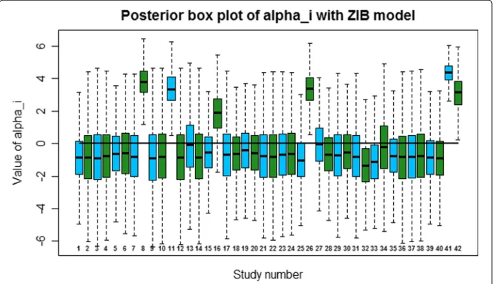
provide information on diabetes patients, 42 diabetes trials, and possible heart condition or death resulting from the use of rosiglitazone. Rosiglitazone is a treatment for diabetes widely used in treating patients with type 2 diabetes. We separately apply the model on myocardial infarction and death from cardiovascular based on these 42 studies. There were 86 myocardial infarctions in the rosiglitazone group and 72 in the control group. There were 39 deaths from cardiovascular causes in the rosiglitazone group and 22 in the control group. Note that the percentages of observed zeros from the 42 studies in the treatment and control arms for myocardial infarction are 23% and 57% respectively. Sim-ilar percentages for cardiovascular causes are 50% and 80% respectively. We set the hyper parameters asa=b= c=d=1,σ_H2 =2,σ_Tr2 =2 andσ_e2=2. Note that the choice of these values result sufficiently diffuse priors in the range of logit scale of primary param-eters. We implement the models developed in Section2using R. The results are based on a MCMC simulation with a burn-in period of 1000 iterations followed by 30,000 iter-ations using thinning of 5. We use the data from the 42 studies, without stratifying them into small and large studies, as the purpose of the proposed work is an illustration of the method and not in in-depth analysis of the data by using different methods or by slicing and dicing the data. The posterior box plots of study effects under two models on myocar-dial infarction are given in Figs.1and2. The advantage of using DP prior is the flexibility and also the ability to cluster studies appropriately. The clustering is based on the values assigned to each study effects based on their posterior distributions, which are approxi-mated using MCMC. Those studies that share the same study effects will be considered to belong to the same group. Note that there were 5 clusters in myocardial infarction and 4 clusters in cardiovascular causes based on study effects. To evaluate the performance between Binomial and ZIB models, we use the LPML which is based on Conditional Pre-dictive Ordinates(CPO). A detailed discussion of the CPO statistic and its applications to model selection can be found in Geisser (1993) and Gelfand and Dey (1994). The LPML

is computed as

k

#

i=1

logp(yi|y−i) wherey−i denotes the observation vectorywith theith

Fig. 2Posterior summaries of study effects on Myocardial Infarction

observation deleted. The model with larger value of LPML is preferred. The estimates of μ,Trand the LPML values are given in Table1. The LPML prefers binomial model over the ZIB model and the two models estimate the parameterTrdifferently.

We now investigate the study effects on death from cardiovascular causes. The pos-terior box plots of study effects under two models on death from cardiovascular causes are given in Figs.3and4. The plots indicate that ZIB model is capable in capturing the heterogeneity of study effects. The estimates ofμ,Trand the LPML values are given in Table1. In this case, the LPML strongly prefers ZIB model over the binomial model. This is in agreement with the fact that there are large amount of excessive zeros on death from cardiovascular causes relative to myocardial infarction.

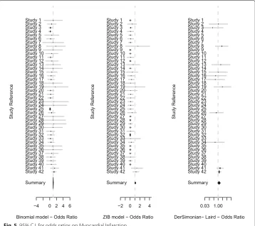
A summary of estimates of odds ratios under Binomial, zero inflated Binomial and DerSimonian- Laird random effects models are given in Figs.5and6. For myocardial infarction, DerSimonian- Laird random effects model gives an overall odds ratio of 1.29 with a 95% confidence interval of (0.9, 1.85). On the other hand, Binomial and zero inflated Binomial models provide an overall summary of odds ratio of 1.04 (0.98, 1.1) and 1.07 (0.97, 1.17) respectively. These estimates and 95% credible intervals for cardiovas-cular causes are 1.2 (0.64, 2.24), 1.03 (0.97, 1.09) and 1.13 (0.93, 1.33) respectively. It is clear that our approach provides overall odds ratios estimates that are slightly lower than that from DerSimonian- Laird overall estimate. Note that DerSimonian-Laird approach is based on the non-zero studies. Also note that Binomial and zero inflated Binomial mod-els identify more heterogeneous study effects than DerSimonian- Laird random effects

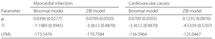
Table 1Parameter estimates with each model along with LPML

Myocardial infarction Cardiovascular causes

Parameter Binomial model ZIB model Binomial model ZIB model μ 0.0394 (0.0277) 0.0709 (0.0503) 0.0709 (0.0503) 0.1235 (0.0876) Tr -1.1989 (0.3945) -3.3612 (0.4870) -3.3612 (0.4870) -4.5339 (0.5707)

Fig. 3Posterior summaries of study effects on death from cardiovascular causes

model. According to Figs.5and6, we notice that zero inflated Binomial model identifies more heterogeneous effects than Binomial model while Binomial model identifies more heterogeneous effects than DerSimonian- Laird approach. DerSimonian- Laird estimated random effects variances are zero for both scenarios and this suggests that our approach is superier than DerSimonian- Laird random effects model when there is heteregeniety among studies and LPML model selection criteria will choose the best model in terms of prediction ability.

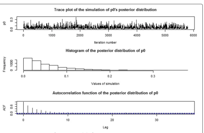
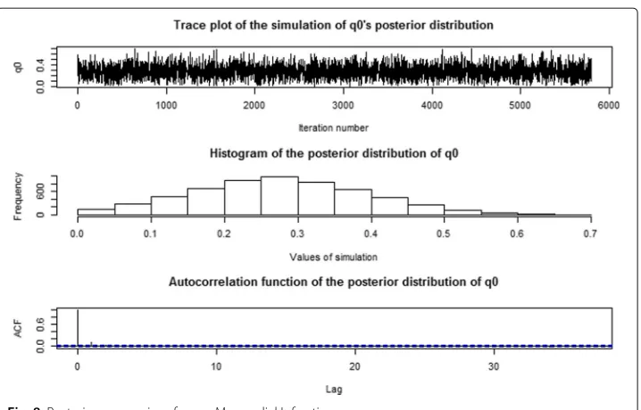
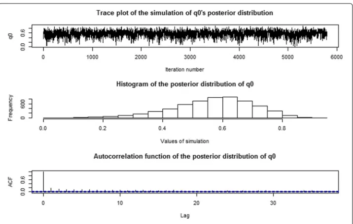
We now examine the effects of zero inflated parametersp0andq0on the analysis. The graphical posterior summaries ofp0andq0on myocardial infarction and cardiovascular causes are given in Figs.7,8,9and10. In addition, the numerical posterior summaries ofp0andq0are given in Table2. It is clear that the posterior distributions ofp0andq0

Fig. 595% C.I. for odds ratios on Myocardial Infarction

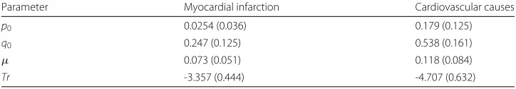
and their numerical summaries for myocardial infarction and cardiovascular causes make sense with respect to the percentages of zeros in the data. We also consider aBeta(0.5, 0.5) prior onp0andq0in order to investigate the prior sensitivity. The numerical posterior summaries ofp0andq0underBeta(0.5, 0.5)prior are given in Table3. We notice a magni-tude change in estimates ofp0andq0in this case but the estimates of primary parameters μandTrare very close indicating that odds ratios are not sensitive to the choice of prior settings. This indicates that inference onp0andq0will be sensitive to the choice of priors so one should select these priors carefully based on application specific apriori knowledge on zero inflated parameters.

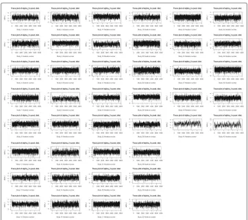
It is important to look at some convergence assessment plots related to the MCMC simulation as this is a high dimensional problem. The trace plot, histogram and autocor-relation plot ofμunder binomial model on Myocardial Infarction are given in Fig.11. The trace plot appears to stabilize immediately and hence provides no indication of lack of convergence in the Markov chain. The autocorrelation plot also appears to dampen quickly. Trace plots of study effects on Myocardial Infarction are given in Fig.12. The trace plots of study effects on death from cardiovascular causes indicate similar behavior. Similar plots were obtained for all of the parameters under each model and provide the evidence of the convergence of the Markov chains.

Note that one can also assign a simpler parametric normal prior on study effectsαiin

Fig. 695% C.I. for odds ratios on death from cardiovascular causes

Fig. 8Posterior summaries ofq0on Myocardial Infarction

DP prior in (2). In this case, forest plots of odds ratios for each model are given in Fig.13. The estimates of primary parameters of interest and LPML values are given in Table4. The LPML model selection criteria clearly indicates that the DP prior in (2) is superior than the conventional parametric prior.

Note that the overall decision to assess the safety should be based onp0,q0 and the overall odds ratio (OR). For example, the treatment can be declared is to be safer than the control, ifOR≤ 1, andp0 > q0. Also notice that estimates of(p0,q0)are independent of the odds ratio because the counts cannot be in “true" zero arms and “Binomial" arms. We combine the two metrics, conditional OR and(p0,q0), to come up with an overall

Fig. 10 Posterior summaries ofq0on cardiovascular causes

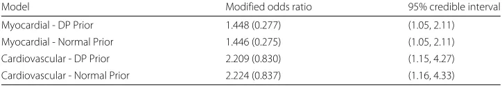
unconditional odds ratio. We define it to be modified odds ratio= OR×(1−p0)/(1−q0). Note that whenp0 = q0, modified odds ratio is same as OR. Ifp0 > q0, this adjusts OR, by multiplying by a factor less than 1, and ifp0 < q0, it adjust OR by multiplying by a factor> 1. This factor,h(p0,q0) = (1−p0)/(1−q0)is the ratio of probabilities of observing Bernoulli counts in the two arms, and can be considered as odds for observing Bernoulli counts in the two arms. In frequentist setup,h(pˆ0,qˆ0)is independent ofμ, andˆ hence independent of conditional odds ratio. In fact,pˆ0andqˆ0converge top0andq0with probability 1, and henceh(pˆ0,qˆ0)also converge toh(p0,q0)with probability 1, as h is a continuous function (from Slutsky’s theorem). So, the estimated modified odds ratio is a consistent estimator for unconditional odds ratio defined asOR×(1−p0)/(1−q0). We provide the estimates of the modified odds ratio for various models in Table5. As estimate ofp0is less thanq0for both examples (Myocardial Infarction and cardiovascular causes), the modified OR values are higher than the corresponding OR values.

4 Results from simulation studies

To understand the role ofp0andq0in the model, different simulation studies were carried out. For this purpose, we generate random ZIB values with empirical binomial parame-ters. We first generate 42 pairs of independent binary, 0 and 1, variables from Bernoulli (p0) and Bernoulli (q0) wherep0andq0are from the set of values{(0.1, 0.1), ...,(0.9, 0.9)}. We then assign the true-zeros at the places with 1s, and generate binomial outcomes from

B(n¯T,PˆTi)and fromB(n¯C,PˆCi), wheren¯T,n¯C,PˆTiandPˆCiare empirical estimates. Then,

MCMC sampling scheme described in Section2was carried out usingRto obtain the

Table 2Posterior mean and standard deviation (in parentheses) ofp0andq0

Parameter Myocardial infarction Cardiovascular causes

p0 0.0495 (0.044) 0.231 (0.117)

Table 3Posterior mean and standard deviation (in parentheses) ofp0andq0underBeta(0.5, 0.5) prior distribution

Parameter Myocardial infarction Cardiovascular causes

p0 0.0254 (0.036) 0.179 (0.125)

q0 0.247 (0.125) 0.538 (0.161)

μ 0.073 (0.051) 0.118 (0.084)

Tr -3.357 (0.444) -4.707 (0.632)

posterior estimate ofp0andq0. This was done 1000 times for each pair to obtain the mean and standard error of each estimate. For various scenarios of excessive zeros, the results are given in Table6. The results indicate that when true values ofp0is small and the observed values of zeros in the simulated data in treatment arm (control arm) is also small (large), the estimated values ofp0andq0are also small (large), whereas when the values ofp0andq0are large the simulated data has large proportion of zeros in both the arms, this results in large estimated values ofp0andq0. In both the situations, the esti-mated values ofp0andq0are in conformity with the observed percentages of zeros in the simulated data. The estimates ofp0andq0remain high in spite of their true choices from the parameter values. Note that our primary interest is on alphas and on treatment arm not on the control arm, so we may not need to investigate q0 very well as it can be trated as nuisance parameter. In practice, one should have a very good apriori knowledge of q0 which will allow to assign an informative prior as it is reflecting the zeros in the control arm. This indicates that the use of ZIB is more appropriate when there are excessive zeros in the data.

5 Discussion

Binary data naturally arise in clinical trials in health sciences. In some cases, they arise with excessive zeros. In this paper, we have provided a random effects meta analysis

Fig. 12 Trace plots of some study effects on Myocardial Infarction under binomial model

approach for binary data with excessive zeros in two-arm trials. The suitability of the bino-mial and zero inflated binobino-mial model was assessed in the presence of Dirichlet process as the prior for the study effects. The approach can be used as a template for meta analysis of binary data and a user may choose the proper model using log pseudo marginal like-lihood. We have shown that our approach is superior than DerSimonian- Laird random

Table 4Parameter estimates for various models underN0,σ_H2prior on study effects

Model μ Tr LPML Overall odds ratio with 95% C.I.

Myocardial - Bin 0.039 (0.028) -1.148 (0.369) -179.5883 1.04 (0.979, 1.101) Myocardial - ZIB 0.073 (0.052) -3.311 (0.435) -182.5765 1.07 (0.961, 1.194) Cardiovascular - Bin 0.036 (0.025) -1.892 (0.427) -161.3744 1.04 (0.983, 1.094)

Cardiovascular - ZIB 0.123 (0.089) -4.585 (0.568) -125.5402 1.13 (0.917, 1.356)

effects model when there is heterogeneity among studies and LPML model selection cri-teria can be used to selection the best model among the Bayesian models (not including DerSimonian-Laird model) for a given data set.

The Bayesian approaches discussed in this paper allowed to incorporate the zero-studies in the likelihood, and we found that the point estimates of the overall odds-ratio from these methods, were lower than the estimates reported in the literature Nissen and Wolski (2007). The use of ZIB model was to identify the percentage of excessive zeros, that is, the studies where the events could not occur, from the (Binomially) modeled zeros where the zero events occurred. Note that under ZIB, some zeros are observed with prob-abilityp0and some from Binomial model, making the probability of zero-event to be

p0+(1−p0)(1−PT)nT in the treatment arm. With the use of ZIB model, the Bayes

estimates of the odds-ratio went slightly up than with the use of Binomial model, but still they were lower than the results from DerSimonian-Laird random effects model and the resulting estimates in Nissen and Wolski (2007). Note also that DP model being dis-crete with probability 1, has a clustering property, where the study effects, that are alike, fall in the same cluster. We also investigated the suitability of the DP prior over the con-ventional parametric normal prior on study effects. The LPML model selection indicated that DP prior is superior than the conventional parametric normal prior. Finally, as the results from ZIB model on the parametersp0,q0and OR need to be interpreted together, a modified OR was introduced.

As a future direction of research, we would like to extend the approach discussed in this article for ordinal category data. For example, in some applications, the clinical trial end point could be a response variable in an ordinal scale with multiple categories such as Good/Moderate/Critical etc. This type of ordinal response data can be viewed as multivariate responses arising from continuous latent variables with cut-points. We assume that there is a continuous latent outcome behind these ordinal outcomes such thatXi = (Xi1,. . .,Xim) ∼ Normal(μ,)whereX’s are the latent outcomes andmis

the number of ordinal categories. Then the latent variablesXij’s can be converted to the

observedYijusing a cut-point vectorλ. However the choice of cut-points and their priors

need to be carefully selected as there are two arms and the counts on categories could be

Table 5Modified odds ratios, standard deviations (in parentheses) and credible intervals under DP and normal priors

Model Modified odds ratio 95% credible interval

Myocardial - DP Prior 1.448 (0.277) (1.05, 2.11)

Myocardial - Normal Prior 1.446 (0.275) (1.05, 2.11)

Cardiovascular - DP Prior 2.209 (0.830) (1.15, 4.27)

Table 6Simulation studies for the myocardial infarction data

Initial pair₍p0,q0) Mean of the

pos-terior means ofp0

estimates

Standard error of p0estimates

Mean of the pos-terior means ofq0

estimates

Standard error of q0estimates

(0.1,0.1) 0.19888206 0.0907763 0.52069774 0.08299897

(0.2,0.2) 0.29206103 0.10530334 0.59059405 0.05131143

(0.3,0.3) 0.33836514 0.09115085 0.62706227 0.06062431

(0.4,0.4) 0.3587838 0.10839263 0.63652 0.06102938

(0.5,0.5) 0.4977337 0.1267577 0.7200964 0.04900527

(0.6,0.6) 0.6180761 0.1255134 0.7705962 0.06610487

(0.7,0.7) 0.6525938 0.1885614 0.8096615 0.07434429

(0.8,0.8) 0.796206 0.09240875 0.8696273 0.06536744

(0.9,0.9) 0.8958989 0.0501579 0.935196 0.03310256

sparse. In this case, one can consider an objective Bayes approach following the develop-ment in Bayarri et al. (2008). Yet another extension of the proposed model is where there are multinomial data with some particular cell(s) being observed excessively. This kind of data may arise from trials with patient reported outcomes.

Acknowledgments

The authors thank Editor-in-Chief and three anonymous reviewers whose comments helped to improve the manuscript. This article reflects the views of the authors and should not be attributed to FDA’s views or policies.

Authors’ contributions

All authors have contributed equally to the work and approved the final version of the paper.

Funding

Muthukumarana’s research has been partially supported by a Discovery grant from the Natural Sciences and Engineering Research Council of Canada. Martell’s research internship was funded by Mitacs Globalink program.

Availability of data and materials

Data and code can be requested by contacting the authors.

Competing interests

The authors declare that they have no competing interests.

Author details

1_{Department of Statistics, University of Manitoba, Machray Hall, Winnipeg, Canada.}2_{ITAM, Mexico City, Mexico.}3_{Office of}

Biostatistics, Center for Drug Evaluation and Research, Food and Drug Administration, 10903 New Hampshire Ave,Silver Spring, USA.

Received: 13 September 2018 Accepted: 2 July 2019

References

Albert, J.: Teaching Inference about Proportions Using Bayes and Discrete Models. J. Stat. Educ.3(1995).https://doi.org/ 10.1080/10691898.1995.11910494

Bayarri, M. J., Berger, J. O., Datta, G. S.: Objective Bayes testing of Poisson versus inflated poisson models. Inst. Math. Stat.3, 105–121 (2008)

Branscum, A. J., Hanson, T. E.: Bayesian nonparametric meta-analysis using Polya tree mixture models. Biometrics.64, 825–833 (2008)

Burr, D., Doss, H.: A Bayesian semiparametric model for random-effects meta-analysis. J. Am. Stat. Assoc.100, 242–251 (2005)

Carlin, J. B.: Meta-analysis for 2×2 tables: A bayesian approach. Stat. Med.11, 141–158 (1992)

Chang, B. H., Waternaux, C., Lipsitz, S.: Meta-analysis of binary data: which within study variance estimate to use? Stat. Med.20, 1947–1956 (2001)

DerSimonian, R., Laird, N.: Meta-analysis in clinical trials. Control. Clin. Trials.7, 177–188 (1986) Ferguson, T. S.: Prior distributions on spaces of probability measures. Ann. Stat.2, 615–629 (1974)

Gamalo, M., Wu, R., Tiwari, R.: Bayesian approach to noninferiority trials for proportions. J. Biopharm. Stat.21, 902–919 (2011)

Geisser, S.: Predictive Inference: An Introduction. Chapman and Hall, London (1993)

Gelfand, A. E., Dey, D. K., Chang, H.: Model determination using predictive distributions with implementation via sampling-based methods (with discussion).Bayesian Statistics 4(Bernardo, J. M., Berger, J. O., Dawid, A. P., Smith, A. F. M., eds.) Oxford University Press (1992)

Ghosh, S. K., Mukhopadhyay, P., Lu, J. C.: Bayesian analysis of zero-inflated regression models. J. Stat. Plan. Infer.136(4), 1360–1375 (2006)

Hall, D. B.: Zero-Inflated Poisson and Binomial Regression with Random Effects: A Case Study. Biometrics.56, 1030–1039 (2000)

Huang, L., Zheng, D., Zalkikar, J., Tiwari, R.: Zero-inflated Poisson model based likelihood ratio test for drug safety signal detection. Stat. Methods Med. Res. (2014).https://doi.org/10.1177/0962280214549590

Muthukumarana, S., Tiwari, R.: Meta-analysis using dirichlet process. Stat. Methods Med. Res.25(1), 352–365 (2016) Neal, RM: Markov Chain Sampling Methods for Dirichlet Process Mixture Models. J. Comput. Graph. Stat.9(2), 249–265

(2000)

Nissen, S. E., Wolski, K.: Effect of rosiglitazone on the risk of myocardial infarction and death from cardiovascular causes. New Eng. J. Med.356, 2457–2471 (2007)

Smith, T. C., Spiegelhalter, D. J., Thomas, A.: Bayesian approaches to random-effects meta-analysis: a comparative study. Stat. Med.14, 2685–2699 (1995)

Publisher’s Note