A new efficient active contour model without local initializations for salient object detection

(1)

R E S E A R C H

Open Access

A new efficient active contour model without

local initializations for salient object detection

Riadh Ksantini

*

, Boubakeur Boufama and Sara Memar

Abstract

In this paper, we propose a fast and effective polarity-based active contour for salient object detection in grey-level images and color images. The adopted variational level set formulation forces the level set function to be close to a signed distance function and therefore completely eliminates the need of the re-initialization procedure and speeds up the curve evolution. Moreover, instead of the classical and widely used gradient-based stopping function, depending on the image gradient, to stop the curve evolution, we use a polarity-based stopping function. In fact, comparatively to the gradient information, the polarity information accurately distinguishes the boundaries or edges of the salient objects in images. One other nice result of the use of polarity information is that thead hocmanual and local initializations of the evolving curves inside and outside the image objects can be avoided. Therefore, one trivial and global initialization of the evolving curve can be performed to detect image salient objects. We also investigate the multi-spectral polarity information to generalize the proposed active contour to color images. Experiments are performed on several grey-level images and color images to show the advantage and the effectiveness of our new active contour model.

Keywords: Active contour model; Variational level set approach; Salient object detection; Multi-spectral gradient; Multi-spectral polarity; Color images

1 Introduction

In the last decades, image segmentation has been the subject of active research in computer vision and image processing. A large body of work on geometric active con-tours, i.e., active contours implemented via level set meth-ods, has been proposed to address a wide range of image segmentation problems [1-3]. Level set methods were first introduced by Osher and Sethian [4] for capturing mov-ing fronts. Active contours were introduced by Kass et al. [5] to segment objects in images using dynamic curves. The existing active contour models can be classified as either parametric active contour models or geometric active contour models according to their representation and implementation. In particular, the parametric active contours [5,6] are represented explicitly as parameterized curves in a Lagrangian framework, while the geomet-ric active contours [1,3,7] are represented implicitly as level sets of a two-dimensional function that evolves in an Eulerian framework. Geometric active contours were

*Correspondence: [email protected]

School of Computer Science, University of Windsor, ON N9B 3P4, Windsor, Canada

introduced by Caselles et al. [1] and Malladi et al. [3], respectively. These models are based on curve evolution theory [8] and level set method [9]. The basic idea is to evolve a level set function representing the contours according to a partial differential equation (PDE). The main advantage of this approach over the traditional para-metric active contours is that the contours represented by the level set function may break or merge naturally dur-ing the evolution, and the topological changes are thus automatically handled [10]. Early geometric active con-tour models [1,3,7] utilize a Lagrangian formulation that leads to a certain evolution PDE of a parametrized curve. Then, a new evolution PDE for a level set function is obtained using the related Eulerian formulation from level set methods. More precisely, the new evolution PDE can be directly derived from the problem of minimizing a certain energy functional defined on the level set func-tion. These methods are known as variational level set methods [11-13]. These methods are more robust than the pure PDE-driven level set methods. In fact, they are more convenient for incorporating additional information

(2)

such as shape and region location [14]. In implement-ing the traditional level set methods, it is numerically necessary to keep the evolving level set function close to a signed distance function [9,15]. Re-initialization, a technique for periodically re-initializing the level set func-tion to a signed distance funcfunc-tion during the evolufunc-tion, has been extensively used as a numerical remedy for maintaining stable curve evolution and ensuring usable results. However, re-initialization can cause a disagree-ment between the theory of the level set method and its implementation [16]. Moreover, it has a disadvantageous side effect of moving the zero level set away from its origi-nal location. Generally speaking, the problem is when and how to apply the re-initialization [16]. For this reason, Chunming et al. [17] proposed a new variational formu-lation that forces the level set function to be close to a signed distance function and therefore completely elim-inates the need of the costly re-initialization procedure. The variational level set formulation presented in [17] has three main advantages over the traditional level set for-mulations. First, a significantly larger time step can be used for numerically solving the evolution PDE and there-fore speeds up the curve evolution. Second, the level set function could be initialized as functions that are com-putationally more efficient to generate than the signed distance function. Third, the proposed level set evolution can be implemented using simple finite difference scheme, instead of complex upwind scheme as in traditional level set formulations [17]. However, like most of classical snakes and active contour models, the model proposed in [17] relies on edge indicator functions or gradient-based stopping functions, depending on the image gradient, to stop the curve evolution. These models can detect only objects with edges defined by gradient. In practice, the discrete gradient modules can have relatively small local maximums on the object edges and then the stopping function can be relatively far from zero on the edges, and the curve may pass through the boundary. Also, the local maximums of the discrete gradient modules in the tex-tured or noisy regions can be very close or equal to those of the object edges. Therefore, the evolving curve may stop before reaching the object boundaries. Moreover, if the image is very noisy, the isotropic smoothing Gaussian (used to compute the gradient module values) has to be strong, which will smooth the edges too. To solve these problems, we propose a stopping function which is based on the polarity information of the image edges. The polar-ity vanishes or is very close to zero inside a noise or texture region, whereas it maintains values very close to 1 on the relevant or main region edges. Consequently, the evolv-ing curve will stop at these edges. Combinevolv-ing the polarity information with the active contour model of [17] has two advantages. First, thead hocmanual and local initializa-tions of the evolving curves inside and outside the image

objects can be avoided. Only one trivial and global initial-ization of the evolving curve can be performed to detect image salient objects. Second, we obtain a fast and re-initialization-free active contour model which is robust to the textured and noisy regions. We also investigate the multi-spectral polarity information to generalize the pro-posed active contour to color images. The computation of the multi-spectral polarity is based on the multi-spectral gradient proposed by [18].

1.1 Related work

(3)

acts like edge stopping function in GAC model, which stops the contour evolution on the object boundaries. Moreover, like C-V model, the proposed active con-tour model is able to automatically detect all concon-tours regardless of the location of the initial contour. Also, a Gaussian filter was applied to regularize level set func-tion and avoid re-initializafunc-tion. More recently, in [32], the authors proposed a novel reaction-diffusion method for implicit region-based active contours [33], which is completely free of the costly re-initialization procedure in level set evolution. This method outperforms other clas-sical region-based active contours methods, especially, on noisy images. Note that the active contour models in [32] and [30] were mainly conceived to deal with image with intensity inhomogeneity. However, region-based active contours generally suffer from low performance on images with high-intensity inhomogeneity, such as, texture [14].

Recently, active contour models, which exploit together region and boundary information, are proposed in the literature. We can mention Allili and Ziou [14] who pro-posed an unsupervised color-texture image segmentation method based on active contour. The variational level set formulation adopted relies on a stopping function which utilizes polarity information of the image edges. However, its active contour model is based on homo-geneous seed initialization for different image regions. Moreover, it does not avoid the costly re-initialization procedure, and its curve evolving process is based on an expectation-maximization type algorithm [34] to fit the mixture parameters to the region data enclosed by the contours after evolution, which is computationally expen-sive. More recently, Tian et al. [35] proposed a level set active contour combining edge and region information. Its level set formulation consists of the edge-related term, the region-based term, and the regularization term. The edge-related term is derived from the image gradient and facil-itates the contours evolving into object boundaries [7]. The region-based term is constructed using both local and global statistical information and related to the direction and velocity of the contour propagation [36]. The last term ensures stable evolution of the contours [37,38]. Finally, a Gaussian filtering is used to regularize the level set func-tion following each iterafunc-tion, which avoids the calculafunc-tion of a signed distance function and re-initialization. How-ever, in [35], the boundary information is also represented by the classical gradient.

This paper is organized as follows. In Section 2, we will explain the derivation of the polarity information, and we will compare it to the gradient information. Also, we will present the multi-spectral and grey-level gradient infor-mation and then explain the derivation the multi-spectral and grey-level polarity information. In Section 3, we will describe our new active contour model which is the com-bination of the active contour model of [17] with the

polarity information. Section 4 provides an experimen-tal evaluation and comparison of the polarity-based active contour to the edge-based active contour proposed in [17] and to the region-based active contour models proposed in [30] and [31], on grey level and color images. Finally, we present our conclusions.

2 The polarity information

The most common type of edge detection techniques has used gradient operators, of which there have been numer-ous variations [5,11-13,17,39]. To detect salient region or object borders, we employ the pixels’ polarity. Using polarity information, we can figure out whether a pixel lies on textured or noisy regions or on an edge separating two salient regions. In fact, comparatively to the gradient information, the polarity information accurately discrim-inates the boundaries of the salient objects. The pixel

(x,y) polarityP((x,y)) [14,34] is a local image property described as a measure of the extent to which the gra-dient vectors in a certain neighborhoodℵ((x,y))of(x,y) are oriented in the same and dominant direction that we denote by −→η. Thus, the method looks at the structure of the gradient vectors in the pixel (x,y) neighborhood ℵ((x,y)). This structure is represented by the following second-moment matrix (or structure matrix).

Mσ(x,y)=

(u,v)∈ℵ((x,y))

Gσ(u,v)(∇I(u,v))(∇I(u,v))T, (1)

where∇I(u,v)is the gradient of the image intensity at the pixel(u,v)in the neighborhoodℵ((x,y))of the pixel(x,y)

andGσ = √₂1_πσexp−

u2+v2

2σ2 _{is a smoothing Gaussian kernel}

with varianceσ2. The scaleσ is defined to be the width of the Gaussian window within which the gradient vec-tors of the image are pooled. Moreover, this smoothing scale should be adapted to the texture in hand since coarse textures need larger scale values than fine ones. Assume now thatm1andm2are the eigenvalues ofMσ(x,y), where

m1> m2. Asm1>>m2, the neighborhoodℵ((x,y))has

a dominant orientation in the direction of the eigenvector that corresponds tom1. This eigenvector represents−→η.

Therefore, we express the polarity informationP((x,y))at the pixel(x,y)by the following function:

P((x,y))=

(u,v)∈ℵ((x,y))

Gσ(u,v) ∇I(u,v), − →_η ∇I(u,v) −→η ,

=

(u,v)∈ℵ((x,y))

Gσ(u,v) ∇I(u,v) −

→_η _cos_(ς) ∇I(u,v) −→η ,

=

(u,v)∈ℵ((x,y))

(4)

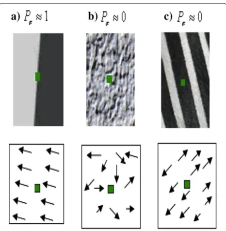
wheredenotes the vector scalar product andς repre-sents the angle between the vectors∇I(u,v)and−→η. The smoothing scale for the pixel(x,y)is chosen by looking at the behavior of the polarity to the changing of the value of the scaleσ. In a typical image region, homogeneous in color or texture, region edges will be located where the polarity maintains values near 1 for all possible scale val-ues (cos(ς = 0) =1 in sum (2)) (see Figure 1a); whereas, the polarity vanishes inside a homogeneous color inten-sity or texture regions as the value of the scale is increased (since multiple vector directionsςs will be included in the sum (2)) (see Figure 1b,c). By varying the scaleσ from 1 to 6, we choose the smoothing scale beyond which the polarity does not vary more than a fixed thresholdT.

For color or multi-spectral images, edges are typically modeled as color changes which are not only associated with color brightness discontinuities or color intensity contrast between the homogeneous regions but also with orientation changes of the color vectors associated to the color image pixels. According to [18], a color image edge detection is based on finding local maxima in the first directional derivative of the vector-valued color intensity function, which represents the color image and asso-ciates to each color image pixel a vector containing the local color channels. The magnitude of the strongest change of the vector-valued function which represents the multi-spectral gradient module coincides with the largest

Figure 1Different values of the polarity of a pixel represented by the green point.In a(a)salient boundary separating two different regions(P1),(b)noisy or texture region(P0), and(c) homogeneous color intensity region₍P0₎(The arrows represent the gradient vectors).

eigenvalue of the matrixJTJ, denoted byλmax, whereJis the Jacobian matrix of the vector-valued function repre-senting the color image. Thus, the multi-spectral gradient ∇I(u,v)at the pixel(u,v)in the neighborhood of(x,y)is simply the eigenvectorϑ( u,v)associated with the largest eigenvalueλmax(u,v)[18]. Note that gradient information in grey-level images is only a particular case of multi-spectral images. In this case, the image is represented by a single-valued color intensity function, and ∇I(u,v) =

∂I(u,v)

∂u ,

∂I(u,v)

∂v

is computed by the convolution of the image with the first derivative of a Gaussian filter along each dimension.

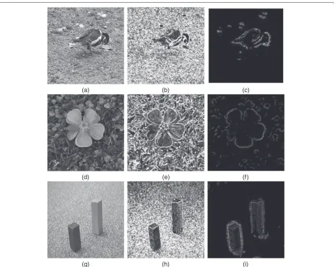
From Figure 2, we can clearly notice that compara-tively to the gradient information, the polarity information accurately distinguishes the boundaries or edges of the salient objects.

3 The active contour model using polarity information

In image segmentation, active contours are dynamic curves that moves toward the object boundaries. To achieve this goal, an external energy is defined to move the zero level curve toward the object boundaries. LetI be a grey-level image andgbe the classical gradient-based stopping function defined by

g=

₁

1+|∇I|2 ifIis a grey-level image, 1

1+λ2

max ifIis a multi-spectral image,

(3)

Most of the classical snakes and active contour models use this function as a stopping criteria [5,11-13,17]. The functiongis supposed to vanish when the active contour is very close to the boundaries. However, in practice, the discrete gradient modules |∇I| and λmax can have rela-tively small local maximums on the object edges and then the stopping function can be relatively far from zero on the edges, and the curve may pass through the boundary. Also, for the textured or noisy regions,|∇I|andλmaxcan be very close or equal to those of the object edges. There-fore, the evolving curve may stop before reaching the object boundaries. Moreover, if the image is very noisy, the isotropic smoothing Gaussian (used to compute the gra-dient module values) has to be strong, which will smooth the edges too. Hence, we propose the use of a stopping function based on the polarity information and defined by

gp=

1−P(I) polarityP(I)for grey-level imageI, 1−Pm(I) polarityPm(I)for multi-spectral imageI.

(4)

(5)

(a) (b) (c)

(d) (e) (f)

(g) (h) (i)

Figure 2Comparison between polarity information and gradient information.(a, d, g)Original grey-level images;(b, e, h)gradient images of the original images; and(c, f, i)polarity images of the original images (σ =6).

Combining the proposed polarity-based stopping func-tion with the variafunc-tional formulafunc-tion of [17], a total energy function can be defined as follow:

E(φ)=μ

1

2(|∇(φ)| −1)

2_dxdy

+λ

gpδ(φ)|∇φ|dxdy+ν

gpH(−φ)dxdy,

(5)

whereλ > 0 andνare constants,φis the level set func-tion [40],δ is the univariate Dirac function, ∈ 2, H is the Heaviside function, and the first term1₂(|δ(φ)− 1|2₎_dxdy_{is a metric or penalizing energy to characterize}

how close a functionφis to a signed distance function in

, this penalization is controlled by the parameterμ. The metric plays a key role in the variational level set formu-lation, since it avoids the costly re-initialization procedure while the active contour is evolving [17]. The total energy

E(φ)drives the zero level set toward the object bound-aries while penalizing the deviation of φ from a signed distance function during its evolution. The total energy function is minimized using calculus of variations [41] and the Gateaux derivative (first variation) of the functional E(φ)in Eq. (5). Since the functionφ that minimizes this functional satisfies the Euler-Lagrange equation ˛A∂_∂φE =0. The steepest descent process for minimization of the functionalEis the following gradient flow:

∂φ

∂t =μ[φ−div( ∇φ

|∇φ|)]+λδ(φ)div(gp_|∇∇φ_φ_|)+νgpδ(φ), (6)

(6)

need for the upwind scheme [10,17] as in the traditional level set methods. Instead, all the spatial partial derivatives

∂φ

∂x and∂φ∂y are approximated by the central difference, and the temporal partial derivative ∂φ_∂_t is approximated by the

forward difference [17]. So, the approximation in Eq. (6) can be simply written as

φk+1

i,j =φki,j+τL(φik,j), (7)

(7)

where τ is the time step. The coefficient ν can be pos-itive or negative, depending on the relative position of the initial contour to the object of interest. For exam-ple, if the initial contours are placed outside the object, the coefficient ν in the weighted area term should take

positive value so that the contours can shrink faster. If the initial contours are placed inside the object, the coefficientν should take negative value to speed up the expansion of the contours. However, since the stopping functiongp depends on the polarity information, thead

(8)

hocmanual and local initializations of the evolving curves inside the image objects can be avoided, as the noise and texture outside the objects have no more effect or removed.

4 Experimental results

In this section, in order to tease out the advantage of using polarity information, we compare the active con-tour model based on the polarity information to the

(9)

gradient-based active contour model of [17], on grey-level and color images, and to the region-based active con-tours proposed in [30] and [31], on only grey-level images. These comparisons are performed on 17 grey-level images (standard 256 color map images) and RGB color images, and the results are illustrated in Figures 3, 4, 5, and 6. From

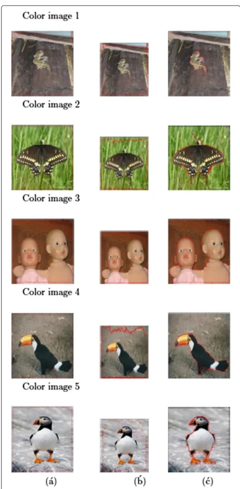
Figure 6Comparison between the two active contour models. (a)First column (left to right) - original color images with initial active contours (represented by red lines),(b)second column (left to right) -segmentation results using multi-spectral gradient-based active contour, and(c)third column (left to right) - segmentation results using multi-spectral polarity-based active contour.

these figures, we can clearly notice that the proposed active contour model based on the polarity information outperforms significantly the other active contour mod-els, on all the grey-level images and color images used, in term of salient object detection. Moreover, we can see that the salient objects in each image are efficiently detected using the polarity-based active contour, despite of the global and easy initialization of the evolving curve out-side of the salient objects. Hence, no more need for the ad hoclocal initializations of the evolving curves inside and outside the image objects. For example, to detect the desired object in Image 12 using the gradient informa-tion, the initialization of the evolving curve should be performed manually and locally inside the desired object. However, this latter can be easily detected using the polar-ity information and a global and simple initialization of the evolving curve, since the noise around the desired object is removed thanks to the polarity smoothing. Here, the proposed method outperforms the region-based active contour models, since the used images are clouted with texture and noise, and the region-based active con-tours generally show low performance in segmenting and detecting objects in images with high-intensity inhomogeneity.

In implementing the proposed level set method, the time stepτcan be chosen significantly larger than the time step used in the traditional level set methods [17]. We have tried several values of the time stepτ in our experiments for the different grey-level and multi-spectral images, ranging from 0.1 to 80. Also, according to our experi-ments, we have found that in order to maintain stable active contour evolution, the time stepτ and the coeffi-cientμmust be chosen such a way thatτμ <0.25. More-over, we noticed that using larger time stepτcan speed up the evolution but may cannot locate the boundary prop-erly, ifτ is chosen relatively too large. There is a tradeoff between choosing larger time step and accuracy in bound-ary location. Usually, we have used 5≤τ ≤10 for most of the grey-level and multi-spectral images. Generally speak-ing, for most of the grey-level and multi-spectral images, we used the parameters λ = 5, μ = 0.04, and ν = 3 (note that we should setν = −3 if the initial level set is computed from the region enclosed by the salient object), and the curves evolutions take from 280 to 600 iterations. Since most of the grey-level and multi-spectral images used in our experiment have coarse textures, the polar-ity smoothing scale was generally chosen relatively large

(10)

Table 1 Values of the objective criteria (OC) of our active contour model and the active contour models of [17,31] and [30], computed on grey-level images

Image OC withg([17]) OC with [31] OC with [30] OC withgp(ours)

Grey-level image 1 0.11 0.26 0.4 0.48

Grey-level image 2 0.15 0 0.55 0.65

Grey-level image 3 0.12 0.52 0.57 0.67

Grey-level image 4 0.1 0.4 0.35 0.45

Grey-level image 6 0.09 0.01 0.4 0.46

Grey-level image 8 0.18 0.04 0.49 0.56

Grey-level image 9 0.17 0.2 0.42 0.52

Grey-level image 10 0.2 0.47 0.18 0.57

Grey-level image 11 0.14 0.58 0.32 0.63

Grey-level image 12 0.09 0.47 0.42 0.54

active contour to stop evolving slightly (not remarkable for most of the images used in our experiments) before the ground truth edges, to end with a negligible edge localiza-tion error. Nevertheless, our segmentalocaliza-tion performance remains much more better than the other active con-tour models proposed in [17,30] and [31]. Note that with small or moderateσvalues for fine textures, we have bet-ter edge localization or localization property of polarity information.

In experimenting the method in [30], the initial con-tour was set globally, such a way, it includes all image objects. The experiments were conducted with different values of the variance (also denoted byσ) and with differ-ent numbers of iterations. More precisely, the number of iterations was set to 600 and the parameterσwas set to 7

for best results. Small values ofσ lead to the undesirable results, and large values make the experiment costly and very time-consuming.

In experimenting the method in [31], the initial contour was set globally, such a way, it includes all image objects. The numbers of iterations (range of values from 80 to 150) and the parameter denoted byα(range of values from 5 to 80) were set according the image used. Other parameters were kept fixed as default values for all images.

In order to compare and measure the segmentation accuracies of our active contour model and the models proposed in [17,31] and [30], we use the objective cri-terion proposed in [42] and the well-known Dice and Jaccard similarity measures. We first denote by Ri,i ∈ {1, 2, ...,NR}and R´j,j ∈ {1, 2, ...,NR´ } the sets of regions

Table 2 Values of the Jaccard (J) similarity of our active contour model and the active contour models of [17,31] and [30], computed on grey-level images

Image J withg([17]) J with [31] J with [30] J withgp(ours)

Grey-level image 1 0.15 0.17 0.45 0.51

Grey-level image 3 0.14 0.45 0.57 0.62

Grey-level image 4 0.12 0.41 0.32 0.48

Grey-level image 6 0.1 0.04 0.37 0.41

Grey-level image 8 0.2 0.03 0.46 0.51

Grey-level image 9 0.2 0.22 0.34 0.49

Grey-level image 10 0.25 0.46 0.15 0.59

Grey-level image 11 0.16 0.54 0.25 0.67

(11)

Table 3 Values of the Dice (D) similarity of our active contour model and the active contour models of [17,31] and [30], computed on grey-level images

Image D withg([17]) D with [31] D with [30] D withgp(ours)

Grey-level image 1 0.15 0.2 0.48 0.54

Grey-level image 3 0.15 0.51 0.59 0.66

Grey-level image 4 0.13 0.45 0.41 0.5

Grey-level image 6 0.12 0.06 0.4 0.45

Grey-level image 8 0.22 0.05 0.5 0.56

Grey-level image 9 0.25 0.27 0.43 0.54

Grey-level image 10 0.29 0.49 0.34 0.64

Grey-level image 11 0.17 0.61 0.32 0.7

Grey-level image 12 0.12 0.47 0.45 0.55

or segments composing the segmentation of a tested or evaluated active contour model and the ground truth (i.e., perfect segmentation of the silent objects), respectively. The objective criteria (OC) measures the accuracy error of boundary localization between segmented regions and ground truth regions. The objective criteria is zero for worst segmentation and is equal to one for perfect seg-mentation. The Dice and Jaccard similarities measure the overlap between the segmented regions and ground truth regions. They are defined as the size of the intersection of the segmented regions and ground truth regions divided by the size of their union. The Jaccard (J) and Dice (D) similarities are zero if the two regions are disjoint, i.e., they have no common pixels, and are equal to one if the regions are identical. Higher similarity values indicate better agreement in the regions. The Dice and Jaccard similari-ties facilitate the interpretation of the evaluation results in terms of the standard ‘False Positive,’ ‘False Negative,’and ‘True Positive’ ratios. In our case, the segmented regions represent the ‘False Positive,’ the ground truth regions rep-resent the ‘False Negative,’ and the intersection between the ground truth regions and segmented regions represent the ‘True Positive.’ A higher ‘True Positive’ relatively to

‘False Positive’ plus ‘False Negative’ corresponds to better matching between ground truth regions and segmented regions and then to better segmentation performance. In Tables 1, 2, and 3, we illustrate, respectively, the val-ues of the objective criterion and the Dice and Jaccard similarities computed on the grey-level images, using the compared active contour models. For the color images, the computed objective criterion and Dice and Jaccard similarities, using the polarity-based active contour and the gradient-based active contour, are shown in Table 4. From these tables, we can clearly notice that our active contour model yields the least error or the best accuracy of boundary localization comparatively to the models of [17,31] and [30], for all grey-level images and color images used.

5 Conclusions

We have proposed a fast and efficient active contour model for salient object detection in grey-level images and color images. By combining the polarity informa-tion with the active contour model of [17], the salient objects can be easily detected. In fact, comparatively

Table 4 Values of the objective criteria (OC), Jaccard (J), and Dice (D) of our active contour model and the active contour model of [17], computed on the multi-spectral images

Image OC withg OC withgp J withg J withgp D withg D withgp

Color image 1 0.08 0.68 0.12 0.71 0.13 0.75

Color image 2 0.11 0.65 0.15 0.7 0.16 0.74

Color image 3 0.15 0.71 0.18 0.75 0.2 0.8

Color image 4 0.13 0.69 0.16 0.73 0.17 0.77

(12)

to the gradient information, the polarity information accurately distinguishes the boundaries or edges of the salient objects. Moreover, thanks to the use of polarity information, thead hoclocal initializations of the evolv-ing curves inside and outside the image objects can be avoided, since the noise and texture outside the object have no more effect or removed. Our experimental results showed clearly that the proposed active contour model based on the polarity information outperforms signifi-cantly the gradient-based active contour model of [17] and the relevant region-based active contour models of [31] and [30], in terms of salient object detection and segmentation accuracy, especially, on real-world textured images with high-intensity inhomogeneity. Future work will be dedicated improve the performance of the pro-posed active contour using relevant region and shape information.

Competing interests

The authors declare that they have no competing interests.

Acknowledgements

We would like to thank Dr. Zhang Kaihua for providing us with the source code of the region-based active contour models proposed in [31] and [30]. This work was supported by the NSERC program and the University of Windsor.

Received: 8 September 2012 Accepted: 14 June 2013 Published: 18 July 2013

References

1. V Caselles, F Catte, T Coll, F Dibos, A geometric model for active contours in image processing. Numer. Math.66, 1–31 (1993)

2. X Han, C Xu, J Prince, A topology preserving level set method for geometric deformable models. IEEE Trans. Patt. Anal. Mach. Intell.25, 755–768 (2003)

3. R Malladi, JA Sethian, BC Vemuri, Shape modeling with front propagation: a level set approach. IEEE Trans. Patt. Anal. Mach. Intell.17, 158–175 (1995) 4. S Osher, JA Sethian, Fronts propagating with curvature dependent speed:

algorithms based on Hamilton-Jacobi formulations. J. Comp. Phys.79, 12–49 (1988)

5. M Kass, A Witkin, D Terzopoulos, Snakes: active contour models. Int. J. Comp. Vis.1, 321–331 (1987)

6. C Xu, J Prince, Snakes, shapes, and gradient vector flow. IEEE Trans. Imag. Proc.7, 359–369 (1998)

7. V Caselles, R Kimmel, G Sapiro, Geodesic active contours. Int. J. Comp. Vis. 22, 61–79 (1997)

8. BB Kimia, A Tannenbaum, S Zucker, Shapes, shocks, and deformations I: the components of two-dimensional shape and the reaction-diffusion space. Int. J. Comp. Vis.15, 189–224 (1995)

9. S Osher, R Fedkiw,Level set methods and dynamic implicit surfaces. (Springer-Verlag, New York, 2002)

10. JA Sethian,Level set methods and fast marching methods. (Cambridge University Press, Cambridge, 1999)

11. T Chan, L Vese, Active contours without edges. IEEE Trans. Imag. Proc.10, 266–277 (2001)

12. B Vemuri, Y Chen,Joint image registration and segmentation. (Geometric Level Set Methods in Imaging, Vision, and Graphics Springer, New York, 2003)

13. H Zhao, T Chan, B Merriman, S Osher, A variational level set approach to multiphase motion. J. Comp. Phys.127, 179–195 (1996)

14. MS Allili, D Ziou, Globally adaptive region information for automatic color-texture image segmentation. Pattern Recognit. Lett.28, 1946–1956 (2007)

15. D Peng, B Merriman, S Osher, H Zhao, M Kang, A PDE-based fast local level set method. J. Comp. Phys.155, 410–438 (1999)

16. J Gomes, O Faugeras, Reconciling distance functions and level sets. J. Visiual Communic. and Imag. Representation.11, 209–223 (2000) 17. C Li, C Xu, C Gui, MD Fox, Level set evolution without re-initialization:

a new variational formulation. Int. Conf. Comput. Vis. Pattern Recognit. 1, 430–436 (2005)

18. C Drewniok, Multispectral edge detection: some experiments on data from landsat-tm. Int. J. Remote Sens.15(18), 3743–3765 (1994) 19. A Kumar, P Olver, AJ Yezzi, S Kichenassamy, A Tannenbaum, A geometric

snake model for segmentation of medical imagery. IEEE Trans. Med. Imag. 16(2), 199–209 (1997)

20. LD Cohen, On active contour models and balloons. CVGIP:Image Understand.53(2), 211–218 (1991)

21. A Mitiche, A Mansoursi, C Vásquez, Multiregion competition: a level set extension of region competition to multiple region image partitioning. Comput. Vis. Image Understand.101(3), 137–150 (2006)

22. A Tsai, A Yezzi, AS Willsky, A fully global approach to image segmentation via couples curve evolution equations. J. Vis. Commun. Image Rep. 13(1-2), 195–216 (2002)

23. A Mitiche, I Ben Ayed, Z Belhadj, Multiregion level set partitioning on synthetic aperture radar images. IEEE Trans. Pattern Anal. Mach. Intell. 27(5), 793–800 (2005)

24. T Brox, M Rousson, R Deriche, Active unsupervised texture segmentation on a diffusion based feature space. IEEE Conf. Comput Vis. Pattern Recognit.2, 677–704 (2003)

25. C Garcia, E Sifakis, G Tziritas, Bayesian level sets for image segmentation. J. Vis. Commun. Image Rep.13(1), 44–64 (2002)

26. N Paragios, R Deriche, Geodesic active regions: a new paradigm to deal with frame partition problems in computer vision. J. Vis. Commun. Image

Rep.13(1-2), 249–268 (2002)

27. N Paragios, R Deriche, Geodesic active regions and level set methods for supervised texture segmentation. Int. J. Comput. Vis.46(3), 223–247 (2002) 28. BS Manjunath, R Chellappa, Unsupervised texture segmentation using

Markov random field models. IEEE Trans. Pattern Anal. Mach. Intell.13(5), 478–482 (1991)

29. J Puzicha, T Hofmann, JM Buhmann, Unsupervised texture segmentation in a deterministic annealing framework. IEEE Trans. Pattern Anal. Mach. Intell.20(8), 803–818 (1998)

30. K Zhang, H Song, L Zhang, Active contours driven by local image fitting energy. Pattern Recognit.43(4), 1199–1206 (2010)

31. K Zhang, L Zhang, H Song, W Zhou, Active contours with selective local or global segmentation: a new formulation and level set method. Image Vis. Comput.28(4), 668–676 (2010)

32. K Zhang, L Zhang, H Song, D Zhang, Re-initialization free level set evolution via reaction diffusion. IEEE Trans. Image Process.22(1), 258–271 (2013)

33. T Chan, L Vese, Active contours without edges. IEEE Trans. Image Process. 10(2), 266–277 (2001)

34. C Carson, S Belongie, H Greenspan, J Malik, Blobworld: Image segmentation using expectation-maximization and its application to image querying. IEEE Trans. Pattern Anal. Mach. Intell.8(24), 1026–1038 (2002)

35. M Zhou, Y Tian, F Duan, Z Wu, Active contour model combining region and edge information. Machine Vis. Appl.24(1), 47–61 (2011)

36. H Song, K Zhang, L Zhang, W Zhou, Active contours with selective local or global segmentation: a new formulation and level set method. Image Vis. Comput.28(4), 668–676 (2010)

37. JC Gore, C Li, C Kao, Z Ding, Minimization of regionscalable fitting energy for image segmentation. IEEE Trans. Image Process.17(10), 1940–1949 (2008)

38. JC Gore, C Li, C Kao, Z Ding, Implicit active contours driven by local binary fitting energy. IEEE Conf. Comput. Vis. Pattern Recognit.1, 1–7 (2007) 39. J Canny, A computational approach to edge detection. IEEE Trans. Patt.

(13)

40. VI Arnold,Geometrical methods in the theory of ordinary differential equations. (Springer-Verlag, New York, 1983)

41. L Evans,Partial differential equations. (American Mathematical Society, Providence, 1998)

42. D Martin, C Fowlkes, D Tal, J Malik, A database of human segmented natural Images and its application to evaluating segmentation algorithms and measuring ecological statistics. IEEE Int. Conf. Comput. Vis.2, 416–423 (2001)

doi:10.1186/1687-5281-2013-40

Cite this article as:Ksantiniet al.:A new efficient active contour model

without local initializations for salient object detection.EURASIP Journal on

Image and Video Processing20132013:40.