Understanding Type Ia Supernovae Through Their Host Galaxies Using the SDSS-II Supernova Survey

(1)

University of Pennsylvania

ScholarlyCommons

Publicly Accessible Penn Dissertations

1-1-2013

Understanding Type Ia Supernovae Through Their

Host Galaxies Using the SDSS-II Supernova

Survey

Ravi Ryan Gupta

University of Pennsylvania, [email protected]

Follow this and additional works at:http://repository.upenn.edu/edissertations

Part of theAstrophysics and Astronomy Commons, and thePhysics Commons

This paper is posted at ScholarlyCommons.http://repository.upenn.edu/edissertations/758

For more information, please [email protected].

Recommended Citation

Gupta, Ravi Ryan, "Understanding Type Ia Supernovae Through Their Host Galaxies Using the SDSS-II Supernova Survey" (2013).

Publicly Accessible Penn Dissertations. 758.

(2)

Understanding Type Ia Supernovae Through Their Host Galaxies Using

the SDSS-II Supernova Survey

Abstract

The recent discovery of the accelerating expansion of the Universe and thus the existence of dark energy was made possible by the study of Type Ia supernovae. These thermonuclear explosions of white dwarfs are excellent standardizable candles that can be seen out to great distances and used to constrain cosmological parameters. However, in an era when modern surveys are discovering hundreds of Type Ia supernovae and upcoming surveys plan to find thousands more, we are no longer limited by statistics, but are now being limited by systematic uncertainties in supernova cosmology. Among these systematic uncertainties are the nature of the supernova progenitor and the effect of the environment on the progenitor. An excellent way to probe these systematics is through the study of the galaxies that host Type Ia supernovae. Correlations have been found between supernova properties and the physical properties of their host galaxies such as mass, metallicity, and star formation rate. In this dissertation, I use supernovae from the full three-year Sloan Digital Sky Survey II (SDSS-II) Supernova Survey and multi-wavelength photometry of their host galaxies to find evidence of a correlation between supernova luminosities and the age of their hosts, a possible proxy for progenitor age. I also detail a method of host galaxy identification, tested and applied to the many thousands of SDSS-II supernova candidates, which will be published in the upcoming final data release of the Supernova Survey. In addition, I present work in which I compute the luminosity functions for Type Ia supernovae and their host galaxies. This work and continuing work in this vein can help shed light on the nature of dark energy and improve the utility of Type Ia supernovae as cosmological distance indicators.

Degree Type

Dissertation

Degree Name

Doctor of Philosophy (PhD)

Graduate Group

Physics & Astronomy

First Advisor

Masao Sako

Keywords

Galaxies, Observational Cosmology, Supernovae

Subject Categories

Astrophysics and Astronomy | Physics

(3)

UNDERSTANDING TYPE IA SUPERNOVAE THROUGH THEIR HOST

GALAXIES USING THE SDSS-II SUPERNOVA SURVEY

Ravi Ryan Gupta

A DISSERTATION

in

Physics and Astronomy

Presented to the Faculties of the University of Pennsylvania

in Partial Fulfillment of the Requirements for the Degree of Doctor of Philosophy

2013

Supervisor of Dissertation

Masao Sako, Associate Professor of Physics and Astronomy

Graduate Group Chairperson

A. T. Charlie Johnson, Professor of Physics and Astronomy

Dissertation Committee

James Aguirre, Assistant Professor of Physics and Astronomy

Mariangela Bernardi, Associate Professor of Physics and Astronomy

Adam Lidz, Assistant Professor of Physics and Astronomy

(4)

Dedication

For Mom and Pop, who made many sacrifices to open as many doors for

me as possible, and who encouraged me to pursue my interests, whatever

they may be. From them I learned the importance of education, working

hard, and trying my best, no matter what. And for my girlfriend, Kelly,

who has been a constant source of support, care, and love despite being

3810.4 kilometers away.

(5)

Acknowledgments

First, I would like to begin by thanking my advisor, Masao Sako, whose teachings,

guid-ance, and mentorship are not limited to my time here at Penn. As an undergraduate at

Stanford, I had the privilege of working with Masao, who was a postdoctoral research

fellow there at the time. From him I have learned early on the basic tools necessary to

do research, from Unix computing and shell scripting to data analysis and thinking like a

scientist.

I am also indebted to my officemates and colleagues who, over the years, have become

good friends. They have always taken the time to teach or better explain things to me,

and I have learned an incredible amount from them all. Therefore, thanks to fellow Sako

Group members Chris D’Andrea, Jennifer Mosher, John Fischer, and Rachel Cane with

whom I’ve discussed many supernova-related and computer-related issues over the years.

Thanks also to C. Jonathan MacDonald for his programming insights, and to Mariangela

Bernardi, Ravi Sheth, and Alan Meert, whose expertise in the field of galaxies has been

invaluable. My years here at Penn have been some of the most enjoyable of my life. For

this I must thank, in addition to those previously mentioned, Annemarie Exarhos, Phil

Korngut, Josh Kunkle, Andrés Plazas, and Liz Hines.

I have benefited greatly from being a part of the Sloan Digital Sky Survey II Supernova

Survey and the Dark Energy Survey Supernova Survey. In particular, I would like to thank

John Marriner of Fermilab and Richard Kessler of the University of Chicago for their help

and guidance in several key aspects of research presented in this dissertation.

(6)

Additionally, I would like to acknowledge my grade school teachers Robin Dickerson,

Steve Gouger, Reg Hendrickson, and Joseph Vanderway for their part in piquing my

interest in the sciences. I would also like to thank Duane Doty of the California State

University, Northridge who helped me solve the “chicken or the egg” research dilemma by

giving me a chance and allowing me to work with him even though, as a college freshman,

I had no prior research experience. During my later college years, I was thankful to

have the opportunity to get a head start on astrophysics research under the supervision of

Steven Kahn at Stanford University and his postdoctoral researchers at the time: Masao,

John Peterson, and Ming Feng Gu.

Finally, I thank my committee members James Aguirre, Mariangela Bernardi, Adam

Lidz, and Elliot Lipeles for their help and patience.

(7)

ABSTRACT

UNDERSTANDING TYPE IA SUPERNOVAE THROUGH THEIR HOST GALAXIES

USING THE SDSS-II SUPERNOVA SURVEY

Ravi Ryan Gupta

Masao Sako

The recent discovery of the accelerating expansion of the Universe and thus the existence

of dark energy was made possible by the study of Type Ia supernovae. These

thermonu-clear explosions of white dwarfs are excellent standardizable candles that can be seen out

to great distances and used to constrain cosmological parameters. However, in an era

when modern surveys are discovering hundreds of Type Ia supernovae and upcoming

sur-veys plan to find thousands more, we are no longer limited by statistics, but are now being

limited by systematic uncertainties in supernova cosmology. Among these systematic

un-certainties are the nature of the supernova progenitor and the effect of the environment on

the progenitor. An excellent way to probe these systematics is through the study of the

galaxies that host Type Ia supernovae. Correlations have been found between supernova

properties and the physical properties of their host galaxies such as mass, metallicity, and

star formation rate. In this dissertation, I use supernovae from the full three-year Sloan

Digital Sky Survey II (SDSS-II) Supernova Survey and multi-wavelength photometry of

their host galaxies to find evidence of a correlation between supernova luminosities and

the age of their hosts, a possible proxy for progenitor age. I also detail a method of host

galaxy identification, tested and applied to the many thousands of SDSS-II supernova

candidates, which will be published in the upcoming final data release of the Supernova

Survey. In addition, I present work in which I compute the luminosity functions for Type

Ia supernovae and their host galaxies. This work and continuing work in this vein can

help shed light on the nature of dark energy and improve the utility of Type Ia supernovae

as cosmological distance indicators.

(8)

List of Tables

2.1 FSPS model grid parameters . . . 34

3.1 Host matching statistics for SDSS SN candidates . . . 57

4.1 SN Ia sample selection summary . . . 70

4.2 Hostless SNe Ia . . . 74

4.3 SN Ia fit results for the LF,x1, andcdistributions . . . 84

4.4 SN Ia host galaxy Schechter fit results . . . 91

4.5 SN Ia host galaxy double Gaussian fit results . . . 91

A.1 Properties of SN Ia Sample and Host Galaxies . . . 105

(11)

List of Figures

1.1 The width-luminosity & color-luminosity relations . . . 9

1.2 Combined results of the SCP and the HZT . . . 12

1.3 Redshift distribution of SDSS spectroscopic SNe Ia . . . 15

1.4 SDSS-II 1st year Hubble diagram . . . 16

1.5 Effect of progenitor metallicity on the width-luminosity relation . . . 20

1.6 Hubble residual vs. host mass for nearby SNe Ia . . . 22

1.7 Hubble residual vs. host mass from SNLS and SDSS . . . 23

2.1 GALEX, SDSS, and UKIDSS filter response curves . . . 31

2.2 Host mass uncertainty vs. redshift . . . 36

2.3 Distributions of host age and age uncertainty . . . 37

2.4 Host age vs. mass . . . 38

2.5 SN stretch vs. host age . . . 39

2.6 SN color vs. host age . . . 40

2.7 Hubble residual vs. host age . . . 42

2.8 Hubble residual vs. host mass . . . 43

2.9 Hubble residual vs. host age and mass for the “control” samples . . . 46

3.1 Diagram illustrating the host matching technique . . . 50

3.2 Distribution of the truth sample as a function ofdDLR . . . 53

3.3 Efficiency, purity, and figure of merit of the host-matching algorithm . . . 54

3.4 Distribution of SN candidate-host separation . . . 56

3.5 Observed and simulated host galaxym_r distributions . . . 58

3.6 Distribution of SN Ia host galaxies in the mass-SFR plane . . . 62

3.7 Distributions of SN Ia host galaxy mass, age, and SFR . . . 64

4.1 Maximum apparentr-band mag of SN vs. redshift . . . 71

4.2 Redshift distribution of the base and magnitude-limited samples . . . 72

4.3 Redshift distribution comparison of simulations to data . . . 76

4.4 Luminosity function of SNe Ia . . . 82

4.5 Distribution of SALT2x1andc . . . 83

4.6 SN Ia LFs split by redshift and host galaxy type . . . 85

4.7 Distribution of SALT2x₁andcsplit by host galaxy type . . . 86

4.8 Luminosity function of host galaxies in thegband . . . 88

(12)

4.9 Luminosity function of host galaxies in therband . . . 89

4.10 Luminosity function of host galaxies in theiband . . . 90

4.11 Host galaxy LF in therband split by host galaxy type . . . 92

4.12 Simulated SN Ia rate errors . . . 95

(13)

Chapter 1 Introduction

1.1 Cosmology and the Expanding Universe

Within the past fifteen years, we have unexpectedly discovered not only that the

expan-sion of the Universe is accelerating, but also that the agent responsible accounts for nearly

70% of the mass-energy of the Universe. This component has been dubbed “dark energy.”

Modern field theories are unable to produce a compelling explanation for dark energy,

and so it remains one of the greatest unsolved problems in physics today. Its existence

was discovered through observations of Type Ia supernovae (SNe Ia) (Riess et al. 1998;

Perlmutter et al. 1999), and though it has been confirmed through independent

measure-ments, SNe Ia are currently the most mature and precise method for studying dark energy

through distance measurements (Howell 2011). While most researchers agree that the

progenitor of a SN Ia is a carbon-oxygen white dwarf residing in a binary star system,

all are uncertain about the exact nature of the binary companion and the details of the

explosion physics (Whelan & Iben 1973; Nomoto et al. 1984; Hillebrandt & Niemeyer

2000). Therefore, investigations of SNe Ia are crucial for determining the nature and

ori-gin of dark energy and understanding the expansion history and future of the Universe.

In this section, I review the relevant aspects of cosmology and explain why the surprising

discovery of dark energy has caused us to change our view of the cosmos.

(14)

1.1.1 Expansion History

When Edwin Hubble first plotted the velocity of galaxies as a function of their distance,

he found that these galaxies are receding and that their velocities increase linearly with

their distances (Hubble 1929). From this first “Hubble diagram” came the revelation that

the Universe is expanding, and that the velocityvof galaxies is related to their distanced

by

v=H₀d, (1.1)

whereH0 is theHubble constant, traditionally measured in units of km s−1 Mpc−1. In

fact, H₀ is the present-day value of the more fundamental quantity called the Hubble

parameter,H(t). Hubble’s linear relationship above is valid to first order for small

veloc-ities, but in modern times, measurements of recessional velocity have been abandoned in

favor of the redshift. The wavelength of light emitted from a receding source,λ_emitted, is

effectively stretched to longer wavelengths so that the wavelength we observe,λ_observed,

is redder. This is known as the redshift,z, and is defined as

1+z_≡ λobserved

λ_emitted . (1.2)

In addition, it is useful to define an arbitrary length scale in the Universe called the

scale factor,a, which is a function of cosmic time. Cosmologists seta=1 today whilea

takes smaller values at earlier times. The scale factor is related to the redshift via

1+z= 1

a, (1.3)

and related to the Hubble parameter via

H(t)_≡a˙

a, (1.4)

where ˙adenotes the derivative ofawith respect to time. Equation 1.4 is useful as it tells

us how rapidlyachanges and thus how rapidly the Universe is expanding.

Constructing Hubble diagrams (i.e., plotting the distance-redshift relation) by means

of measuring the redshift and distance of faraway objects tells us about the evolution of

(15)

energy density in the Universe and puts constraints on cosmological parameters, as we

will see later on. Measuring the redshift simply requires obtaining a spectrum of the

distant source and identifying absorption or emission features, but measuring distances in

astronomy is much more difficult since the night sky is a two-dimensional projection of

the visible Universe and the intrinsic size and brightness of celestial objects is often not

known. The observed fluxF from an object with luminosityLis

F = L

4πD2_L,

(1.5)

whereDLis called theluminosity distance. Thus, if the luminosity of an object is known,

measuring the flux will yield the luminosity distance. Objects whose L is known are

referred to as standard candles, and as explained in Section 1.2, SNe Ia happen to be such

objects and as a result are very useful for cosmology.

1.1.2 Magnitudes and Distance Moduli

Historically, astronomy (at least around the optical portion of the electromagnetic

spec-trum) uses magnitudes rather than flux to measure brightness. The magnitude system

dates back to the time of the ancient Greek astronomer Hipparchos who ranked stars

based on a six magnitude system, with the brightest being first magnitude and those that

are barely visible being sixth magnitude (Ryden 2003). The magnitude system was then

formalized by Sir Norman Pogson, who defined them to be logarithmic (Pogson 1856).

In defense of Hipparchos and Pogson, the human eye does perceive brightness roughly

logarithmically, although it is better described by a power law (Schulman & Cox 1997).

Owing to these reasons, the Pogson magnitude system, though counterintuitive, is still

used in astronomy today. Theapparent magnitude mof an object is defined by the

loga-rithm of the ratio of the observed flux f of the object to some standard flux f₀.

m=−2.5 log

f f₀

. (1.6)

(16)

It is also convenient to define the absolute magnitude M of an object as the apparent

magnitude an object would have if it were a distance of 10 parsecs (pc) away.

M=−2.5 log

L

f₀_×4π(10 pc)2

. (1.7)

Just asmis a measure of the flux or apparent brightness of an object,Mis a measure of

its luminosity or intrinsic brightness.

Thedistance modulus µ is then defined as the difference between the apparent and

absolute magnitudes.

µ ≡m₋M=5 logDL−5, (1.8)

whereD_Lis measured in pc. In this form,µ can be thought of as a measure of distance in

units of magnitudes. This is a somewhat theoretical expression for the distance modulus

sinceD_L depends not only on the redshift (a direct observable) but also on cosmological

parameters, which are not directly measurable. Actual observations are made from Earth

with instruments that collect light through sets of filters. Therefore, in practice we must

also correct the apparent magnitude for Milky Way extinction andK-correction. Milky

Way extinction is simply the Galactic reddening along the line of sight due to the

absorp-tion and scattering of light in interstellar space. TheK-correction is a term that must be

added to account for the fact that a distant object that is observed in some filter must be

converted to an equivalent measurement in the restframe of the object in order for a direct

comparison to be made betweenmandM. This is dependent on the redshift and spectral

energy distribution (SED) of the object and also on the filter response functions of the

instrument performing the observations. Extinction and K-correction are denoted by A

andK, respectively, and these corrections are implicitly assumed to be included in min

writing Equation 1.8. In order to be explicit, we write the full expression wherem_obs is

the apparent magnitude as measured by the observer.

(m_obs₋A₋K)−M=5 logD_L₋5. (1.9)

Note that prior knowledge of the intrinsic luminosity and the SED of the object (or at least

some assumption about them) is needed to obtainMandK. Thus, from Equation 1.9, we

(17)

can determineD_L (or equivalently,µ from Equation 1.8) to effectively estimate distances

and test cosmology. In SN cosmology Hubble diagrams are often plotted as µ versusz.

The slope at low-redshift from SNe in the local Universe constrainsH₀but higher redshift

SNe are necessary to then determine evolution inH.

1.1.3 A Census of the Universe

The Universe consists of several components: matter (mostly dark matter), radiation, and

the newest addition, dark energy1. The mass densities of these are denoted by ρi, and

each component can be treated as a fluid with its own equation of state:

P_i=w_iρic2, (1.10)

wherePi is the pressure, cis the speed of light, andwiis known as the equation of state

parameter. Assuming w_iis constant for each component, p_i evolves with the expansion

of the Universe as

ρi(z) =ρi,0(1+z)3(1+wi), (1.11)

whereρi,0denotes the current density. Ifwi>−1, the component dilutes with expansion,

and such is the case for non-relativistic matter and radiation. It is the evolution of the

expansion rate,H(z), that puts contraints on these components in the framework of

Ein-stein’s theory of general relativity (GR). Cosmologists often work with the dimensionless

density parameterΩi=ρi/ρc, where ρc is known as the critical density and is the total

density necessary for a spatially flat Universe. Let us use the subscripts M, R, k, and

DE to denote matter, radiation, curvature, and dark energy, respectively. From GR and

Friedmann’s dynamical equations for a homogeneous and isotropic Universe, H(z) can

be related to the components of the Universe by

H2(z) =H₀2

h

ΩM,0(1+z)3+ΩR,0(1+z)4+Ωk,0(1+z)2+ΩDE,0(1+z)3(1+wDE)

i

.

(1.12)

1_{Spatial curvature can also be treated as a component mathematically.}

(18)

The radiation term can be ignored since at the present time, ΩR,0 .10−4 (Astier

2012; Ryden 2003). Theory and observational evidence indicates that the Universe is

very close to spatially flat (Guth 1981; de Bernardis et al. 2000; Komatsu et al. 2011;

Planck Collaboration XVI 2013), so often the Ωk,0 term is assumed to be zero. Note

that current observations from SNe alone and also combined with other measurements

such as cosmic microwave background (CMB) and baryon acoustic oscillations (BAO)

are consistent withw_DE =−1 (Conley et al. 2011; Sullivan et al. 2011), in which case the

dark energy term is independent of redshift. This form of dark energy is referred to as the

cosmological constant, Λ. Also, it is possible for wDE to vary with time, in which case

theΩDE,0term in Equation 1.12 becomes more complicated. Prior to 1998, cosmologists

believed that our Universe was matter-dominated and so after the initial expansion from

its original dense state (the so-called Big Bang), the expansion should continually slow

due to the mutual gravitational attraction of matter. However, observations of SNe Ia

showed that this was not the case.

1.2 Type Ia Supernovae

Type Ia supernovae (SNe Ia) are a key measurement in determining the standard

cos-mological model. Their distance calibration based on empirical relations between SN Ia

peak luminosity and both light-curve width and optical colors (Phillips 1993; Hamuy et al.

1996b; Riess et al. 1996) provides evidence for the accelerated expansion of the Universe

and the existence of dark energy (Riess et al. 1998; Perlmutter et al. 1999). Historically,

absolute distances to SNe Ia at low redshift were calibrated to extragalactic supergiant

stars known as Cepheid variables whose luminosities are correlated with their pulsation

period. However, with peak luminosities of_∼1036 W (_∼100,000 times more luminous

than Cepheids) (Howell 2011; Ryden 2003), SNe Ia are favored for cosmology since they

can be seen out to greater distances and can probe high redshifts where the

distance-redshift relation is nonlinear (e.g., see bottom left panel of Figure 1.2 for a comparison

(19)

of how varying cosmologies affect values of the distance modulus). After correcting for

light-curve shape and color, SNe Ia can provideDL measurements with precision better

than 6% (0.12 mag) (Perlmutter & Schmidt 2003; Weinberg et al. 2012).

1.2.1 Classification and Progenitors

Supernovae were originally classified according to features in their spectra and the shapes

of their light curves (brightness as a function of time). Those classified as Type Ia contain

no hydrogen in their spectra, but do contain strong absorption from ionized silicon (SiII)

(da Silva 1993). We now believe SNe Ia are thermonuclear explosions and therefore differ

fundamentally from other types of SNe which are caused by gravitational core-collapse

of young massive stars (M_&8M) (Smartt 2009). Although the progenitor of a SN Ia

has never been directly observed, the consensus is that it is a carbon-oxygen (CO) white

dwarf (WD) that gains mass from a binary companion. At some point, the WD approaches

the Chandrasekhar mass ofM_Ch_≈1.38M (Chandrasekhar 1931) and carbon is ignited,

triggering an explosion that unbinds the WD. The thermonuclear fusion of C and O in

the WD progenitor produces intermediate mass elements (Mg, Si, S, Ca) along with

iron-peak elements (Ni, Co, Fe) (Hillebrandt & Niemeyer 2000). The light curve is powered

by the Comptonization of γ-rays produced by the radioactive decay of 56Ni (t1_/₂=6.1

days)_→56Co (t1_/₂=77 days)→56Fe, where t1_/₂indicates the half-life of decay (Colgate

& McKee 1969; Stritzinger et al. 2006; Astier 2012).

In order to reproduce observations, models have shown that that the flame must start

subsonically (deflagration) and eventually become supersonic (detonation) (Khokhlov

1991; Kasen et al. 2009), although the physics of the explosion are still not completely

understood. Also unknown is the exact nature of the progenitor system(s). Two main

models exist: the single-degenerate (SD) and the double-degenerate (DD). In the SD

sce-nario, the companion is a non-degenerate star such as a main sequence or red giant that

donates mass to the WD via Roche lobe overflow or a stellar wind (Whelan & Iben 1973).

In the DD scenario, the companion is another WD and the two degenerate stars spiral in

(20)

as a result of energy loss from gravitational radiation and eventually coalesce (Iben &

Tu-tukov 1984; Webbink 1984). SNe Ia might be formed from either one of these channels

or possibly a mixture of the two.

1.2.2 Standardizable Candles

Even due to possible differences in progenitor and explosion scenarios, SNe Ia are

re-markably standard candles, with a room mean square (rms) dispersion of_≈0.4 mag in

peakV-band luminosity (Hamuy et al. 1996a; Riess et al. 1996)2. Phillips (1993) found

the decline rates of SNe Ia are tightly correlated with their peak brightnesses in the sense

that SNe Ia with slower declining light curves are also intrinsically brighter. This is

of-ten referred to as the Phillips relation, width-luminosity relation, or the brighter-slower

relation. In addition, a relationship with SN color exists (albeit weaker than the

width-luminosity relation) such that bluer SNe are brighter and redder ones are dimmer (Riess

et al. 1996; Tripp 1998). This is usually referred to as the color-luminosity relation or the

brighter-bluer relation.

Kasen & Woosley (2007) suggest that overall, the width-luminosity relation is due to

line-blanketing by numerous FeII/CoII lines. This causes dimmer (and thus generally

cooler) SNe Ia to experience an earlier onset of recombination which results in a more

rapid evolution of SN colors towards the red. Therefore, faster ionization evolution of

iron group elements is responsible for fasterB-band decline rates in dimmer SNe. While

the cause of the full diversity of SNe Ia is not completely known, it is known that

empiri-cally correcting for the width and color relations greatly improves distance measurements.

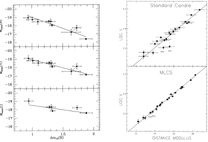
A plot from Phillips (1993) (left panel) and another from Riess et al. (1996) (right panel)

illustrate this improvement and are reproduced in Figure 1.1. The left panel demonstrates

the existence of the width-luminosity relation where the width of the light curve is

param-eterized by∆m15(B), which is the B-band magnitude decrease from the time of peak to

15 days later. The upper plot of the right panel shows the scatter in the Hubble diagram

2_{However, extreme cases of SNe Ia can vary by a factor of 10 in peak luminosity (Phillips 1993).}

(21)

1993ApJ...413L.105P

No. 1, 1996 TYPE Ia SN MULTICOLOR LIGHT-CURVE SHAPES 105

FIG. 6.ÈHubble diagrams for SN IaÏs with velocities in theCOBErest frame on the Cepheid distance scale (Sandage et al.1994, 1996).All velocity errors

are 300 km s~1, reÑecting a plausible estimate of random velocities with respect to the Hubble Ñow. (a) Distances estimated with a standard luminosity assumption and no correction for extinction. This method yieldsp_v\0.52andH_{0 \}52^8(statistical) km s~1Mpc~1. (b) Distances from the MLCS method, which makes a correction for intrinsic luminosity variation and total extinction as determined from the light and color curve shapes. This method yieldsp_v\0.12andH_{0 \}64^3(statistical) km s~1Mpc~1.

suggest that the MLCS method provides remarkably precise, extinction-corrected distances that are a signiÐcant improve-ment over SN Ia distances from previous methods.

7.DISCUSSION

Our intent has been to describe the MLCS method in enough detail so others can take advantage of the precise distance estimates it provides. The strength of MLCS lies in its ability to disentangle the e†ects of absorption and intrinsic luminosity variations while providing meaningful error estimates. These measures are derived from the distance-independent observables of multicolor light-curve shapes. The accuracy of the MLCSrelativedistance measures has been well established on an independent set of 20 SN IaÏs on the Hubble diagram.

Figure 1.1 The width-luminosity & color-luminosity relations. LEFT: The

width-luminosity relation reproduced from Phillips (1993). The width of the light curve is

parameterized by∆m15(B)(B-band magnitude decrease from the time of peak to 15 days

later). SNe with broader light curves decline slower (i.e., have smaller values of∆m15(B))

and are intrinsically brighter.RIGHT: Hubble diagrams (velocity vs.µ) reproduced from

Riess et al. (1996) showing the reduction in scatter when correcting for intrinsic luminos-ity variation and extinction as determined from width and color. Even the subluminous SN 1992K and the highly-reddened SN 1995E (labeled) are corrected for by this method.

when SNe Ia are assumed to be standard candles (without corrections). The bottom plot

of the right panel corrects the SNe for stretch and color which greatly reduces the scatter.

In order to carry out a SN survey for the purpose of obtaining distance estimates, one

needs light curves with which to measure the decline rate and observations in multiple

filters with which to measure color. Generally, a set of empirical models are needed

to fit the observed data. Two of the most popular models currently used are the

Multi-color Light Curve Shape method (MLCS2k2; Jha et al. 2007) and the Spectral Adaptive

Lightcurve Template method (SALT2; Guy et al. 2007).

(22)

MLCS2k2 is photometry-based and works with a set of model light curves in the

standard visibleU BV RI bands, and observations must be K-corrected into these bands

before fitting. A single parameter called the “luminosity correction,”∆, is used to account

for the variation in observed light curves. MLCS2k2 trains on low-z events at known

distances and therefore outputs aµ value when fitting. The fitter has the option to use an

extinction prior, i.e., an assumption that the extinction of the ensemble follows a known

distribution, and it claims to be able to statistically separate color variations due to dust

from intrinsic SN color differences. After accounting for color variations that correlate

with light curve shape, it is assumed that the excess color is attributable to dust extinction

that follows the Milky Way extinction law. For each SN, the fitter outputs a value ofµ,∆,

aV-band extinction valueA_V, and a reference date.

SALT2 is a flux-based fitter and works by manipulating template SEDs and thusK

-corrections are trivial. By modifying a spectral time series it attempts to reproduce the

photometry of the training spectra and light curves. SALT2 does not assume anything

about the source of color variations, and models them by multiplying the SED flux by a

wavelength-dependent exponential extinction factor. The outputs of SALT2 are the date

ofB-band maximum, peakB-band apparent magnitudem_B(essentially the normalization),

a stretch parameter x1, and a color c. It does not return a µ value which allows

high-redshift SNe to be included in the training set. However, this means that another code,

such as SALT2mu (Marriner et al. 2011) is needed after SALT2 is run to obtainµ values.

From the output of SALT2, distances can be estimated from the linear relation

µ =mB−M+αx1−βc. (1.13)

where M (the SN absolute magnitude), α, and β are global parameters fit to the data

sample by minimizing the residuals in the Hubble diagram. SALT2mu is able to calculate

α and β independent of cosmology by minimizing the scatter in the Hubble relation in

small redshift bins.

All standardization methods rely heavily on empirical relations and assumptions. For

example, it is assumed that SNe Ia at low-zare representative of higher-zevents. Also, as

(23)

we shall see in Section 1.4, properties of the host galaxies have been found to correlate

with SN properties, and such correlations are not currently accounted for in the

stan-dardization process. Many uncertainties exist as well, such as SN color and host galaxy

extinction, and its treatment remains a point of contention. Further discussion of the

sys-tematic uncertainties that currently limit SN Ia cosmology is presented in Section 1.4.3.

1.2.3 Evidence for Acceleration

By the 1990s, modern digital instrumentation made the accurate detection of distant

ob-jects possible. In the middle of that decade, the Supernova Cosmology Project (SCP)

and the High-Z Supernova Search Team (HZT) began observing high-redshift SNe Ia

in an effort to measure the deceleration parameter, q₀, which is a function of the

den-sity parameters of the components of the Universe (Section 1.1.3). The value of q0 is

positive for a decelerating Universe. At the time, it was believed that the Universe was

matter-dominated and that mutual gravitational attraction was slowing the expansion rate,

and therefore q₀ >0 was the expected result. Both teams used SNe from the nearby

Calán/Tololo Supernova Search (CTSS; Hamuy et al. 1993) to anchor their measurements

and were granted time on large telescopes including theHubble Space Telescope (HST)

and the Keck Telescopes in order to obtain follow-up spectra of their high-redshift SNe.

Astonishingly, both teams found that high-zSNe were fainter than expected, indicating

q0<0 and anaccelerating Universe, contrary to expectations based on a Universe

con-taining mostly matter. Their discovery that the Universe was accelerating rather than

decelerating, as previously thought, garnered Saul Perlmutter (SCP), Brian Schmidt and

Adam Reiss (HZT) the 2011 Nobel Prize in Physics.

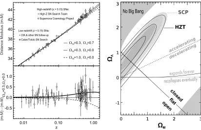
Figure 1.2 shows the combined results from the two heavily-cited papers by the SCP

(Perlmutter et al. 1999) and the HZT (Riess et al. 1998). The simplest solution to explain

this acceleration is to introduce a new component withw<₋1/3, the most common being

w=−1 (the cosmological constant, Λ) (Perlmutter & Schmidt 2003). Hubble diagrams

(24)

Measuring Cosmology with Supernovae 211

Fig. 4.Upper panel:The Hubble diagram for high redshift SNIa from both theHZSNS [83] and theSCP[77].Lower panel:The residual of the distances relative to aΩM= 0.3,

ΩΛ= 0.7 Universe. Thez <0.15 objects for both teams are drawn fromCTSSsample [32], so many of these objects are in common between the analyses of the two teams.

with aw < −0.5 is acceptable [23,77]. Additionally, we can add information about the value ofΩM, as supplied by recent 2dF redshift survey results [98], as shown in the 2nd panel, where the constraint strengthens tow <−0.6 at 95% confidence [69].

6 The Future

How far can we push the SN measurements? Finding more and more SNe allows us to beat down statistical errors to arbitrarily small levels but, ultimately, systematic eﬀects will limit the precision to which SNIa magnitudes can be applied to measure distances. Our best estimate is that it will be possible to control systematic eﬀects from ground-based experiments to a level of∼ 0.03

No Big Bang

1 2

0 1 2 3

expands forever -1 0 1 2 3 2 3 closed open recollapses eventually flat

M

decelerating accelerating HZT SCP

Figure 1.2 Combined results of the SCP and the HZT, reproduced and adapted from

Perl-mutter & Schmidt (2003). LEFT: The top panel shows the Hubble diagram anchored

by low-zsamples with 3 different cosmologies overplotted. The bottom panel shows the

residual plot relative to a ΩM =0.3, ΩΛ =0.0 cosmology. The data favors a non-zero

cosmological constant. RIGHT: Constraints from SNe Ia on the(ΩM,ΩΛ) plane where

the contours are the 1, 2, and 3σ confidence intervals. The data are consistent with a flat

Universe withΩM ≈0.3 andΩΛ≈0.0.

in the left panel show that a Universe with present-day densities3ofΩM =0.3,ΩΛ=0.7

are favored by the data over cosmological models withΩΛ=0. The right panel shows the

confidence contours for values ofΩM andΩΛ for both groups. Furthermore, assuming a

flat Universe, both teams found the significance ofΩΛ>0 to be roughly 3σand ruled out

a matter-dominated Universe at 7σ (Astier 2012).

These pioneering studies illustrated the true power of SNe Ia to constrain

cosmol-ogy. After the standardization process,µ values can be derived for each SN from

Equa-tion 1.13. Theseµ values are related toDL via Equation 1.8. And for a flat Universe with

only matter and dark energy (ΩM+ΩDE =1),DL is related to cosmological parameters

3_{The ",0" subscripts are often dropped so e.g.,}

ΩM,0becomes simplyΩM.

(25)

by

D_L= c

H₀(1+z)

Z

z

0

dz0

p

ΩM(1+z0)3+ΩDE(1+z0)3(1+w)

, (1.14)

wherewis the equation of state parameter of dark energy. Thus, from SNe Ia

measure-ments one can place constraints on cosmological parameters. The prevailing

cosmolog-ical model is a flat Universe containing approximately 5% baryonic matter (the matter

with which we are familiar), 27% cold dark matter, and 68% dark energy (of the formΛ)

(Planck Collaboration XVI 2013). This is known as a flat,Λ-Cold Dark Matter (ΛCDM)

cosmology. It is perhaps more than a bit troubling then that _≈95% of the Universe is

“dark” and composed of constituents of unknown nature.

1.3 Supernovae in the Sloan Digital Sky Survey

The Sloan Digital Sky Survey (SDSS)4 began as the brainchild of Princeton astronomer

Jim Gunn, and the collaboration has since expanded to include 25 institutions around the

world. In 2000, SDSS began collecting data and it continues to do so to this day, with the

latest data release being Data Release 9 (Ahn et al. 2012). The survey uses a large-format

wide-field charge-coupled device (CCD) camera mounted on a 2.5 m Ritchey-Chrétien

telescope located at Apache Point Obsevatory in New Mexico (Gunn et al. 1998, 2006).

SDSS is one of the largest and most successful photometric and spectroscopic surveys

ever conducted. The imaging array uses five filters,ugriz, that span the optical range from

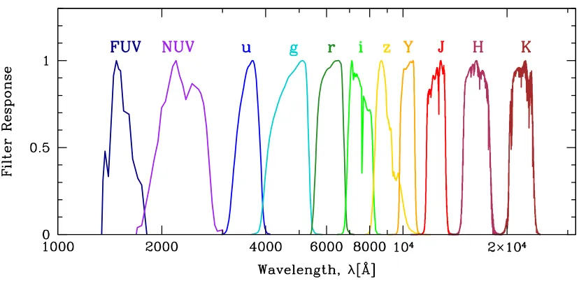
about 3000 Å to 11,000 Å (Fukugita et al. 1996; see also Figure 2.1). The photometric

survey takes advantage of the Earth’s rotation by using the technique known as

drift-scanning to efficiently image the sky in strips.

In 2005, SDSS began its second phase of operations which included the Sloan Digital

Sky Survey II Supernova Survey (SDSS-II SN Survey). The aim of the SN Survey was to

perform a rolling search by repeatedly scanning a 300 deg2equatorial strip of sky known

as Stripe 82 located approximately between 20 and 4 hours of right ascension (20h_.α.

4_{http://www.sdss.org/}

(26)

4h) and between₋1.25 and+1.25 degrees in declination (₋1.25◦_.δ.+1.25◦). During

the months of September through November from 2005 to 2007, the SDSS-II SN Survey

discovered SNe with a sampling cadence of five days on average, with each observation

obtaining 55-s integrated exposures in each filter. For point sources, SDSS achieved 50%

detection completeness atr=22.6; the typical peak magnitude for a SN Ia atz=0.2 is

r_≈20.8 (Frieman et al. 2008).

After standard SDSS processing, SN images are run through a difference imaging

pipeline where template frames are subtracted from search frames containing potential

transients. Then object detection and filtering algorithms are applied (Sako et al. 2008).

From this, light curves are constructed using the photometric technique dubbed “scene

modeling,” and the fluxes are calibrated to the Ivezi´c et al. (2007) standard star catalog

to obtain photometry accurate to_∼2% (Holtzman et al. 2008). Objects that passed

qual-ity cuts and were inspected by humans were then selected as targets for spectroscopic

follow-up. Spectroscopic facilities for this endeavor included the 2.4 m Hiltner telescope

at MDM, the 3.5 m Astronomy Research Consortium (ARC) telescope at Apache Point

Observatory (APO), the 9.2 m Hobby-Eberly Telescope (HET) at McDonald

Observa-tory, the 4.2 m William Herschel Telescope (WHT), the 8.2 m Subaru, the 10 m Keck I

telescope, the ESO New Technology Telescope (NTT) and the Nordic Optical Telescope

(NOT) (Zheng et al. 2008; Östman et al. 2011). The reduction, redshift measurement,

and classification of the spectra from the first season are described in Zheng et al. (2008),

while the NTT and NOT spectra taken in 2006-2007 are described in Östman et al. (2011).

The Subaru spectra taken in 2005-2006 are described in Konishi et al. (2011).

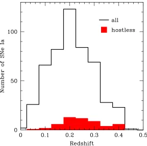
Over the three-year course of the SN Survey, 504 SNe were spectroscopically

con-firmed to be Type Ia. The redshift distribution of these SNe Ia is shown in Figure 1.3,

with the subset of “hostless” SNe (i.e., SNe whose host galaxies were too faint to be

detected by SDSS) shown in solid red. (Host galaxy identification is discussed in

Sec-tion 3.2.) These SNe lie in the redshift range 0.01_.z_.0.46 with a median redshift of

z_≈0.2. This intermediate range made SDSS unique at the time, since existing surveys

(27)

Figure 1.3 Redshift distribution of the 504 spectroscopically confirmed SNe Ia from the full three-year SDSS-II SN Survey. The full sample is shown in black and the subsample for which the corresponding hosts were too faint to be detected by SDSS (“hostless”) are shown in solid red.

either targeted nearby galaxies or were deep pencil-beam surveys optimized for high-z

events (Sako et al. 2008).

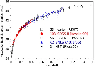
Figure 1.4 is the Hubble diagram adapted from the first-year SDSS-II SN Survey

cosmological analysis paper by Kessler et al. (2009a). The diagram shows the redshift

range probed by SDSS compared to other surveys and illustrates how it was crucial in

tying together the low-zand high-zevents. Using SN measurements fit with both SALT2

and MLCS2k2 combined with CMB and BAO data, Kessler et al. (2009a) found that a

conservative estimate ofwlies in the range₋1.1<w<−0.7. For both the SALT2 and

MLCS2k2 methods, the paper details an exhaustive analysis of systematic errors. They

attribute the SALT2-MLCS2k2 discrepancy to the rest-frameU-band in the SN models

(28)

34 36 38 40 42 44 46

0 0.2 0.4 0.6 0.8 1 1.2 1.4 1.6

ML C S 2k 2 fit te d di st an ce m od ul us (m ag )

33 nearby (JRK07)

103 SDSS-II (Kessler09)

56 ESSENCE (WV07) 62 SNLS (Astier06) 34 HST (Riess07)

redshift

Figure 1.4 Hubble diagram adapted from Kessler et al. (2009a) for the 288 SNe Ia from the five samples indicated on the plot. Note the unique redshift range probed by SDSS-II and that this plot contains SDSS-II data from 2005 only. A cosmological analysis using the full three-year sample is forthcoming.

and to the different treatment of color variations. They also comment that current SN Ia

samples have reached the systematic limits of light-curve fitters.

The abundance and richness of the SDSS-II SN Survey data have resulted in a plethora

of published papers. Studies of SNe Ia rates have been undertaken by Dilday et al. (2008,

2010) and Smith et al. (2012). Correlations between SNe Ia properties and properties of

their host galaxies (the main thrust of this thesis) have been found (Lampeitl et al. 2010;

Nordin et al. 2011; Gupta et al. 2011; D’Andrea et al. 2011; Galbany et al. 2012; Hayden

et al. 2013). Most recently, Campbell et al. (2013) published a cosmological analysis

using photometrically-classified SNe Ia. A full three-year data release paper (Sako et al.

2013, in prep.) and a complete three-year cosmology analysis are forthcoming.

(29)

1.4 Type Ia Supernova–Host Galaxy Correlations

1.4.1 Environmental Dependencies on SN Luminosities

In addition to the width-luminosity and color-luminosity relations that are used to

stan-dardize SNe Ia, researchers have found that SNe Ia properties can depend on environment.

Hamuy et al. (1995) found that galaxies with younger stellar populations (bluer color)

ap-pear to host the intrinsically brightest SNe Ia. A follow-up study (Hamuy et al. 1996a)

used a finer grid of galaxy types (E, S0, Sa, Sb, Sc, Irr) to strengthen the previous result

and found an even more interesting relationship between ∆m15(B) and morphological

type: spirals produce slow-declining SNe with a large spread in ∆m15(B)while

ellipti-cal galaxies produce only fast-decliners. Other authors also confirmed these observations

that SNe Ia in passively-evolving, elliptical galaxies are intrinsically fainter (Riess et al.

1999; Hamuy et al. 2000; Sullivan et al. 2006). Sullivan et al. (2010) note that though

light-curve correction should account for this effect, the cosmic star formation rate is a

function of redshift, and so these differences imply a shift in mean SN Ia properties.

Fur-thermore, in terms of star formation per unit stellar mass, SNe Ia are more than 10 times

more common in late-type, star-forming galaxies than in early-type, passively evolving

galaxies (Mannucci et al. 2005; Sullivan et al. 2006).

The origin of the differences in SN properties between spiral and elliptical galaxies is

currently unknown, though some believe they are due to fundamentally different

popula-tions of SNe Ia progenitors (Sullivan et al. 2006). Progenitor age or metallicity could also

be a factor in explaining these differences. Gallagher et al. (2005) analyzed the spectra of

57 local SN Ia host galaxies and found a correlation such that spiral galaxies with higher

metallicity host fainter SNe, though the result was not statistically significant. However,

they did find qualitative evidence to suggest progenitor age, rather than metallicity, is

the source of variability in SN luminosities. Restricting the analysis to early-type host

galaxies, Gallagher et al. (2008) used absorption-line spectra to compute the

luminosity-weight ages and metallicities for 29 hosts. They found a strong correlation indicating

(30)

that galaxies older than 5 Gyr host SNe Ia that are_∼1 mag fainter atV-band peak than

SNe in younger populations. They also found that metallicity has a weaker effect on SN

luminosity, although they note that even spectral analyses suffer from the age-metallicity

degeneracy introduced through the use of stellar population synthesis models.

1.4.2 Correlations with Hubble Residuals

After correcting SNe Ia for light curve shape and color, the scatter that remains in the

Hubble diagram around the best-fit cosmology is known as the Hubble residual (HR).

That is, for each SN Ia the HR is the difference between the value of the distance modulus

obtained from the SN (µSN) and the value obtained from the best-fit cosmology at the

redshift of the SN (µz). If HR scatter is truly random, then the fact that the age, metallicity,

mass, etc. of galaxies evolves with redshift ought not to bias cosmological measurements

using SNe Ia. However, if HR is found to correlate with one of these properties, this would

pose a problem for cosmology. As it so happens, such correlations have been discovered

in recent years.

Gallagher et al. (2005) observed a only a “tenuous” correlation between HR and host

metallicity. However, in their subsequent analysis using 17 early-type hosts (Gallagher et

al. 2008), such a correlation was seen at 98% confidence for a one-sided test. The trend

was such that metal-poor systems tend to produce underluminous SNe Ia after

correc-tion5. The study also found a negligible significance of a correlation between HR and

age. Hicken et al. (2009b) found that after correcting for color and light-curve shape,

SNe Ia in spiral hosts are fainter than those in ellipticals by 2σ, again suggesting different

populations.

The origin of these correlations with HR is not known with certainty, but there is

some evidence that it might be due at least in part to variations in the metallicity of the

progenitor star. Timmes et al. (2003) showed that SN Ia progenitors (i.e., main sequence

5_{Due an error in the original analysis, this trend is the opposite to what was actually published (Kelly et}

al. 2010; Sullivan et al. 2010).

(31)

stars that become white dwarfs) with a higher metallicity Z will have a higher nucleon

density and will generate greater quantities of 14N in the CNO cycle. As He begins

burning in the core, this14N is converted to neutron-rich22Ne, which in turn favors the

synthesis of stable, neutron-rich iron-peak elements54Fe and58Ni at the expense of56Ni.

Since it is the decay of56Ni that powers the light curve, this ultimately results in a fainter

SN Ia. In fact, Timmes et al. (2003) found that a factor of 3 variation in the C, N, O, and Fe

abundances causes a_∼25% variation in the mass of56Ni ejected, with most of the effect

occurring at Z >Z, where Z denotes the solar metallicity. Furthermore, using this

information, Kasen et al. (2009) presented evidence that both peak luminosity and light

curve width decline with Z (see Figure 1.5). However, applying the width-luminosity

relation only partially corrects for this effect since variations in Z cause residual error

due to the different slope and normalization of the width-luminosity relation. Therefore,

after correcting for light-curve width, SNe Ia in more metal-rich environments will appear

brighter than expected. This prediction is consistent with the HR-metallicity correlation

seen by Gallagher et al. (2008).

Howell et al. (2009) used 55 high-redshift SNe Ia from the Supernova Legacy Survey

(SNLS) and attempted to reproduce the HR-metallicity correlation seen by Gallagher et

al. (2008) but ruled out such a relation at>99.9%. However, rather than using spectra,

Howell et al. (2009) used photometrically-derived estimates of the host galaxy stellar

mass to infer host metallicity via the Tremonti et al. (2004) mass-metallicity relation

which states that galaxy metallicity increases with stellar mass. The origin of this relation

is believed to be related to the fact that galactic winds are very effective at removing

metals from galaxies, but that more massive galaxies have deeper gravitational potential

wells from which these metals must escape. Therefore, massive galaxies are better able to

counteract these winds and retain their metals (Tremonti et al. 2004). Inspired by Timmes

et al. (2003), Howell et al. (2009) also used Arnett’s Rule (Arnett 1979, 1982) to estimate

the mass of56Ni from the peak bolometric luminosity and the rise time of the SN Ia. They

found that host galaxies with a higher inferred metallicity produce SNe Ia with less56Ni

(32)

indications that type Ia supernovae are nearly standard (as opposed to

merely standardizable) candles in the near-infrared

27

_.

Without introducing any artificial tuning, the luminosity of the

models correlates with the light-curve decline rate, giving a width–

luminosity relation (WLR) similar to that observed (Fig. 3). A

cor-relation is also found between brightness and the colour measured at

peak. The r.m.s. scatter in the model WLR alone is 24%, while using

both decline rate and colour reduces the dispersion to 21%—similar

to, but slightly greater than, the

,

16% that is observed

28

_{. The larger}

diversity seen in the models suggests that additional important

physics may constrain the ignition and detonation conditions to a

range narrower than that considered here. As in observations, the

calibration of the models can be improved by using additional

information from the light curve. For example, including the shape

of the light curve in several optical and near-infrared wavelength

bands reduces the scatter to only 15%.

For a given mass of

56

Ni, the residual scatter in the model WLR

reflects individual features of the supernova debris structure. The

turbulent deflagration phase imprints density and chemical

inhomo-geneities, which lead to variations in the timescale for photons to

diffuse out of the debris. In addition, the global asymmetry—due to

asymmetric ignition conditions or off-centre detonation points—

gives rise to anisotropic emission, so that the brightness and duration

of most models vary by 20–30%, depending of the angle from which

they are viewed. Although the adoption of a two-dimensional

geo-metry may exaggerate global asymmetries, spectropolarization

observations reveal that type Ia supernovae typically possess

aspheri-city near or just below the level predicted here

14

_{. Dimmer supernovae}

tend to be more polarized, an observation consistent with our finding

that dimmer models are more asymmetric owing to relatively more

burning in the turbulent deflagration phase.

There are both theoretical suggestions

29

_{and observational}

indica-tions

30

_{that the metallicity of the white dwarf will affect the}

56

_{Ni yield at}

the

,

10% level. This is because the extra neutrons in trace elements

such as

22

Ne lead to an increased synthesis of neutronized iron group

elements (

54

Fe and

58

Ni) at the expense of

56

Ni. To test the first-order

effect of metallicity on the light curves, we varied the

56

Ni and metal

abundances in the ejecta models according to predicted

nucleosyn-thetic results. The resulting light curves (Fig. 4) show that both the

peak luminosity and light-curve duration decline with metallicity, in

a manner roughly consistent with the WLR. Application of the WLR

should therefore partially correct for metallicity variations, but with a

residual error due to the different slope and normalization of the WLR

at different metallicity. For extreme metallicity variations (from 0.3 to

3.0 times the solar value), this effect can lead to errors in the inferred

distance to the supernova as large as 4%. The actual metallicity

evolution over the range probed by cosmology experiments is much

smaller than this, and we estimate that systematic errors in distance

will probably be less than 2%.

The models suggest that a substantial amount of the scatter in the

observed WLR arises from the random substructures and

viewing-angle effects that are predicted by simulations of multi-dimensional

explosions. In cosmological standard candle applications, these

Peak B-band magntitude

–18.0 –18.5 –19.0 –19.5

–18.0

0.8 1.0 1.2 1.4 1.6 –0.05 0.00 0.05 0.10 0.15

–18.5 –19.0 –19.5

a b

B–V colour at maximum B-band decline rate, ΔM₁₅

Figure 3

|

Correlation of the peak brightness of the models with their light-curve duration and colour. The sample includes 44 models each plotted for 30 different viewing angles with equal probability of being observed. Solid circles denote models computed with the most likely range of detonation criteria, while open circles denote more extreme values.a, Relation between the peak brightnessMB(measured in the logarithmic magnitude scale) and the light-curve decline rate parameterDM15, defined as the decrease in B-band brightness from peak to 15 days after peak. The shaded band shows the approximate slope and spread of the observed width–luminosity relation (WLR).b, Relation betweenMBand the colour parameterB2Vmeasured at peak. The solid line shows the slope of the observed relation of ref. 6 but with the normalization shifted, as the models are systematically redder than

observed type Ia supernovae by,7%, probably due to the approximate treatment of non-local thermodynamic equilibrium effects. In observational studies, these two relations are usually fitted jointly as:

MB5MB,01a(s21)2b[(B2V)Bmax1(B2V)0], wheresis a stretch parameter, (B2V)Bmaxis the colour measured at the light curve peak, and MB,0is the fitted B-band magnitude of as51 supernova. We take the colour of a fiducial supernova, (B2V)050, and determine stretch using the first-order relations512(DM1521.1)/1.7. We find for the models fitted values ofa52.25,b54.45 andMB,05 219.27, which are in reasonable agreement with those derived from the recent observational sample of ref. 3:a51.52,

b51.57 andMB,05 219.3115log10(Ho/70), whereHois the Hubble parameter.

0.8 1.0 1.2 1.4 1.6

B-band decline rate, ΔM₁₅

–18.5 –19.0 –19.5

Peak B-band magntitude

Figure 4

|

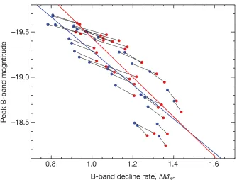
Effect of the metal content of the progenitor star population on the WLR. The models explore two extreme values of the metallicity: 3 times (red points) and 0.3 times the solar value (blue points). For clarity, each model has been averaged over all viewing angles, and black lines connect similar explosion models of differing metallicity. The coloured lines are linear fits to the WLR of the two metallicity samples separately. The diversity introduced by metallicity variations follows the general width–luminosity trend, but the slightly different normalization and slope of the relation for different metallicity samples indicates a potential source of systematic error in distance determinations.

NATURE

|

Vol 460

|

13 August 2009

LETTERS

871

Figure 1.5 Effect of progenitor metallicity on the width-luminosity relation, reproduced from Kasen et al. (2009). The red points are SN Ia progenitor models with a metallicity

of 3 times the solar value (3Z), while the blue points are models with 0.3 times the solar

metallicity (0.3Z). The metallicity variations are in the general direction of the

width-luminosity relation; however, their effect is not completely corrected for by the relation.

on average, which can be qualitatively explained by the Timmes et al. (2003) result. Using

a sample of 168 nearby SNe Ia, Neill et al. (2009) followed up on the work of Howell et al.

(2009) and obtained matched-aperture host galaxy photometry from theGalaxy Evolution

Explorer(GALEX), SDSS, and the Third Reference Catalogue of Bright Galaxies (RC3).

They found that the relation between inferred metallicity and56Ni mass for local hosts

agrees with the Howell et al. (2009) trend at higher redshifts, but is also consistent with

no trend. In addition, after imposing cuts to obtain a low-stretch, low-extinction sample

of hosts, they found a 2.1σ correlation between HR and luminosity-weighted age such

that SNe Ia in older hosts appear brighter after correcting for stretch and color. However,

this sample contained only 22 hosts and when the full sample was used, they found no

such correlation.

(33)

Kelly et al. (2010) used_∼60 nearby SNe Ia in the redshift range 0.015<z<0.08 and

computed stellar masses of the host galaxies from SDSS photometry. They analyzed their

SN sample using two versions of MLCS and two versions of SALT and found the same

result: SNe Ia occuring in massive hosts are_∼10% brighter after light curve correction.

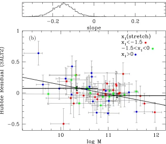
In fact, fitting for a linear relationship between HR (defined as µSN−µz) and host mass

yielded a_∼3σ significance of a non-zero slope. This is shown for the case of SALT2

HRs in Figure 1.6. If the higher-mass galaxies in this sample also have higher

metal-licities (following the mass-metallicity relation), this trend agrees with the Gallagher et

al. (2008) trend of HR with metallicity and also the theoretical work of Timmes et al.

(2003) and Kasen et al. (2009). Kelly et al. (2010) points out the troubling fact that

cor-relations between HR and progenitor properties can potentially bias SN Ia cosmological

measurements, since progenitors of SNe at high redshift are likely to be younger and more

metal-poor than their counterparts at low redshift. The relatively high statistical

signifi-cance of this discovery by Kelly et al. (2010) and its implications for cosmology spurred

other SN teams to further investigate correlations between HR and host properties in their

SN samples.

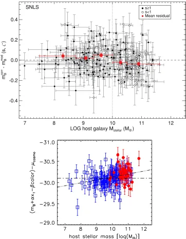
Sullivan et al. (2010) searched for host-galaxy dependencies using the three-year

SNLS sample and the SiFTO light-curve fitter (Conley et al. 2008), which is similar

to SALT2 and parameterizes the light curve by stretch (s) and color (_C). Using stellar

population synthesis models and optical photometry they derived host galaxy properties

such as stellar mass and recent star formation per unit mass (known as specific star

for-mation, sSFR). For the SNLS data atz_≤0.85 they found that SNe Ia in low-sSFR host

galaxies, and SNe Ia in massive host galaxies, are systematically brighter by 0.06₋0.09

mag (with significances>3σ) after correcting for SN stretch and color. Assuming host

mass is a proxy for host metallicity and thus metallicity of the progenitor, these results

indicate that metal-rich environments host brighter SNe after light-curve correction. This

agrees with the previously published trends described above, and their results are also

consistent with the progenitor metallicity-luminosity relation of Timmes et al. (2003) and

Understanding Type Ia Supernovae Through Their Host Galaxies Using the SDSS-II Supernova Survey

University of Pennsylvania

ScholarlyCommons

Understanding Type Ia Supernovae Through Their

Host Galaxies Using the SDSS-II Supernova

Survey

Ravi Ryan Gupta

Understanding Type Ia Supernovae Through Their Host Galaxies Using

the SDSS-II Supernova Survey

Dedication

For Mom and Pop, who made many sacrifices to open as many doors for

me as possible, and who encouraged me to pursue my interests, whatever

they may be. From them I learned the importance of education, working

hard, and trying my best, no matter what. And for my girlfriend, Kelly,

who has been a constant source of support, care, and love despite being

3810.4 kilometers away.

Acknowledgments

Contents

List of Tables

List of Figures

Chapter 1

Introduction

1.1

Cosmology and the Expanding Universe

1.1.1

Expansion History

1.1.2

Magnitudes and Distance Moduli

1.1.3

A Census of the Universe

1.2

Type Ia Supernovae

1.2.1

Classification and Progenitors

1.2.2

Standardizable Candles

1.2.3

Evidence for Acceleration

Z

1.3

Supernovae in the Sloan Digital Sky Survey

1.4

Type Ia Supernova–Host Galaxy Correlations

1.4.1

Environmental Dependencies on SN Luminosities

1.4.2

Correlations with Hubble Residuals

indications that type Ia supernovae are nearly standard (as opposed to

merely standardizable) candles in the near-infrared

.

Without introducing any artificial tuning, the luminosity of the

models correlates with the light-curve decline rate, giving a width–

luminosity relation (WLR) similar to that observed (Fig. 3). A

cor-relation is also found between brightness and the colour measured at

peak. The r.m.s. scatter in the model WLR alone is 24%, while using

both decline rate and colour reduces the dispersion to 21%—similar

to, but slightly greater than, the

,

16% that is observed

. The larger

diversity seen in the models suggests that additional important

physics may constrain the ignition and detonation conditions to a

range narrower than that considered here. As in observations, the

calibration of the models can be improved by using additional

information from the light curve. For example, including the shape

of the light curve in several optical and near-infrared wavelength

bands reduces the scatter to only 15%.

For a given mass of

Ni, the residual scatter in the model WLR

reflects individual features of the supernova debris structure. The

turbulent deflagration phase imprints density and chemical

inhomo-geneities, which lead to variations in the timescale for photons to

diffuse out of the debris. In addition, the global asymmetry—due to

asymmetric ignition conditions or off-centre detonation points—

gives rise to anisotropic emission, so that the brightness and duration

of most models vary by 20–30%, depending of the angle from which

they are viewed. Although the adoption of a two-dimensional

geo-metry may exaggerate global asymmetries, spectropolarization

observations reveal that type Ia supernovae typically possess

aspheri-city near or just below the level predicted here

_.

_{. The larger}

_{. Dimmer supernovae}

_{and observational}

_{that the metallicity of the white dwarf will affect the}

_{Ni yield at}